Normal Mode Analysis for Connected Plate Structure Using Efficient Mode Polynomials with Component Mode Synthesis

Abstract

In the engine room and stern adjacent to the main excitation force of the ship, there are many fuel and fresh water tank structures required for ship operation which are always exposed to vibrations. Therefore, it is necessary to review the anti-vibration design to prevent such vibration problems at the design stage, and for this reason, although commercial finite element analysis (FEA) programs are widely used, approximate analysis methods are still developed and used because of the limited time until modeling and analysis results are obtained. Until now, only known elastic boundary conditions have been used in many studies using approximate analysis methods used to calculate natural vibrations for beams or plates. However, many local structures, such as tank edges and equipment foundations, consist of connected structures and it is very difficult to find suitable elastic boundary conditions. Vibration analysis of many local structures in ships, such as tanks and supports for equipment, can be simplified by breaking them up into smaller subsystems which are related through geometrical conditions and natural conditions at junctions. In this study, polynomials for simple support and fixed support were proposed to represent each subsystem and a polynomial to be applied to the plate constituting the tank was proposed by combining them. Until now, there have been many studies on single beams or single plates for approximate analysis. However, there was no research on this to the extent that no reference material could be found for the connected structure. The proposed method has been applied to tanks which are bounded by bulkhead and a deck. The results of this study shows good agreements with those obtained by the FEA Software (Patran/Nastran).

1. Introduction

In the engine room and stern adjacent to the main excitation force of the ship, there are many fuel and fresh water tank structures required for ship operation which are always exposed to vibration. If a vibration problem occurs after construction or delivery, there is a large loss in terms of ship quality, such as reinforcement cost and delivery delay. Therefore, it is necessary to review the anti-vibration design to prevent such vibration problems in the design stage, and for this reason, each shipyard has developed and used an approximate vibration calculation program according to the circumstances of the design.

In the case of this approximate analytical calculation method, the Bernoulli–Euler beam theory [1] is mainly used as a mode function. Since the computational process is complicated, many studies using polynomials with beam properties have been conducted to simplify it.

Han [2,3] defined the assumed mode function by combining the Euler beam mode function with the same boundary condition and performed vibration analysis for the plate.

Kim [4] performed normal mode analysis in consideration of the effects of rotational inertia and shear deformation of plates and beams using a polynomial with Timoshenko’s beam properties.

Chung [5] considered the rotational elastic constraints at both ends of the structure in order to provide an appropriate boundary condition.

In recent studies, mode functions are defined using Euler beams [6], Legendre polynomials [7] and orthogonality [8] and are applied not only to calculation of natural frequencies but also to calculations of hull deformation when a ship is impacted by waves while in operation.

In addition, a study on the method of searching for the crack point of a beam using the Euler beam theory [9] was also carried out and vibration analysis of a wedge beam was carried out [10]. Many studies such as this are being conducted using the characteristics of Euler beams.

For vibration analysis of the connection structure, it is important to define the function of each member and the constraint conditions of the connection part. Many researchers, such as Hurty, defined and used the equation using Euler beam characteristics for the dynamic analysis of aircraft wings [11,12].

For vibration analysis, such as panel structure, a method of deriving a polynomial with Timoshenko’s beam property is presented. Furthermore, Bhat [13] uses a polynomial as mode functions. However, all of the above studies are used given elastic boundary conditions and no studies on deriving appropriate boundary conditions have been found. This is the biggest reason why there has been no study of normal mode analysis using the assumed mode function over the past 10 years.

Many local structures, such as tank edges and equipment foundations, consist of connected structures, and there is a need to find the suitable elastic boundary condition to find the normal mode frequencies.

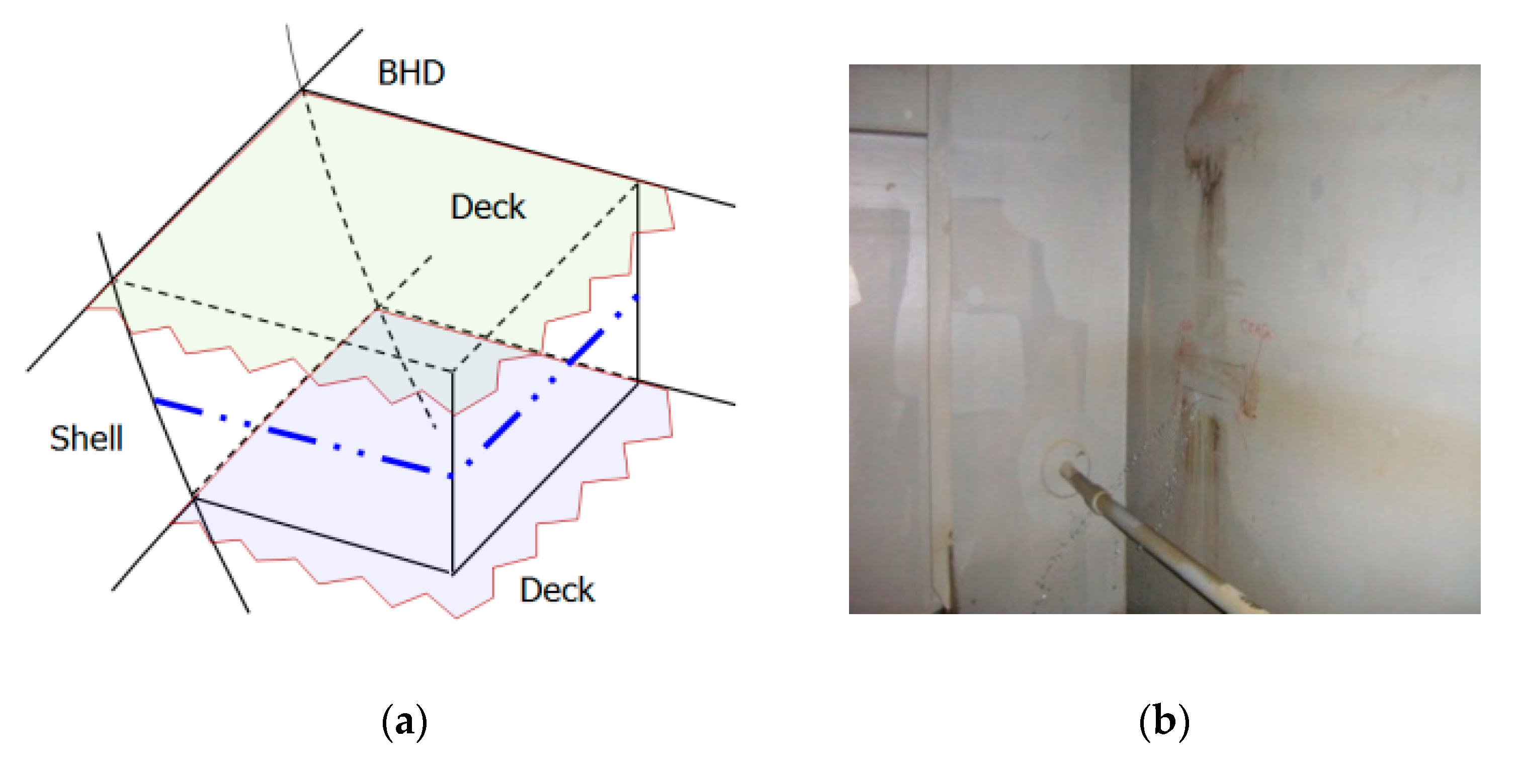
Vibration analysis of many local structures in ships as Figure 1, such as tanks and supports for equipment, can be simplified by breaking them up into smaller subsystems which are related through geometrical conditions and natural conditions at junctions [14,15]. We have established a method to calculate the actual boundary condition at the junction of the connection structure at the tank wall.

To do this, firstly, we formalize the polynomials for simple support and fixed support that were proposed to represent each subsystem, and in order to verify the validity of the polynomials, we performed the normal mode calculation using component mode synthesis. The purpose of this study was to propose a method of satisfying the actual boundary condition by combining the mode function including the simple support and the fixed support boundary condition in the plate structure.

For the finite element analysis (FEA) result and the calculation result, the error was confirmed by performing calculations while changing the thickness of the plate to 20T, 15T and 25T.

Among the reference literature, the properties of the structure of the tank manufactured for the experimental method [16] were applied to the method suggested in this study and the results were compared with the experimental results.

When the FEA results and calculation deviations are confirmed, it is considered to be very useful as a methodology that can be applied to the natural frequency calculation of the connected plate structure proposed in this study.

2. Definition of Assumed Mode Functions

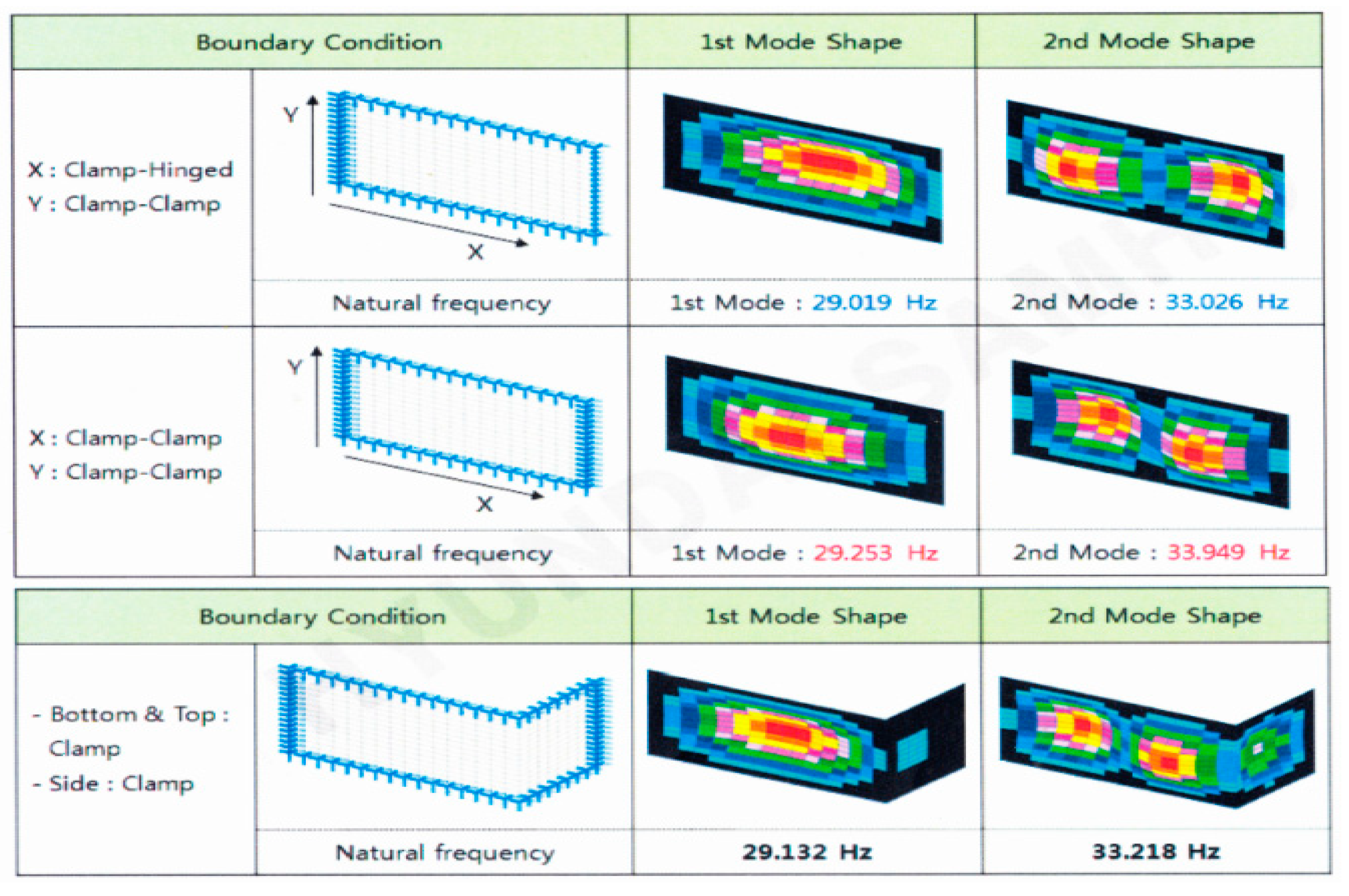
In Figure 2, the natural frequencies and natural modes of the single plate and the connecting plate structures were confirmed through the finite element analysis (FEA) program. As a result, it can be confirmed that the first and second natural modes of the main structure among the connected plate structures are similar to the analysis results of the single plate, and the natural frequency is in the middle of the fixed-simple support and fixed-fixed support conditions of the single plate. Therefore, the mode function of the combined state of the two conditions was defined and the result was confirmed.

First, as a method to effectively assume the plate structure, a method of assuming a linear combination of simple beam mode functions in the x-axis and y-axis directions is commonly used. In other words,

$$w\left(x,y,t\right)={\displaystyle \sum }_{m=1}^p{\displaystyle \sum }_{n=1}^q{A}_{mn}\left(t\right)\cdot X_m\left(x\right)\cdot Y_n(y)$$

(1)

where X_m(x), Y_n(y) are the mode functions of the beam in the x-axis and y-axis directions, p and q are the terms of the mode function and A_mn(t) is the unknown coefficient for each term.

Among the assumed mode functions of a beam, the polynomial of the first-order mode function that satisfies the fixed-fixed boundary condition (Ψ), the fixed-simple boundary condition (Φ) and the simple-fixed boundary condition (γ) is Equations (2)–(4) and it can be obtained respectively.

$${\psi }_1\left(\eta \right)=A_1{(\eta +1)}^2{(\eta -1)}^2\hspace{1em}-1\le \eta \le 1$$

(2)

$${\phi }_1\left(\eta \right)=B_1\left({\eta }^4-{\eta }^3-3{\eta }^2+\eta +2\right)$$

(3)

$${\gamma }_1\left(\eta \right)=C_1\left({\eta }^4+{\eta }^3-3{\eta }^2-\eta +2\right)$$

(4)

The coefficients A₁, B₁ and C₁ are implemented using the orthogonal formula of the beam function.

$${{\displaystyle \int }}_{-1}^1{\psi }_i{\psi }_{j}d\eta ={\delta }_{ij}$$

(5)

$${{\displaystyle \int }}_{-1}^1{\phi }_i{\phi }_{j}d\eta ={\delta }_{ij}$$

(6)

$${{\displaystyle \int }}_{-1}^1{\gamma }_i{\gamma }_{j}d\eta ={\delta }_{ij}$$

(7)

where i, j is the vibration order and δ_ij is Kronecker delta.

$$A_1=\frac{{{\displaystyle \int }}_{-1}^1{\psi }_1^{2}d\eta }{\sqrt{{{\displaystyle \int }}_{-1}^1{({\eta }^4-2{\eta }^2+1)}^{2}d\eta }}$$

(8)

$$B_1=\frac{{{\displaystyle \int }}_{-1}^1{\phi }_1^{2}d\eta }{\sqrt{{{\displaystyle \int }}_{-1}^1{({\eta }^4-{\eta }^3-3{\eta }^2+\eta +2)}^{2}d\eta }}$$

(9)

$$C_1=\frac{{{\displaystyle \int }}_{-1}^1{\gamma }_1^{2}d\eta }{\sqrt{{{\displaystyle \int }}_{-1}^1{({\eta }^4+{\eta }^3-3{\eta }^2-\eta +2)}^{2}d\eta }}$$

(10)

The waveform function of the second mode or more can be implemented from the following Equations (11)–(13).

$${\psi }_k=A_k\left[{\psi }_{k-1}\cdot \eta -{\displaystyle \sum }_{i=1}^{k-1}{a}_{ki}\cdot {\psi }_{k-1}\right]$$

(11)

$${\phi }_k=B_k\left[{\phi }_{k-1}\cdot \eta -{\displaystyle \sum }_{i=1}^{k-1}{b}_{ki}\cdot {\phi }_{k-1}\right]$$

(12)

$${\gamma }_k=B_k\left[{\gamma }_{k-1}\cdot \eta -{\displaystyle \sum }_{i=1}^{k-1}{c}_{ki}\cdot {\gamma }_{k-1}\right]$$

(13)

The coefficients a_ki, b_ki, c_ki can be obtained from the orthogonal relation of the complementary function and the Equations (11)–(13) above.

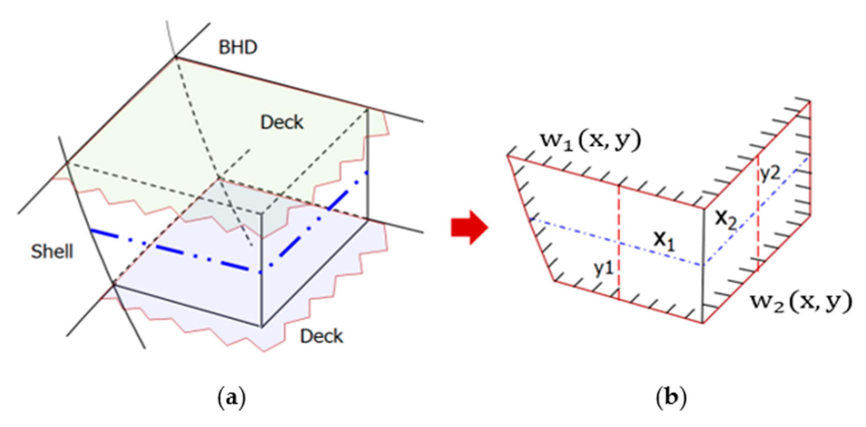
In Figure 3, the y-axis of the w₁(x, y) plate is constrained by the structure between the deck and the deck, so the mode function is assumed only in the fixed-fixed support condition, and in the case of the x-axis, the fixed-fixed ($\psi$) and fixed-simple ($\varphi$) mode functions are expressed as a combination.

The case of w₂(x, y) was also defined in a similar way to the above, but the mode function of the x-axis was summarized using a simple-fixed ($\varphi$) support assume mode function.

$$x_1\left(\eta \right)={\displaystyle \sum }_{i=1}^m\left({\psi }_i\left(\eta \right)p_{Ai}\left(t\right)+{\varphi }_i\left(\eta \right)q_{Ai}\left(t\right)\right)$$

(14)

$$y_1\left(\eta \right)={\displaystyle \sum }_{j=1}^n\left({\psi }_j\left(\eta \right)p_{Bj}\left(t\right)\right)$$

(15)

$$w_1\left(x,y\right)=f_{A11}{\psi }_1{\psi }_1+\cdots +f_{Amn}{\psi }_m{\psi }_n+g_{A11}{\varphi }_1{\psi }_1+\cdots +g_{Amn}{\varphi }_m{\psi }_n$$

(16)

$$x_2\left(\eta \right)={\displaystyle \sum }_{k=1}^s\left({\psi }_k\left(\eta \right)p_{\mathrm{ck}}\left(t\right)+{\gamma }_k\left(\eta \right)q_{ck}\left(t\right)\right)$$

(17)

$$y_2\left(\eta \right)={\displaystyle \sum }_{l=1}^u\left({\psi }_l\left(\eta \right)p_{Dl}\left(t\right)\right)$$

(18)

$$w_2\left(x,y\right)=f_{B11}{\psi }_1{\psi }_1+\cdots +f_{Bsu}{\psi }_s{\psi }_u+g_{B11}{\gamma }_1{\psi }_1+\cdots +g_{Bsu}{\gamma }_s{\psi }_u$$

(19)

where $p_{Ai}\left(t\right),q_{Ai}\left(t\right),p_{Bj}\left(t\right),p_{Ck}\left(t\right),q_{Ck}\left(t\right),p_{Dl}\left(t\right)$ are the general coordinate system in the assumed mode function of beam and $f_{A11}\left(t\right),\cdots ,f_{Amn}\left(t\right),g_{A11}\left(t\right),\cdots ,g_{Amn}\left(t\right),f_{B11}\left(t\right),\cdots ,f_{Bsu}\left(t\right),g_{B11}\left(t\right),\cdots ,g_{Bsu}\left(t\right)$ are the general coordinate system of the assumed mode function that makes up the wall structure.

3. Component Mode Synthesis

Figure 4 shows the general tank structure shape inside the hull. For the analysis of the connected structure, the component mode synthesis method [14,15] that satisfies the boundary condition at the structure connection was used.

The connection structure, as shown in Figure 4, must satisfy the continuous conditions for the angle and moment as follows.

[Slope Continuity]

$$\frac{\partial w_1}{\partial x}\left(1,\mathrm{y}\right)-\frac{\partial w_2}{\partial x}\left(-1,y\right)=0$$

(20)

$$\frac{1}{l_1}\left[g_{A11}{{\varphi }^{\prime }}_1{\psi }_1+\cdots +g_{Amn}{{\varphi }^{\prime }}_m{\psi }_n\right]-\frac{1}{l_3}\left[g_{B11}{{\gamma }^{\prime }}_1{\psi }_1+\cdots +g_{Bsu}{{\gamma }^{\prime }}_s{\psi }_u\right]=0$$

(21)

$$g_{Bsu}=\frac{1}{\alpha }\left[g_{A11}·\frac{{{\varphi }^{\prime }}_1{\psi }_1}{{{\gamma }^{\prime }}_s{\psi }_u}+\cdots +g_{Amn}·\frac{{{\varphi }^{\prime }}_m{\psi }_n}{{{\gamma }^{\prime }}_s{\psi }_u}\right]-\left[g_{B11}·\frac{{{\gamma }^{\prime }}_1{\psi }_1}{{{\gamma }^{\prime }}_s{\psi }_u}+\cdots +g_{Bsu-1}·\frac{{{\gamma }^{\prime }}_s{\psi }_{u-1}}{{{\gamma }^{\prime }}_s{\psi }_u}\right]$$

(22)

[Moment Continuity]

$$\frac{{\partial }^2{w}_1}{\partial x^2}\left(1,\mathrm{y}\right)+\frac{{\partial }^2{w}_2}{\partial x^2}\left(-1,y\right)=0$$

(23)

$$f_{Bsu}=-\frac{1}{{\alpha }^2}\left[f_{A11}·\frac{\psi {″}_1{\psi }_1}{\psi {″}_s{\psi }_u}+\cdots +f_{Amn}·\frac{\psi {″}_m{\psi }_n}{\psi {″}_s{\psi }_u}\right]-\left[f_{B11}·\frac{\psi {″}_1{\psi }_1}{\psi {″}_s{\psi }_u}+\cdots +f_{Bsu-1}·\frac{\psi {″}_s{\psi }_{u-1}}{\psi {″}_s{\psi }_u}\right]$$

(24)

As shown in the above equation, only the degree of freedom (DOF) that satisfies the simple support boundary condition is involved for the slope, and when the moment boundary condition is satisfied, only the fixed DOF is involved.

4. Normal Mode Analysis of Connected Structure

For vibration analysis by the classical approximate solution using the assumed mode function, the elastic energy and kinetic energy equations of the analysis target system are required. As for the waveform assumption function, Euler’s beam function or Timoshenko’s beam function, taking into account the shear deformation effect, are generally used, and the vibration analysis method using the Timoshenko beam function has already been formulated by Kim [4] or Chung [5].

In this study, in order to confirm the usefulness of the vibration analysis formulation method for the connected structure, a polynomial with Euler’s beam property was first defined as an assumed mode function and the natural frequency of the connected plate was calculated.

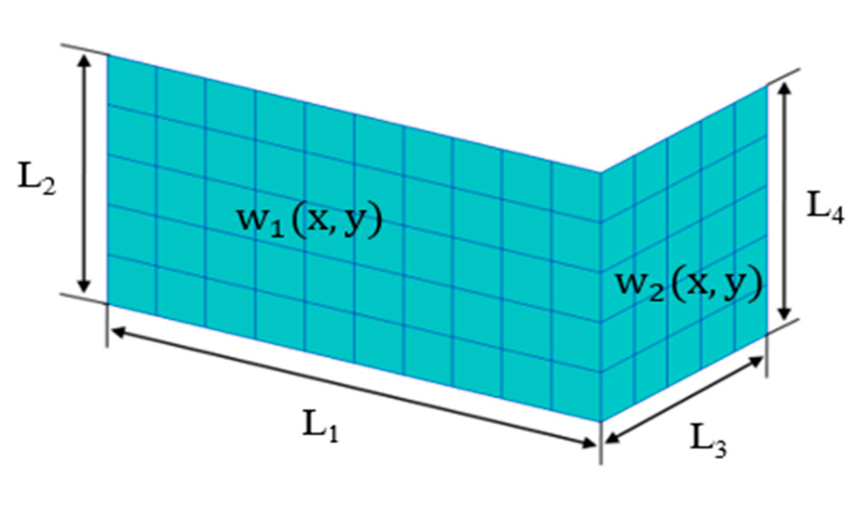
In Figure 4, the result of formulation calculation according to the change in $w_2\left(x,y\right)$ plate length in the connected structure was compared/reviewed with the results of the finite element analysis method (FEA). As shown in Figure 3, considering that the boundary of the tank structure is constrained by the deck and bulkheads, all corners were considered as fixed conditions.

Table 1. The property of model.

Thickness (mm)	Elastic Modulus (N/m2)	Density (kg/m3)
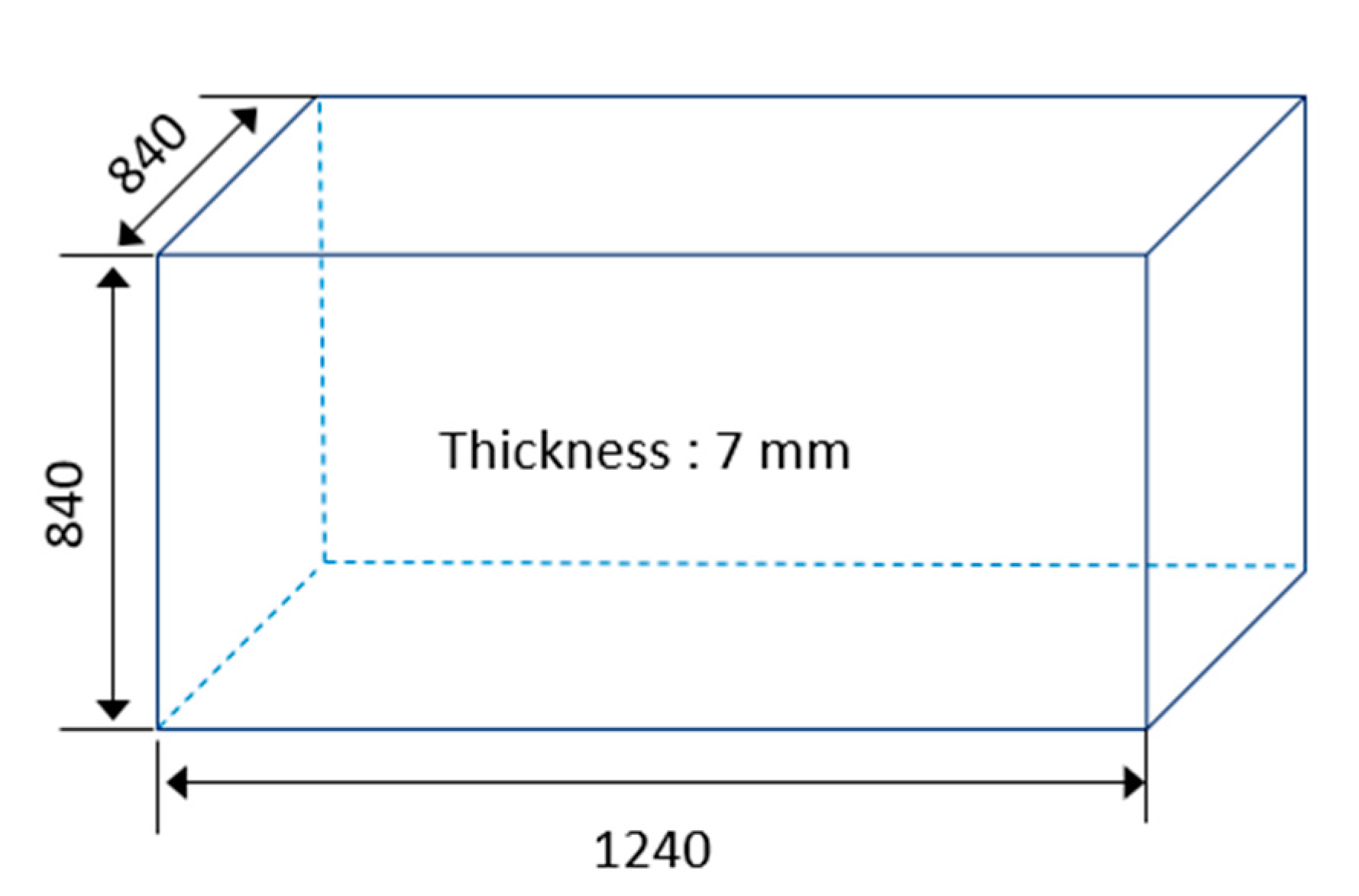
20.0	2.1 × 1011	7850

shows the properties of the structure expressed in Figure 4.

Table 2. The comparison of results (unit: Hz).

L1	L2	L3	L4	Calculation Results				FEA
				W1 Plate		W2 Plate		W1 Plate		W2 Plate
				1st	2nd	1st	2nd	1st	2nd	1st	2nd
10 m	2 m	2 m	2 m	28.258	29.172	39.6509	79.560	28.119	29.150	38.911	78.265
10 m	2 m	4 m	2 m	28.258	29.171	30.1476	38.2295	28.117	29.132	30.067	37.318
10 m	2 m	6 m	2 m	28.258	29.1707	28.8382	31.7294	28.116	29.161	28.752	31.631
10 m	2 m	8 m	2 m	28.258	29.1706	28.4347	29.9250	28.114	29.141	28.323	29.910
L1	L2	L3	L4	Calculation Results				FEA
				W1 Plate		W2 Plate		W1 Plate		W2 Plate
				1st	2nd	1st	2nd	1st	2nd	1st	2nd
10 m	4 m	2 m	4 m	7.3174	8.4221	24.2613	66.5475	7.299	8.4139	22.595	65.952
10 m	4 m	4 m	4 m	7.3174	8.4211	9.9257	20.4227	7.2926	8.3736	9.9945	20.678
10 m	4 m	6 m	4 m	7.3174	8.4209	8.0618	11.9233	7.2894	8.4561	8.06	12.036
10 m	4 m	8 m	4 m	7.3174	8.4207	7.5330	9.4307	7.2854	8.3852	7.5275	9.4263
L1	L2	L3	L4	Calculation Results				FEA
				W1 Plate		W2 Plate		W1 Plate		W2 Plate
				1st	2nd	1st	2nd	1st	2nd	1st	2nd
10 m	5 m	2 m	5 m	4.8210	6.0355	22.7025	65.2687	4.8372	6.1126	21.289	64.061
10 m	5 m	4 m	5 m	4.8210	6.0346	7.7592	18.7341	4.8271	6.0555	7.9146	19.248
10 m	5 m	6 m	5 m	4.8210	6.0343	5.6593	9.8768	4.8218	6.1803	5.7169	10.156
10 m	5 m	8 m	5 m	4.8206	6.0342	5.0606	7.1596	4.8151	6.0707	5.105	7.2607
L1	L2	L3	L4	Calculation Results				FEA
				W1 Plate		W2 Plate		W1 Plate		W2 Plate
				1st	2nd	1st	2nd	1st	2nd	1st	2nd
10 m	6 m	2 m	6 m	3.4765	4.7952	21.9302	64.6035	3.5219	4.9357	20.579	63.508
10 m	6 m	4 m	6 m	3.4764	4.7944	6.6836	17.8992	3.5076	4.8633	6.8827	18.545
10 m	6 m	6 m	6 m	3.4764	4.7942	4.4059	8.8678	3.4994	5.0291	4.5036	9.2425
10 m	6 m	8 m	6 m	3.4764	4.7940	3.7410	6.0089	3.451	3.559	4.715	5.081
L1	L2	L3	L4	Calculation Results				FEA
				W1 Plate		W2 Plate		W1 Plate		W2 Plate
				1st	2nd	1st	2nd	1st	2nd	1st	2nd
10 m	8 m	2 m	8 m	2.166	3.6533	19.9793	63.9653	2.1509	3.7996	19.815	62.33
10 m	8 m	4 m	8 m	2.1658	3.6527	5.7362	16.6369	2.2379	3.7774	5.9676	17.907
10 m	8 m	6 m	8 m	2.1658	3.6525	3.2489	7.9454	2.2234	4.0017	3.3912	8.4389
10 m	8 m	8 m	8 m	2.1658	3.6525	2.4780	4.9726	2.206	3.8013	2.6315	5.2166
L1	L2	L3	L4	Calculation Results				FEA
				W1 Plate		W2 Plate		W1 Plate		W2 Plate
				1st	2nd	1st	2nd	1st	2nd	1st	2nd
10 m	10 m	2 m	10 m	1.5860	3.1835	19.6919	63.6776	1.6688	3.438	19.569	61.910
10 m	10 m	4 m	10 m	1.5858	3.1830	5.3571	16.8109	1.6906	3.3351	5.5970	17.634
10 m	10 m	6 m	10 m	1.5858	3.1829	2.7747	7.6042	1.6697	3.6048	2.9365	8.112
10 m	10 m	8 m	10 m	1.5858	3.1829	1.9366	4.5556	1.6448	3.3624	2.1369	4.8292

shows the calculation results according to the length ratio of the connection structure compared with the FEA results.

Table 3. FEA Result of single plate for simply supported boundary conditions (unit: Hz).

Single Plate for Simply Supported Boundary Conditions
L1	L2	L3	L4	W1 Plate		W2 Plate
				1st	2nd	1st	2nd
10 m	6 m	2 m	6 m	3.4648	4.7624	20.477	63.273
10 m	6 m	4 m	6 m	3.4648	4.7624	6.6272	17.055
10 m	6 m	6 m	6 m	3.4648	4.7624	4.3862	8.7119
10 m	6 m	8 m	6 m	3.4648	4.7624	3.7278	5.9475

shows the finite element analysis results for the fixed-simple support condition for one plate for the case where L1:L2 is 1:0.6 among the calculation results of Table 2.

Compared with the calculation results in Table 2, it shows the lowest overall value. This is the part where it is judged that the fixed support condition as well as the simple support condition affects the connection part. Looking at the calculation results of the formalization method according to the length change in Table 2, the first mode is similar to the finite element analysis result, but in the second mode, the ratio of length (L₁, L₃): height (L₂, L₄) should be less than 1:0.6. In the case of the finite element analysis, the result is less than 5%, and when the length: height ratio is 1:1, there is a difference of about 10%, but the actual tank structure of the ship has a length: height ratio that is usually less than 1:0.5.

Generally, a 10% margin is usually considered in the FEA result for examining the resonance of the wall in the initial design stage and shows that it is similar to the FEA result in the low frequency region of interest in the shipyard.

In addition, it was confirmed that the plate thickness was similar to the FEA result by performing calculations for the cases of 15T and 25T. And each property value is shown in

Table 4. The property of model.

Thickness (mm)	Elastic Modulus (N/m2)	Density (kg/m3)
15.0	2.1 × 1011	7850

and

Table 5. The property of model.

Thickness (mm)	Elastic modulus (N/m2)	Density) kg/m3)
25.0	2.1 × 1011	7850

, and the results are shown in

Table 6. The comparison of results (unit: Hz).

L1	L2	L3	L4	Calculation Results				FEA
				W1 Plate		W2 Plate		W1 Plate		W2 Plate
				1st	2nd	1st	2nd	1st	2nd	1st	2nd
10 m	2 m	2 m	2 m	21.194	21.878	29.739	62.391	21.089	21.752	29.334	62.651
10 m	2 m	4 m	2 m	21.194	21.878	22.599	28.245	21.088	21.743	22.468	28.025
10 m	2 m	6 m	2 m	21.194	21.878	21.628	23.753	21.087	21.759	21.513	23.574
10 m	2 m	8 m	2 m	21.194	21.878	21.326	22.406	21.086	21.747	21.22	22.288
L1	L2	L3	L4	Calculation Results				FEA
				W1 Plate		W2 Plate		W1 Plate		W2 Plate
				1st	2nd	1st	2nd	1st	2nd	1st	2nd
10 m	5 m	2 m	5 m	3.616	4.525	16.045	20.873	3.635	4.608	16.032	20.823
10 m	5 m	4 m	5 m	3.616	4.525	5.811	14.023	3.672	4.565	5.976	14.489
10 m	5 m	6 m	5 m	3.616	4.525	4.244	7.385	3.661	4.708	4.352	7.747
10 m	5 m	8 m	5 m	3.616	4.525	3.796	5.364	3.618	4.576	3.840	5.480
L1	L2	L3	L4	Calculation Results				FEA
				W1 Plate		W2 Plate		W1 Plate		W2 Plate
				1st	2nd	1st	2nd	1st	2nd	1st	2nd
10 m	10 m	2 m	10 m	1.190	2.580	14.770	15.757	1.293	2.587	14.746	15.789
10 m	10 m	4 m	10 m	1.190	2.580	5.218	13.338	1.270	2.507	5.127	13.238
10 m	10 m	6 m	10 m	1.190	2.580	2.081	3.455	1.255	2.683	3.455	3.535
10 m	10 m	8 m	10 m	1.190	2.580	1.453	2.913	1.236	2.528	1.606	2.963

and

Table 7. The comparison of results (unit: Hz).

L1	L2	L3	L4	Calculation Results				FEA
				W1 Plate		W2 Plate		W1 Plate		W2 Plate
				1st	2nd	1st	2nd	1st	2nd	1st	2nd
10 m	2 m	2 m	2 m	35.324	36.463	49.564	111.978	35.098	36.143	48.594	112.54
10 m	2 m	4 m	2 m	35.324	36.463	37.665	47.076	35.096	36.128	37.314	46.421
10 m	2 m	6 m	2 m	35.324	36.463	36.047	39.559	35.095	36.153	35.77	39.093
10 m	2 m	8 m	2 m	35.324	36.463	35.324	37.344	35.094	36.134	35.305	37.003
L1	L2	L3	L4	Calculation Results				FEA
				W1 Plate		W2 Plate		W1 Plate		W2 Plate
				1st	2nd	1st	2nd	1st	2nd	1st	2nd
10 m	5 m	2 m	5 m	6.027	7.542	26.742	34.789	6.056	7.675	26.675	34.578
10 m	5 m	4 m	5 m	6.027	7.542	9.684	19.417	6.044	7.604	9.951	19.262
10 m	5 m	6 m	5 m	6.027	7.542	7.074	12.306	6.101	7.841	7.250	12.898
10 m	5 m	8 m	5 m	6.027	7.542	6.326	8.940	6.029	7.623	6.397	9.126
L1	L2	L3	L4	Calculation Results				FEA
				W1 Plate		W2 Plate		W1 Plate		W2 Plate
				1st	2nd	1st	2nd	1st	2nd	1st	2nd
10 m	10 m	2 m	10 m	1.983	4.300	24.617	26.261	2.155	4.314	24.600	26.275
10 m	10 m	4 m	10 m	1.983	4.300	8.700	22.230	2.117	4.480	8.541	22.045
10 m	10 m	6 m	10 m	1.983	4.300	3.469	5.759	2.091	4.470	3.679	5.889
10 m	10 m	8 m	10 m	1.983	4.300	2.421	4.854	2.050	4.460	2.677	4.936

. The shape of the tank is shown in Figure 4.

5. Comparison of Experimental Models

In open literature, there are cases in which experimental verification was conducted in the actual ship’s fresh water tank [17] or outdoor wall structures, such as swimming pools [18].

There are cases [19,20] in which a small experimental tank was manufactured and experimentally verified but it is difficult to accurately compare them because there is a difference from the actual model (reinforcement plate or opening plate).

Among the reference literature, there is a case of verifying the natural frequency through an impact test on a small rectangular tank as Figure 5 [8]. The properties of the plate were calculated by applying the method proposed in this study and the results are included in this content.

In

Table 8. The comparison results.

Order	Experiment	Calculated Result	Deviation (%)
1	61.3 Hz	64.3 Hz	+4.8
2	89.2 Hz	95.9 Hz	+7.5

, it can be seen that there is no significant difference in the calculation results, even when compared with the experimental results.

6. Conclusions

In order to satisfy the boundary condition of the connected structure, an efficient method of minimizing the increase in the degree of freedom is proposed by assuming the wave function as a combination of polynomials that satisfy the simple and fixed support conditions.

Additionally, its usefulness was verified by applying it to the flat plate connection structure.

In this study, a method of wave assumption function required for the analysis of natural vibrations of connecting beam structures, such as tanks and various auxiliary tables, which is limited in practicality due to the limitation of boundary condition settings, is presented.

In addition, it was confirmed that the validation of this study was within the deviation 10% by applying the model of the experimental method mentioned in the public literature.

References

1. Ahn, C.W.; Hong, D.K.; Kim, D.Y.; Choi, S.C.; Park, I.S. A Study on the Optimal Position Determination of Middle Supporting points to Maximize the First Natural Frequency of a Beam. Trans. Korean Soc. Noise Vib. Eng. 2001, 11, 89–95. [Google Scholar]
2. Han, S.Y. Vibration Analysis of Local Plate for the Hull Structure. Bull. Soc. Naval Archit. Korea 1994, 31, 33–35. [Google Scholar]
3. Han, S.Y.; Kweon, H. Development of the Program for Vibration Analysis of Local Plate with Appendage. In Proceedings of the Korean Society for Noise and Vibration Engineering Conference; Korean Society for Noise and Vibration Engineering: Seoul, Korea, 2000; pp. 311–321. [Google Scholar]
4. Kim, B.H.; Kim, J.H.; Cho, D.S. Free Vibration Analysis Stiffened Plates Using Polynomials Having the Property of Timoshenko Beam functions of the Korean Society for Noise and Vibration Engineering Conference; Korean Society for Noise and Vibration Engineering: Seoul, Korea, 2004; pp. 623–628. [Google Scholar]
5. Chung, J.H.; Chung, T.Y.; Kim, K.C. Vibration Analysis of Mindlin Plates Using Polynomials Having the Property of Timoshenko Beam Functions. J. Soc. Naval Archit. Korea 1992, 29, 158–172. [Google Scholar]
6. Ohashi, K. Numerical study of flows around a ship hull including elastic deformation effect using a mode function (2020). In Proceedings of the 6th European Conference on Computational Mechanics: Solids, Structures and Coupled Problems, ECCM 2018 and 7th European Conference on Computational Fluid Dynamics, ECFD, Glasgow, UK, 11–15 June 2018; pp. 2143–2152. [Google Scholar]
7. Hong, Y.; Kashiwagi, M.; Heo, K. Numerical calculations of wave-induced hydroelastic response of a ship with forward speed using legendre polynomials as mode functions. In Proceedings of the International Offshore and Polar Engineering Conference, Shanghai, China, 11–16 October 2020; pp. 3537–3543. [Google Scholar]
8. Masahiro, M. Methor for optimization of ship hull forms on wave analysis—Application of orthogonal mode function. Hitachi Zosen Tech. Rev. 1984, 45, 33–39. [Google Scholar]
9. Yoon, H.-I.; Son, I.-S.; Ahn, S.-J. Free Vibration Analysis of Euler-Bernoulli Beam with Double Cracks. J. Mech. Sci. Technol. 2007, 21, 476–485. [Google Scholar] [CrossRef]
10. Shin, Y.-J.; Yun, J.H. Vibration Analysis for the Euler-Bernoulli Wedge Beam by Using Differential Transformation Method. Trans. Korean Soc. Noise Vib. Eng. 2005, 15, 1318–1323. [Google Scholar]
11. Hurty, W.C. Vibrations of structural systems by component mode synthesis. J. Eng. Mech. Div. Proc. Am. Soc. Civil Eng. 1960, 86, 51–69. [Google Scholar]
12. Hurty, W.C. Dynamic analysis of structural systems using component modes. AIAA J. 1965, 3, 678–685. [Google Scholar] [CrossRef]
13. Bhat, R.B. Natural Frequencies of Rectangular Plates Using Characteristic Orthogonal Polynomials in Rayleigh-Ritz Method. J. Sound Vib. 1985, 102, 493–499. [Google Scholar] [CrossRef]
14. Thomson, W.T. Theory of Vibration with Applications, 4th ed.; Prentice Hall: Englewood Cliffs, NJ, USA, 1993; pp. 360–365. [Google Scholar]
15. Thorby, D. Structural Dynamics and Vibration in Practice, 1st ed.; Elsevier: London, UK, 2008; pp. 194–213. [Google Scholar]
16. Choi, S.-H.; Kim, K.-S.; Son, S.-W. Analytical and Experimental Study on Vibration Characteristics for Rectangular Tank Structure Filled with Fluid. Trans. Korean Soc. Noise Vib. Eng. 2002, 12, 195–203. [Google Scholar]
17. Seo, M.-K.; Seok, H.-I.; Lee, C.-W. Study on vibration Characteristics of Fluid Tank Structure for ship. Soc. Naval Arch. Korea 2013, 85–89. [Google Scholar]
18. Kwak, D.-H.; Kim, N.-S.; Kim, K.-S.; Rhee, W. Study on the Experimental of Pool Tank Filled Water and Damping Variation; Korean Society for Noise and Vibration Engineering: Seoul, Korea, 2012; pp. 768–769. [Google Scholar]
19. Kim, K.S.; Cho, H.D.; Kong, Y.M.; Heo, J.H. Experimental and Analytical Study on Hydroelastic Vibration of Tank; Korean Society for Noise and Vibration Engineering: Seoul, Korea, 2008; pp. 96–100. [Google Scholar]
20. Bae, S.-Y. A Study on Vibration Characteristics in Water Tank Structure. J. Soc. Naval Archit. Korea 2003, 40, 46–52. [Google Scholar]
Figure 1. Arrangement of fresh water and fuel tanks in ship: (a) the arrangement shape of the tank; (b) 1700 TEU Container fresh water tank wall damage.
Applsci 10 07717 g001
Figure 2. Finite element analysis (FEA) results of single and connected plates.
Applsci 10 07717 g002
Figure 3. The arrangement of the tank in a ship: (a) the general shape of tank; (b) simplification of the ship tank shape.
Applsci 10 07717 g003
Figure 4. The model for comparison of calculated results.
Applsci 10 07717 g004
Figure 5. The properties and shapes of experimental models.
Applsci 10 07717 g005