1. Introduction
Named entity recognition (NER) has received much attention in a wide range of natural language processing (NLP) tasks, such as question and answering, information extraction, and machine translation. NER techniques can be classified into four main streams: (1) a rule-based approach based on hand-crafted rules, (2) an unsupervised learning approach that relies on an algorithm without label data, (3) a feature-based supervised learning approach focused on a supervised learning algorithm with feature engineering, and (4) deep learning approaches that automatically detect the result from raw inputs [
1].
Recently, along with the development of a deep learning (DL) model, a neural network model has been successfully used for NER tasks. In general, the DL-based NER has used various input representations (e.g., word embedding, character-level, word-level) to learn how to encode a word and its context in input sequence and predict a word’s entity label. Most researchers have commonly employed bidirectional Long Short-Term Memory (LSTM) Conditional Random Field (CRF) as a basic DL architecture to encode contextual information and find the best label sequence:
Lample et al. [
2], used hierarchical bidirectional LSTM CRF set up with pre-trained word embedding and character-level LSTM-based word encoding.
Ma and Hovy [
3], also employed the bidirectional LSTM CRF but combined the character-level CNN-based word encoding with pre-trained word embedding to get the final result.
Rei et al. [
4] also used the bidirectional LSTM CRF but applied attention-based weighted sum, instead of concatenation, when combining character-level LSTM-based word encoding with the pre-trained word embedding.
Chiu and Nichols [
5] used the bidirectional LSTM and addition with Log-Sotfmax to get the output and employed word-level pattern-based word encoding and gazetteer-based word encoding in addition to the pre-trained word embedding and character-level Convolutional Neural Network (CNN)-based word encoding.
These works employed various input representations and combined all the representations at the embedding layer of their models (we call it early combination) and passed it through the main model block, bidirectional LSTM.
In contrast, Huang et al. [
6] delayed the combining position of some features’ encoding until the output of the bidirectional LSTM is ready. They passed only the pre-trained word embedding through the bidirectional LSTM and this output was combined with additional word encodings based on word spelling, contexts of word, Part-Of-Speech (POS) and chunk, and gazetteer. This delayed combination technique was used to avoid a potential feature collision, which may occur during passing the bidirectional LSTM block. However, they did not provide any comparison between delayed combination and early combination.
In this paper, we adapt the delayed combination approach and analyze its effectiveness by comparing it to the existing, commonly used, early combination approach, inspired by Huang et al., 2016. We adapt character-level CNN or LSTM-based word encoding and recent contextualized word embedding and designed CNN-based sentence encoding using a named entity dictionary as supplementary feature encodings, in addition to the common pre-trained word embedding. We pass the pre-trained word embedding and the contextualized word embedding through the separate bidirectional LSTM blocks, respectively, and then we combine the outputs with the CNN or LSTM-based word encoding and the CNN-based sentence encoding. This combined encoding is finally fed into the CRF to find the best named entity label sequence.
We compare the delayed combination model with the early combination model by evaluating our own implementation of the two approaches and also compare our result to the previous works having similar model architecture and features to show the effectiveness of the delayed combination model. The main differences between the two models are as follows:
The early combination model concatenates representations at the embedding layer and then passes them through the bidirectional LSTM CRF. During passing through the bidirectional LSTM blocks, some useful but less-dominant encoded information may be mixed and collide with others and, as a result, fail to be propagated to the output layer.
The delayed combination model is designed to preserve some feature representations until the last layer by bypassing the bidirectional LSTM blocks, considering the characteristics of each feature (more details are given in
Section 3). The comparison result shows that the delayed combination is able to boost the performance of the model.
The rest of the paper is organized as follows. Related works are described in
Section 2. We present the proposed model architecture in
Section 3. The experimental setup is shown in
Section 4. The results are presented and discussed in
Section 5. Finally, we conclude in
Section 6.
2. Related Work
Recently, deep learning has become a dominant model to achieve the state-of-the-art results in NER task. The crucial advantage is its ability to undertake representation learning. Most deep learning-based NER approaches have designed and utilized various features to encode input sequence, such as (1) pre-trained word embedding, (2) contextual word embedding, (3) character-level CNN or LSTM-based word encoding, (4) word-level pattern-based encoding, and (5) dictionary-based word encoding. These representations were combined and passed through the bidirectional LSTM CRF network to learn further contextual information. In this section, we explore various representations used for encoding the input sequence and how to combine and feed them into the network.
2.1. Distributed Representations for Input
The concept of distributed representations refers to the representation of a word or a sentence by mapping it to a numerical vector. The vector is used to capture the semantic and grammatical properties of words. We review the following four types of distributed representations that have been popularly used in the previous works.
2.1.1. Pre-Trained Word Embedding
Pre-trained word embedding is the main element for most NLP tasks, including NER. Typically, embedding is trained over a large corpus, such as Wikipedia, Common Crawl, or the Reuters RCV-1 corpus. In this section, we describe different algorithms for computing word representations.
Word2vec: Word2vec can be implemented in two methods: a continuous bag of words (CBOW) and a Skip-gram method [
7,
8,
9,
10,
11,
12]. Both are log-linear models that are very useful for discovering the degree of word similarity [
13]. In particular, CBOW provides slightly better accuracy for frequent words, whereas Skip-gram represents rare words well.
GloVe: GloVe was developed at Stanford [
14]. This process begins by going through the text in a corpus, after which it counts the occurrences of word couples that are close to each other in a given window size. The information is stored in a matrix called an occurrence matrix. This matrix is used to build word embedding by minimizing the cosine distance between words to ensure a high co-occurrence probability [
15].
FastText: FastText [
16] was made available by Facebook. This model suggests an NLP improvement over the Skip-gram model, which learns by n-gram embedding. The rationale behind this approach relies on the morphology and information encoding in a subword. This information can be used to generate an unseen and rare word [
17].
2.1.2. Contextual Embedding
One limitation of the pre-trained word embeddings is that a word is represented by a unique single embedding regardless of its context. However, it is very common that a word could have a different meaning in a different context. For example, each ‘bank’ has a different meaning in ‘bank account’ and ‘river bank’. To avoid fixed embedding for each word, several studies have proposed contextual word representation techniques such as ELMO and BERT. ELMO [
18] is a character-based model, while BERT takes input as subwords and learns embeddings from the subwords. BERT has inspired many recent NLP research and language models, for instance XLNet [
19], RoBERTa [
20], and DistilBERT [
21].
2.1.3. Word-Level and Character-Level Representations
The pre-trained word embeddings and contextual embeddings learn the representations from the context of a word in a sentence, but does not consider and learn the character composition of a word, which are very important especially in the NER task because we often can infer the named entity (NE) type of a word from its character composition. To make up for this weak point, two different word representation techniques have been developed: one is word-level pattern-based word encoding and the other is character-level CNN or LSTM-based word encoding.
The former (word-level representation) classifies each word based on the following sub-criteria and learns the encoding during training the deep learning network:
A case can be initialized in upper-case, all upper-case, all lower-case, and in a mixed case.
Punctuation
Digits including all digits, words with digits, cardinal and ordinal numbers
Characters, for instance, Greek letters
Morphology, e.g., prefixes and suffixes
Parts of speech – proper names, verbs, nouns
A function such as an n-gram, word, or feature pattern
This technique makes it possible to learn word representation based on patterns of a word and encode words with different literals but same patterns with the same representation [
2,
3,
5,
6,
22,
23,
24]. For example, Collobert et al. [
22] used the capitalization information of a word, which was removed before training the word embedding. The method uses a lookup table to add a capitalization feature with the following options: AllCaps, UpperInitial, Lowercase, MixedCaps, Noinfo [
5,
22]. Huang et al., 2015 also used the spelling information as a word-level feature, which includes: start with a capital letter, all capital letter, all lower-case, mixed case, punctuation, prefixes and suffixes, has apostrophe end (’s), has initial capital letters, letter, non-letter and word pattern.
The latter (character-level representation) is obtained by passing each character encodings within a word through Recurrent Neural Network (RNN) or CNN blocks. CNN-based one is good at extracting dominant character information in a word [
3] while (RNN) (Gated Recurrent Unit (GRU) or LSTM)-based one is good at capturing prefixes and suffixes in a word [
2,
24,
25]. These character-level representations also have an advantage in handling the Out-Of-the-Vocabulary (OOV) problem because it is possible to learn almost all character embedding from even small or moderate corpus. In other words, these representations are good at inferring unseen words and sharing information about morpheme-level regularities. To improve the model performance, the pre-trained word embedding have been actively combined with character-level CNN-based word encoding [
3] or character-level LSTM-based word encoding [
2,
24,
25].
2.1.4. Dictionary Representation
The dictionary-based method is used to extract a set of features of a token by matching it with entries in a dictionary. Two kinds of matching methods are commonly used. One is a full matching, and the other is a partial matching [
26,
27].
Full matching: a dataset uses an n-gram to match an entire dictionary entry. If there are multiple matches found in the dictionary, the longest one is preferred [
28]. Using this match, the correct word type is assigned as long as the n-gram overlaps the ground truth [
1]. However, a longer match requires more bits to classify a word type and the coverage is very low in general [
29].
Partial matching: a dataset utilizes an n-gram to match part of a dictionary entry. The coverage could be improved further through the application of an existing lexicon. On the other hand, some research forgoes this partial matching dictionary because it can produce many false matches [
5,
28].
Both methods have their own disadvantage and it is not trivial to collect dictionary entries having high coverage. To deal with this limitation, we design CNN-based sentence encoding using a dictionary, which could achieve high coverage by reducing the negative effect by false matches. (More details will be explained in
Section 3.1).
2.2. Model Architecture for NER Task
The most common model architecture used for NER task in previous works is the bidirectional LSTM CRF [
2,
3,
4,
6,
23,
30,
31,
32,
33,
34,
35]. Except for the works of Huang et al., 2015 and Jie and Lu, 2019, all these previous works combined various feature encodings like pre-trained word embedding, contextual word embedding, word or character-level representations and dictionary-based representation at the embedding layer to feed them into the bidirectional LSTM CRF network. These early combination models combined many feature encodings by just concatenating into one long embedding vector except Rei et al., 2016 suggested a weighted sum based on attention mechanism instead of concatenation.
In contrast, Huang et al., 2015, and Jie and Lu, 2019, bypassed some feature encodings and combined them with the output of the bidirectional LSTM blocks. We call these models delayed combination in contrast with the early combination models. Huang et al., 2015, passed the pre-trained word embedding through the bidirectional LSTM blocks and then concatenated the output with additional word encodings based on word spelling, n-gram context of word, POS and chunk, and gazetteer. Jie and Lu, 2019 first combined pre-trained word embedding with dependency encoding at the embedding layer and then passed it through dependency-guided bidirectional LSTM blocks. They secondly combined the output of the blocks with ELMO embedding just before the CRF layer.
When the features are combined, the feature collision may occur (Mikolov et al. [
36]) and this could cause that some important information may disappear after combination. This may limit the performance improvement to be obtained from various feature encodings. Huang et al., 2015 also suggested that this delayed combination could accelerate the training process with similar performance.
However, Huang et al., 2015 and Jie and Lu, 2019 did not provide and analyze any comparison between their delayed combination approach and the common early combination approach to show how effective the delayed combination is.
In this paper, we compare the delayed combination model with the early combination model by evaluating our own implementation of the two approaches and also compare our result to the previous works having similar model architecture and features to show the effectiveness of the delayed model.
3. Delayed Combination of Encoded Features
Our objective is to build a new architecture based on a deep learning technique which uses the delayed combination model to improve the accuracy for two benchmark datasets, i.e., CoNLL 2003 and OntoNotes 5.0.
The main idea of our work is the bidirectional language model (BLM), to which is given as an input, a sequence of tokens
that is passed through forward and backward a language model (LM) [
37]. The forward pass of the LM computes the sequence probability according to Equation (
1). The backward pass is similar to the forward pass, expect it runs over the reverse sequence to predict the previous token according to the Equation (
2).
The forward and backward sequence has two separate, hidden states to capture both past and future information. Each result of forward and backward is concatenated to obtain the result vector before being passed to the CRF layer. For the CRF computation, we denote
X as the matrix of the score output from the bidirectional LSTM to predict the tag sequence Y =
with the probability of the ground truth for a tag of each word shown determined by Equation (
3) [
31]:
Here, is the feature function weight, which is learned by the corresponding algorithm, and Z(X) is the normalization factor according to Z(X) = .
The bidirectional LSTM CRF technique was used for our experiment on the NER task. We first select the most promising features for the NER task from the previous works and also design a novel CNN-based sentence encoding using a dictionary. Then we suggest the delayed combination of the promising features by considering the characteristics of each feature.
3.1. Feature Encodings
1. Pre-trained word embedding: We compared GloVe 840B embedding, trained from Common Crawl using GloVe3 [
14], with FastText [
16] cc.en.300 embedding, trained on Wikipedia and Common Crawl. Chiu et al. [
5] described GloVe improves significantly over available embedding in CoNLL 2003 than Word2vec.
However, GloVe poses to be a limitation with languages having unseen words which may occur a lot in different corpora. On the other hand, FastText was build on the limitation of GloVe and can handle OOV by extending subword information. This information allows the model to create vectors for unseen words. So, we evaluated the performance of GloVe and FastText and then selected FastText as word embedding which significantly increases the performance of our model (More detail in
Appendix A).
2. Embeddings from Language Model (ELMO): ELMO, developed by Allen NLP, is one of the pre-trained contextual embedding models, which is available on the TensorFlow Hub (
https://tfhub.dev/google/elmo/3). We tokenized each sentence into words for inputting to the embedding layer of ELMO. The ELMO embedding is obtained by weighted sum and scaling of output encodings of the three layers of ELMO [
18].
There are other contextual embedding models developed recently, but we selected ELMO by considering the limitation of available hardware and the performance. We also tested BERT-Base but it was not better than ELMO in our preliminary experiments.
The contextual word embedding like ELMO is better than other pre-trained word embeddings in the NER task but the pre-trained embeddings are not still replaceable because they could give further improvement when combined with contextual embeddings. So, we used both of them in our NER model with delayed combination.
3. Character-level CNN or LSTM-based word encoding: Several studies incorporate character representations with pre-trained word embedding for handling the OOV problem [
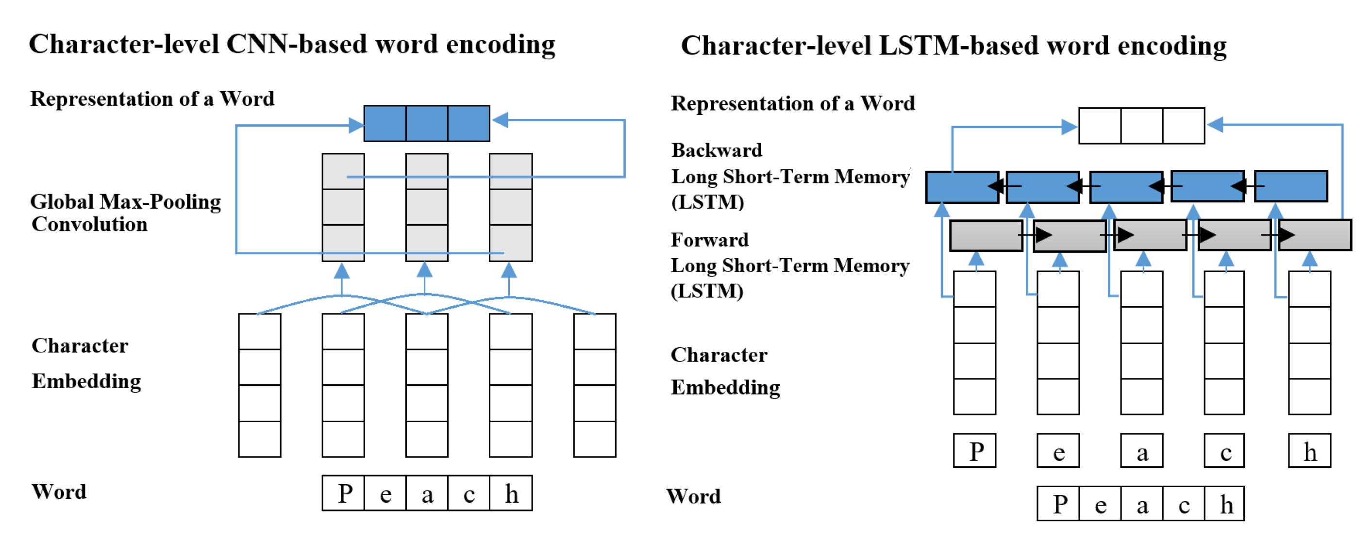
38]. Therefore, we also select these representations due to the same reason as well as the importance of character information in NER task. There are two standard architectures for learning word encoding based on character embedding: CNN and LSTMs.
Ma and Hovy [
3] fed the character embeddings into the CNN with 30 filters of size three followed by global max pooling to get the encoding of the corresponding word. Lample et al. [
2] passed the character embeddings through forward and backward LSTMs and concatenated each outputs to get the encoding of the corresponding word, as shown in
Figure 1.
We adapted hyper-parameter values such as the number of filters, filter size, max word length and word encoding dimension from the previous works and the detailed values are given in
Section 4.2.
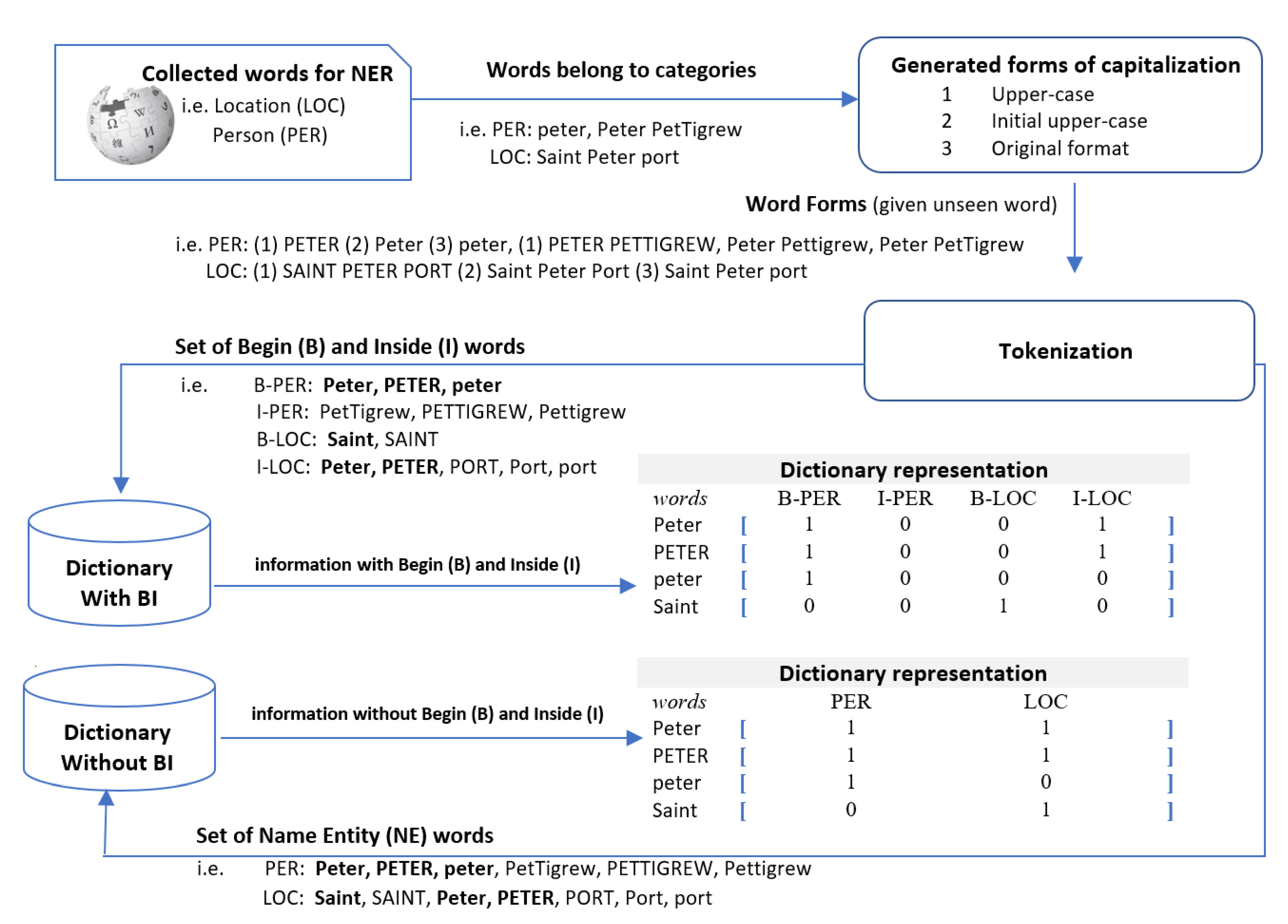
4. CNN-based Dictionary Representation: We first build up two versions of the NE dictionary for partial matching: one distinguishes the begin and inside words in a named entity and the other does not distinguish them. The process of dictionary creation consists of four sequential steps, as follows: (1) we gather named entities of eleven types—Person, Location, Norp, Facility, Organization, Product, Event, Work of art, Law, Language and a geopolitical entity (GPE)—from Wikipedia, Kaggle, and Geonames. Then, (2) we additionally generate all upper-cased names and initial upper cased names from the collected names. As a result, we could reduce mismatches when we apply a cased match. Subsequently, (3) we duplicate the dictionary and tokenize these entries, as follows.
Dictionary without a Begin-Inside Tag: We tokenize each word in the vocabularies and classify each word into an entity type based on the datasets (CoNLL 2003, OntoNotes 5.0).
Dictionary with a Begin-Inside Tag: we tokenize each names in the list and classify each word based on the word position as well as the entity types. The first word in an entity has ‘Begin-tag’ along with the entity type and the other words in the entity have ‘Inside-tag’ along with the entity type.
Now, we obtain two kinds of dictionaries with tokenized words. Finally, (4) we merge entity types along with Begin-Inside tags for each word and construct a matrix of word to possible entity types using binary notation. That is, we set to 1 when a word occurred at least once as that type in the list of names and set to 0 otherwise, as shown in
Figure 2.
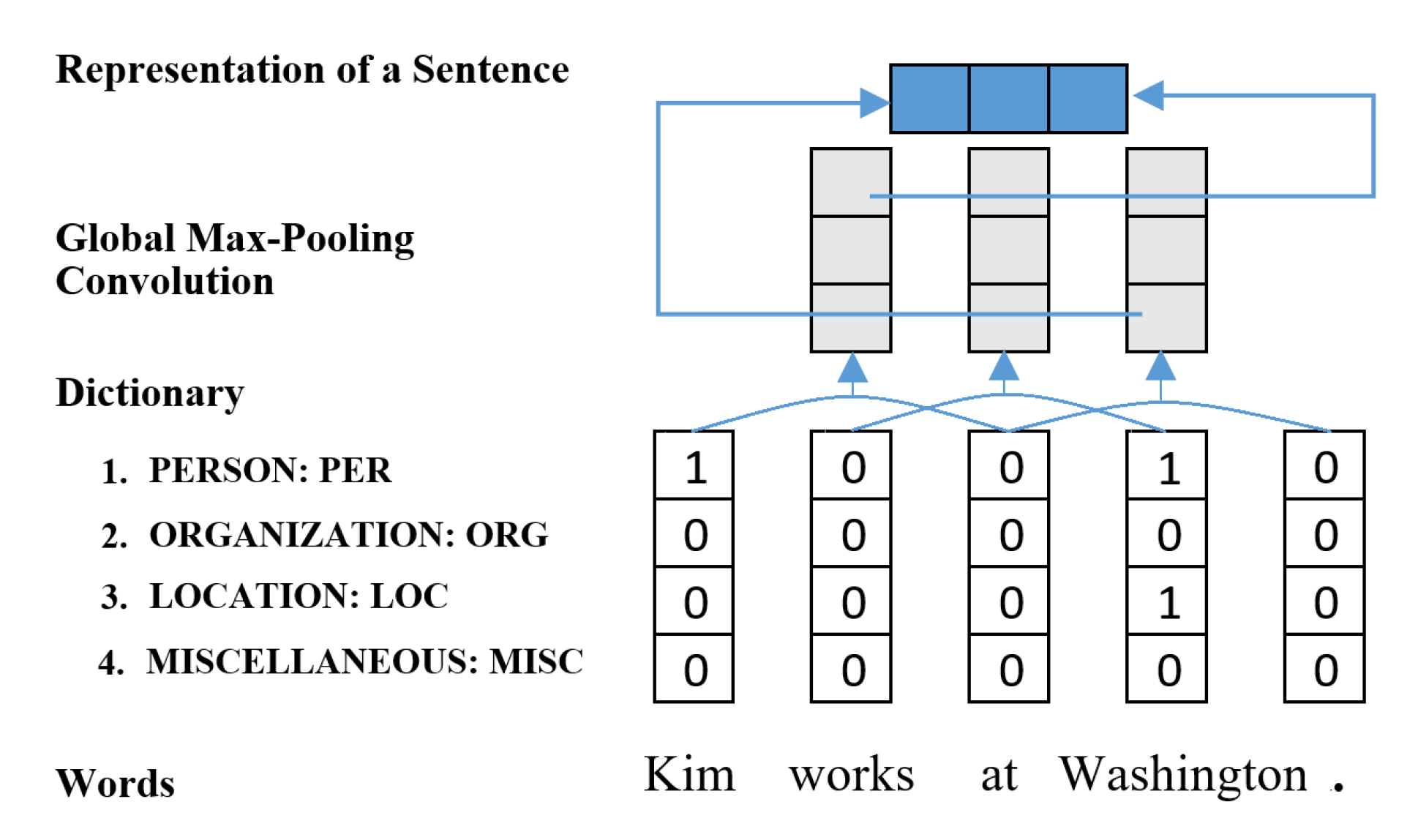
This dictionary is used for encoding each sentence by the CNN with 30 filters of size three and followed by global max pooing. Our dictionary employs partial match strategy, which may cause many false matches and give negative effect on the performance. To soften this problem, we applied CNN-based sentence encoding, as shown in
Figure 3, and combined this with the output of the bidirectional LSTM blocks, instead of early combining with other feature encodings at the embedding layer.
This representation also has the advantage in dealing with ungrammatical or non-contextual short sentences, which often occur in the dataset due to incorrect sentence segmentation but could not be correctly predicted using only context.
3.2. Delayed Combination
We selected or designed four kinds of feature encodings, which are promising for NER task: pre-trained word embedding, contextual embedding, character-level CNN/LSTM-based word encoding and CNN-based sentence encoding using a dictionary. These feature encodings are combined at suitable positions of the bidirectional LSTM CRF network according to the characteristics of each feature encoding.
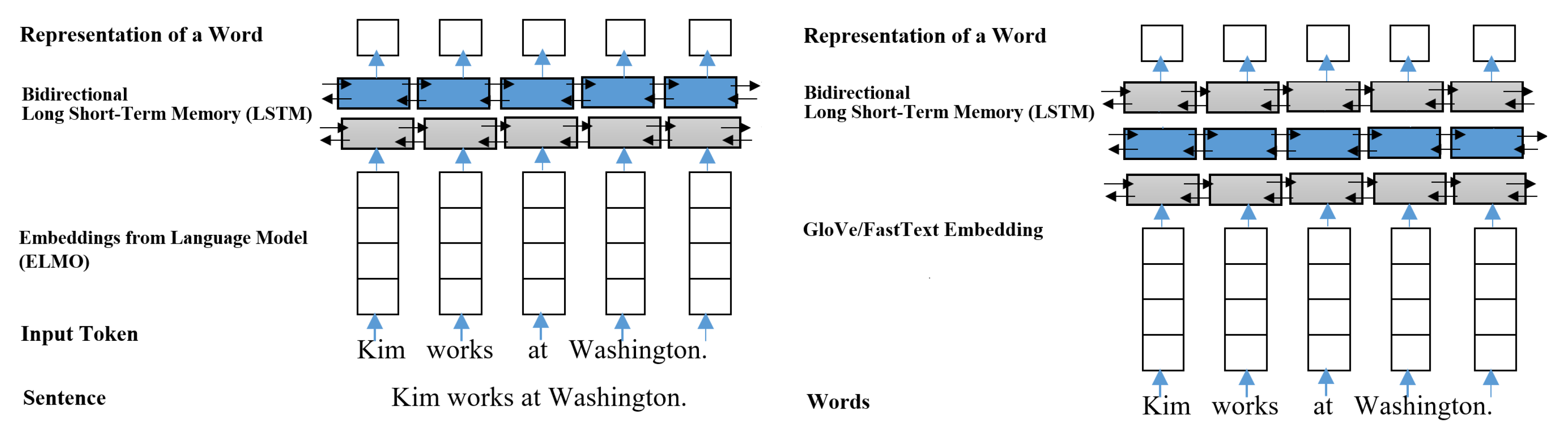
The pre-trained word embedding and contextual embedding were learned from the context of each word. That is, their major role is to maintain and propagate the contextual information of each word to the latter layers. So we decided to pass both of them through each separate bidirectional LSTM blocks to further learn or fine-tune the contextual information from the training data as shown in
Figure 4.
On the contrary, character-level CNN/LSTM-based word encoding is better to bypass the bidirectional LSTM blocks because this word encoding learns only the character compositions within a word, not contextual information of a word. Passing this encoding through the bidirectional LSTM blocks may cause loss of character composition information in that encoding. Early combination of this encoding with other pre-trained feature encodings at the embedding layer may disturb correct learning of that encoding because in general dominant features (i.e., pre-trained ones) are first propagated to the latter layers.
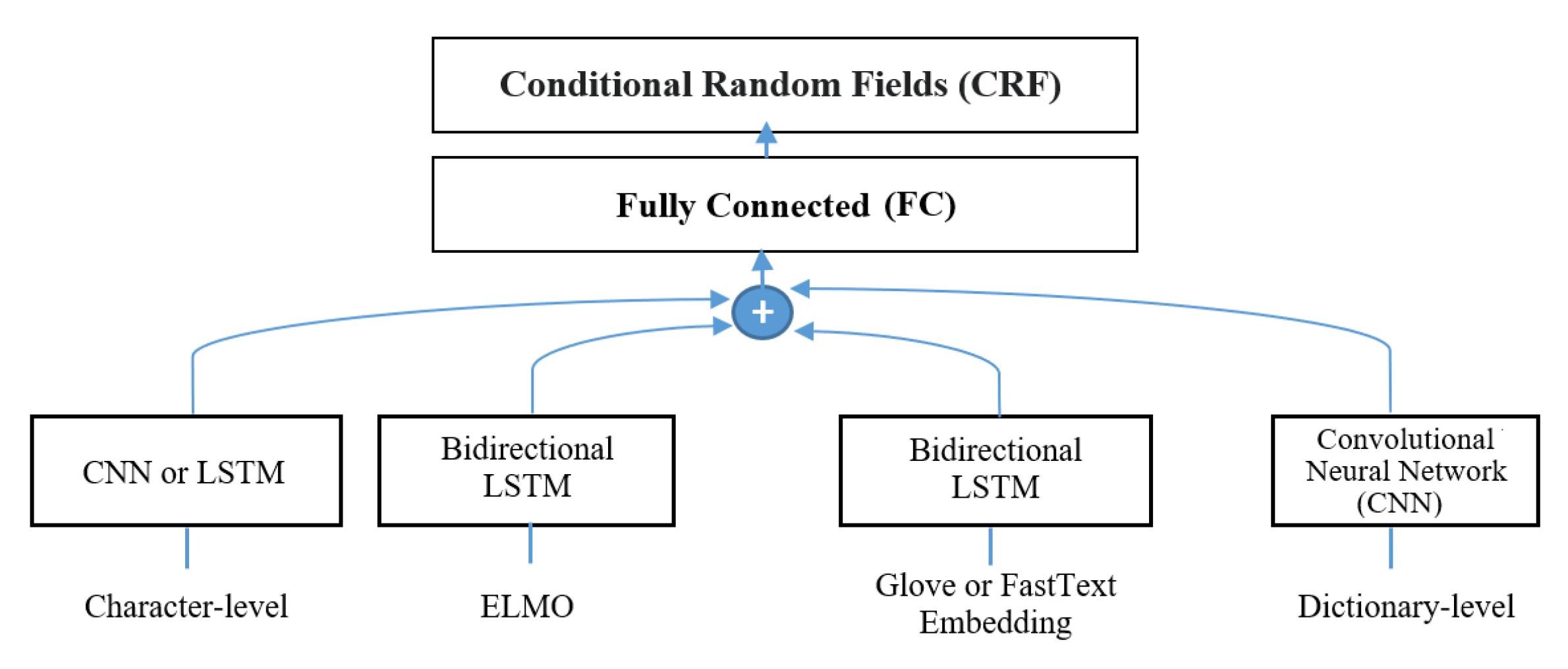
Our dictionary representation is also not passed through the bidirectional LSTM blocks. The representation is obtained by employing a partial match strategy and passing through word CNN. This partial match may cause many false matches and give a negative effect on the performance. To soften this problem, we employed CNN-based sentence encoding. As a result, we combine (i.e., concatenate) the above feature encodings at the fully-connected layer directly after the bidirectional LSTM blocks. The combined encoding further passes fully-connected layer and CRF layer to find the best chainable label sequences. A graphical illustration of our delayed combination model is given in
Figure 5.
The early combination may cause some useful information to mix or collide with other encodings and, as a result, disappear before the output layer. The graphical difference between the early combination and the delayed combination is depicted in
Figure 6.
Both the delayed combination and early combination models are used for comparison in experiments, as explained in the next section.
4. Experimental Setup
4.1. Datasets
The experiment begins by exploring the NER datasets. The CoNLL 2003 dataset (English language) [
39], was taken from Reuters news corpus between August 1996 and 1997. This dataset consists of four types of named entities (i.e., person, location, organization, and miscellaneous). The number of occurrences of each type of named entity is shown in
Table 1. The dataset consisted of three parts: a training set, a development set, and a test set. To be specific, the training and development datasets were collected from the news at the end of August of 1996, while the test dataset was obtained from the news in December of 1996.
OntoNotes 5.0 is made up of 300 K Arabic, 900 K Chinese, and 1745 K English text data instances and covers six types of documents such as newswire, websites, broadcasting news, broadcasting conversation, magazine and telephone conversation [
40]. It consists of eleven types of named entity and seven types of values and we use the English data and follow the train–validate–test split by [
40]. We excluded the telephone conversation section when evaluating our model because it has quite noisy annotations. The detailed statistics of this dataset are given in
Table 2.
We selected these two datasets for benchmarking our model because they have been most actively used for evaluating and comparing NER models until now even though they are a little old. Especially, CoNLL 2003 is a little small and so takes less time to train a model. So, it is suitable for testing and tuning model feasibility at the early stage.
On the contrary, OntoNotes 5.0 is quite large (about five times the size of CoNLL 2003 in the number of sentences in the training set) and has manymore types of named entities. So, it is suitable for testing model extensibility at the latter stage.
4.2. Hyperparameter Setup
As preliminary experiments, we explored the optimal values of several major hyper-parameters such as dropout, optimizer with learning rate, and the number of bidirectional LSTM layers and also tested several versions of the popular pre-trained word embeddings including GloVe and FastText (More detailed information is given in the
Appendix A). The other hyper-parameter values were borrowed from the earlier works [
2,
3,
4,
5,
33].
Table 3 shows the hyper-parameter values used in our experiments. The hyper-parameter values are nearly identical between CoNLL 2003 and OntoNotes 5.0, except for the maximum word length and character embedding dimension, which were borrowed from the earlier studies [
2,
5], respectively.
4.3. Model Setup
When training our models, we used two different numbers of iterations without early stopping: (1) 200 epochs for all model variants except the model with ELMo and (2) 120 epochs for the model with ELMo. This is because the performance of the model with ELMo was rarely improved but the model took quite a long time in training at each epoch when further increasing the number of epochs.
We evaluated our model after every epoch with the F1 score on the validation set and selected the best validation F1 scored model within the number of epochs, which was used for evaluating the test set. Due to the randomness, we did the same experiments five times and averaged them. The following equation calculates the F1 score:
Here, precision refers to the ratio of correct named entities found in the NER system, and recall is the ratio of named entities that are retrieved by the NER system. Our goal is to show the effectiveness of the delayed combination and the CNN-based sentence encoding using the dictionary. To achieve this goal, we organized three groups of experiments as follows:
The experiments for comparison between the delayed and the early combinations of FastText (FT) and character-level CNN or LSTM word encoding (we refer to these as Delayed-BiLSTM-CRF (FT + CNN or LSTM) and Early-BiLSTM-CRF (FT+ CNN or LSTM), respectively). The results are given in
Section 5.1.
The experiments with the model equipped with our dictionary representation (we refer to this model as Delayed-BiLSTM-CRF (FT + CNN or LSTM + Dic)). The results are given in
Section 5.2.
The experiments with the model additionally equipped with ELMo encoding (we refer to this model as Delayed-BiLSTM-CRF (FT + CNN or LSTM + Dic + ELMo)). The results are given in
Section 5.3.
5. Results and Discussion
5.1. Comparison between the Delayed and Early Combination Models
In this experiment, we first compared the delayed combination to the early combination by evaluating our own implementations of both combinations on CoNLL 2003 and OntoNotes 5.0. We used FastText for the pre-trained word embedding and character-level CNN-based word encoding. In the early combination, both were concatenated at the embedding layer, and then fed into the bidirectional LSTM blocks. On the contrary, in the delayed combination, only the FastText encoding was passed through the bidirectional LSTM blocks and then the output was concatenated with the character-level CNN-based word encoding. The results are shown in
Table 4.
We can see that the delayed combination (Delayed-BiLSTM-CRF (FT + CNN)) gives consistently and significantly higher scores than the early combination (Early-BiLSTM-CRF (FT + CNN)) on both datasets. This could convince us that the delayed combination could effectively propagate the useful character composition information to the output layer by bypassing the bidirectional LSTM blocks. The bidirectional LSTM blocks are very good at learning contextual information but the character composition information may diminish or disappear when it passes through the bidirectional LSTM blocks. Furthermore, at the early stage of the training, the pre-trained word embedding has more dominant values than the character-level word encoding, which is randomly initialized. This means that the early combination of feature encodings having different characteristics could hinder the model from learning the less dominant feature encodings especially at the early stage of the training.
Reimer et al. [
41] described the difference between character-level CNN-based and LSTM-based word encoding approaches. According to this work, the CNN approach takes only the trigram value into account but cannot distinguish the positions of trigrams, i.e., whether it is at the beginning, inside, or at the end of a word. In contrast, the LSTM approach takes all characters of a word into account and can distinguish between characters at the beginning and end of a word.
Referring to this work [
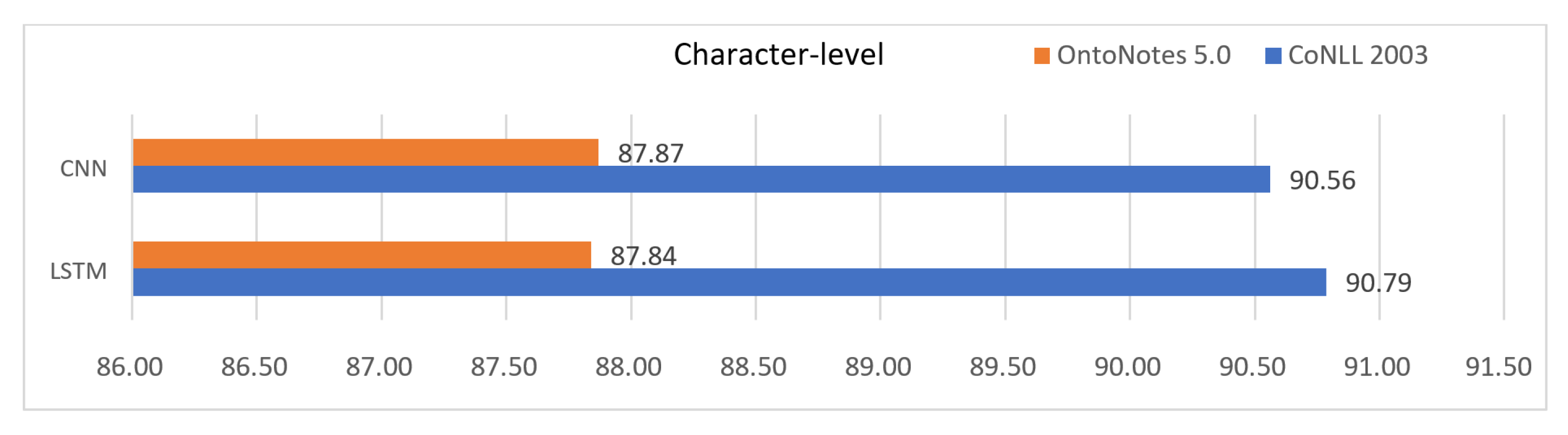
41], we compared the two kinds of character-based word encoding approaches in our delayed combination model. The result is given in
Figure 7. On the CoNLL 2003 dataset, the LSTM approach was distinctly better (about +0.23%) than the CNN approach. However, on the OntoNotes 5.0 dataset, the CNN approach was very slightly better (about +0.03%) than the LSTM approach. This means that we cannot say which one is definitely better than the other. This result coincides with the results from the previous works [
30]. We also checked the computation time in the training of each approach. The LSTM approach took about 1.75 times longer training time than the CNN approach. This means that the CNN approach has advantage in the view of the training speed. From these results, we decided to fix the approach for character-level word encoding to LSTM on the CoNLL 2003 dataset and CNN on the OntoNotes 5.0 dataset, respectively.
To show the feasibility of our own model, we show in
Table 5 the comparison between the results of our models and the results of the previous works having similar model architecture and combining features at the embedding layer. Our delayed model with LSTM-based word encoding, Delayed-BiLSTM-CRF (LSTM), could achieve a better F1 score than the results from Rei et al., 2016, Ghaddar and Langlais, 2018 and Le and Burtsev, 2019, but worse F1 score than the original results from Lample et al., 2016, Ma and Hovy, 2016 and Chiu and Nichols, 2016 on the CoNLL 2003 dataset. However, when comparing to the re-implementation results by DeLFT [
42] of the latter three works, our results were not worse. On the OntoNotes 5.0 dataset, our model was also better than the results from Ghaddar and Langlais, 2018 and Chiu and Nichols, 2016. We did not tune the most hyper-parameter values and just borrowed from the previous works. We think our model is open to be further improved by thoroughly tuning the hyper-parameter values [
41].
5.2. The Model Equipped with Our Dictionary Representation
Before evaluating our model with dictionary representation, we first checked the coverage of the collected list of named entities on the two target datasets to assess whether collected names are enough or not for the datasets. The coverages by each named entity (NE) type of CoNLL 2003 and OntoNotes 5.0 are given in
Table 6 and
Table 7, respectively.
The percentage in the tables indicates that those ratios of named entity tokens of each type were found in the collected dictionary. On the CoNLL 2003, the dictionary covers well the first three types of names but only a small ratio of miscellaneous typed entities is covered. On the OntoNotes 5.0 dataset, only four types of names such as Person, Facility, Organization and GPE are well covered (i.e., over 50%).
As explained in
Section 3.1, we built up two kinds of dictionaries: one distinguishes begin and inside tokens in a named entity while the other does not. After combining this dictionary feature with our model at the delayed position, we evaluated our model to show the effectiveness of the dictionary feature.
Table 8 shows the comparison of our models with and without the CNN-based dictionary representation and also compares the two kinds of dictionaries with or without Begin-Inside (BI) tags. On the CoNLL 2003, both of the two dictionary representations (with and without BI tags) could improve significantly the F1 score by +0.34% and +0.45%, respectively. On the OntoNotes 5.0, the dictionary without BI tags could improve the F1 score by +0.20% although the dictionary representation with BI tags rather lowered the F1 score by −0.30%.
From this result, we could say that the CNN-based dictionary representation could improve the F1 score. Further analysis lets us find that our dictionary effectively classified the type of a word especially when the context of the word is not sufficient. For example, the named entities in one-word sentences (e.g., ‘England’), which are often found on CoNLL 2003 dataset, cannot be correctly predicted only using the Recurrent Neural Network (RNN)-typed network because they have no contextual information [
43]. However, our CNN-based dictionary representation could predict them correctly.
Commonly on the two datasets, we can notice that the dictionary without BI tags shows a better F1 score. We think this result might be caused by the following two reasons: tag mismatches and many ambiguous words. First, the ‘tag mismatches’ are very often found in between the dictionary with BI tags and the CoNLL 2003 dataset, especially for Person. We may think that a given name of a person is generally classified with a begin tag, whereas a family name is typically assigned with an inside tag. However, in the dataset of real text, it is very common to refer to a person by only his/her family name without giving a given name. So, family names are assigned both begin and inside tags in the dataset. The most collected names were in the full form of names and the dictionary made from them often caused such tag mismatches and, as a result, degraded the performance.
Secondly, the ‘ambiguous words’ are very often found in the dictionary with BI tags for OntoNotes 5.0. For example, ‘Hong’ is a word found in various named entities, such as FACILITY: ‘Hong Kong International Airport’, GPE: ‘Hong Kong’, EVENT: ‘Hong Kong Jewish Film Festival’, WORK_OF_ART: ‘Hong Kong Garden’, PERSON: ‘Hong Chang’, ‘Chin Hong Goh’, LOCATION: ‘Disney Hong Kong’. When building the dictionary with BI tags up, ‘Hong’ is classified with B-FACILITY, B-GPE, B-EVENT, B-WORK_OF_ART, B-PERSON, I-PERSON, and I-LOCATION tags. This information is used to create a dictionary representation of the word ‘Hong’. Like this, many ambiguous words are incorrectly encoded into dictionary representations, among which some adjacent dictionary representations may form unseen patterns that never occurred in the training set but that could be found in the test set. As a result, those representations may pose a problem in that they drastically reduce the performance. This result is similar to that in the earlier work [
44].
We also compared our model to the previous similar dictionary-enabled works to show the feasibility of our model. The comparison is given in
Table 9. On the CoNLL 2003, our model could achieve a better F1 score than that of Huang et al., 2015 and Wu et al., 2018 but was worse than that of Chiu and Nichols, 2016 and Ghaddar and Langlais, 2018. However, Chiu and Nichols, 2016 trained their model by merging the validation data with the training data and this could lead to improve the F1 score. Ghaddar and Langlais, 2018 used the lexical similarity (LS) embedding which was pre-trained from fined-grained named entity list and Wikipedia text. The LS embedding was well-organized than the existing dictionaries and could lead to improve the F1 score by +1.21%.
In contrast, the OntoNotes 5.0 dataset, our model could achieve better F1 score than those of Chiu and Nichols, 2016 and Ghaddar and Langlais, 2018 even though Chiu and Nichols, 2016 used both training and validation data for training their model and Ghaddar and Langlais, 2018 applied the LS embedding.
5.3. The Model Additionally Equipped with the ELMO Encoding
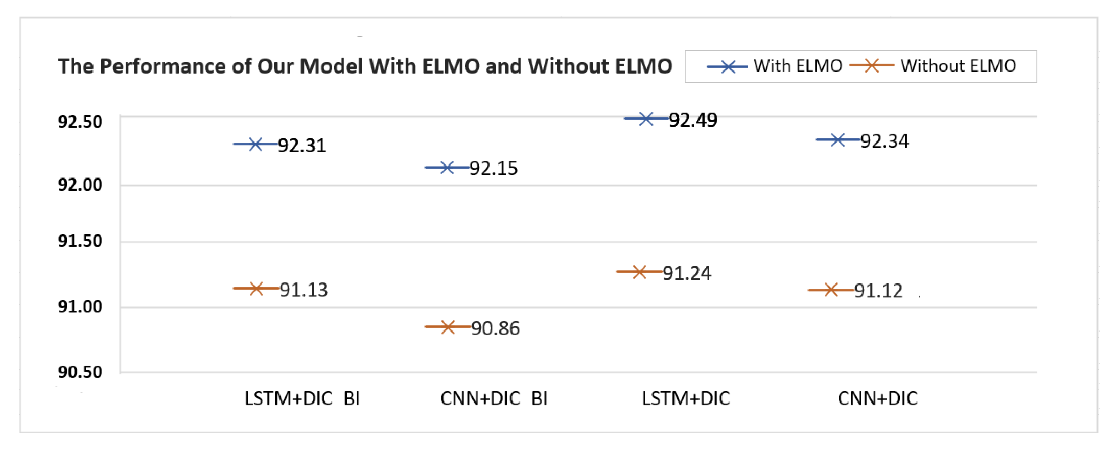
Our model is finally combined with the separate bidirectional LSTM network of the ELMo embedding at the delayed position (The OntoNotes5.0 dataset couldn’t be used for training our model with ELMo encoding because high-end GPUs like V100 were not available within a limited duration.). On the CoNLL 2003 dataset, we checked the effect of the ELMo encoding on all variants of our model according to all possible combinations with the two kinds of character-level word encodings and the two kinds of dictionary representations.
The result is shown in
Figure 8. Our model could achieve the highest F1 score, 92.49%, when we combined our model with LSTM-based word encoding, dictionary representation without BI tags, and the bidirectional LSTM-based ELMo encoding. The bidirectional LSTM-based ELMo encoding could consistently improve the F1 score of all four variants of our model by the range of [+1.12%, +1.29%].
We also compared our model equipped with the ELMo encoding to the previous works having contextual embedding as features of their models. This is given in
Table 10. Our model could achieve a better F1 score than all the previous works used ELMo as one of their features, such as Peter et al., 2018, Han et al., 2019, Xia et al., 2018, and Jie and Lu, 2018. This result could convince us that our delayed combination model is effective in NER task. Our model still shows a little higher F1 score than the model used BERT-Base (Devlin et al., 2019) but other previous works used BERT-Large or further tuned LM embedding still outperform our model. We think that our model can be further improved by combining with BERT-Large or fine-tuned LM embeddings instead of ELMo.
6. Conclusions and Future Works
For the success of various deep-learning methods in NER task, most researchers have tested various feature-encoding techniques such as pre-trained word embedding, contextual embedding, character-level CNN or LSTM-based word encoding, word pattern-based encoding and dictionary-based encoding, and incorporated them into the deep learning networks. When more than one feature encoding is used, most previous works combined them at the embedding layer and then passed through the deep neural network to find the best label sequences in the output layer. However, when such an early combination of various feature encodings passes through the deep neural networks like RNN, much useful information could be mixed or shrunk by other more-dominant information and this could consequently limit the improvement in performance.
To avoid such limitations, we introduced the delayed combination model of various promising feature encodings. This model selected FastText as the pre-trained word embedding, ELMo as the contextual embedding and character-level CNN or LSTM word encoding, and designed CNN-based sentence encoding using a dictionary, for feature encoding. We also selected the most common bidirectional LSTM network for learning contextual information from the train set. Among those feature encodings, FastText and ELMo embeddings were passed through its own separate bidirectional LSTM blocks while the remaining feature encodings were bypassed and combined with the outputs of the bidirectional LSTM blocks.
Through several experiments, we showed that our delayed combination model outperforms the early combination one and also showed the feasibility of our model by comparing our results with the corresponding previous works.
As future work, we intend to extend this model by (1) building up a dictionary better-organized and learned from the external resources, (2) incorporating BERT-Large or other fine-tuned LM embeddings into our model, and applying to other non-English languages as well as other fine-grained NER task.
Author Contributions
Conceptualization, S.L. and C.R.; methodology, C.R.; software, C.R.; validation, S.L., H.J.J. and C.R.; formal analysis, C.R.; investigation, H.J.J.; resources, H.J.J and C.R.; data curation, C.R.; writing—original draft preparation, C.R; writing—review and editing, S.L. and H.J.J; visualization, C.R.; supervision, S.L.; project administration, S.L.; funding acquisition, S.L. All authors have read and agreed to the published version of the manuscript.
Funding
This research was funded by Government-wide R&D Fund project for infectious disease research (GFID), Korea, under grant number HG18C0093.
Conflicts of Interest
The authors declare no conflict of interest.
Appendix A. The Hyperparameters Tuning
Reimer et al. [
41] noted that there is a high impact of hyper-parameters (dropout, optimizer, word embedding, and a number of stacked layers) on the accuracy of the bidirectional LSTM CRF. We used the two-stacked bidirectional LSTM CRF model to find optimal hyper-parameters of dropout, optimizer, and word embedding. Hyper-parameter tuning is discussed in the four subsections below.
Dropout
Dropout is a technique that can be used to reduce over-fitting and to improve the model’s performance [
51,
52,
53]. Brownlee [
54] suggested that “normally, a small dropout value of 0.2–0.5 of neurons gives a good starting point.” For our dropout experiment, dropouts were applied to three positions: (1)
inside the bidirectional LSTM layer within a recurrence loop, (2)
after the last output values of the bidirectional LSTM layer, and (3)
before the outputs are passed through the CRF layer.
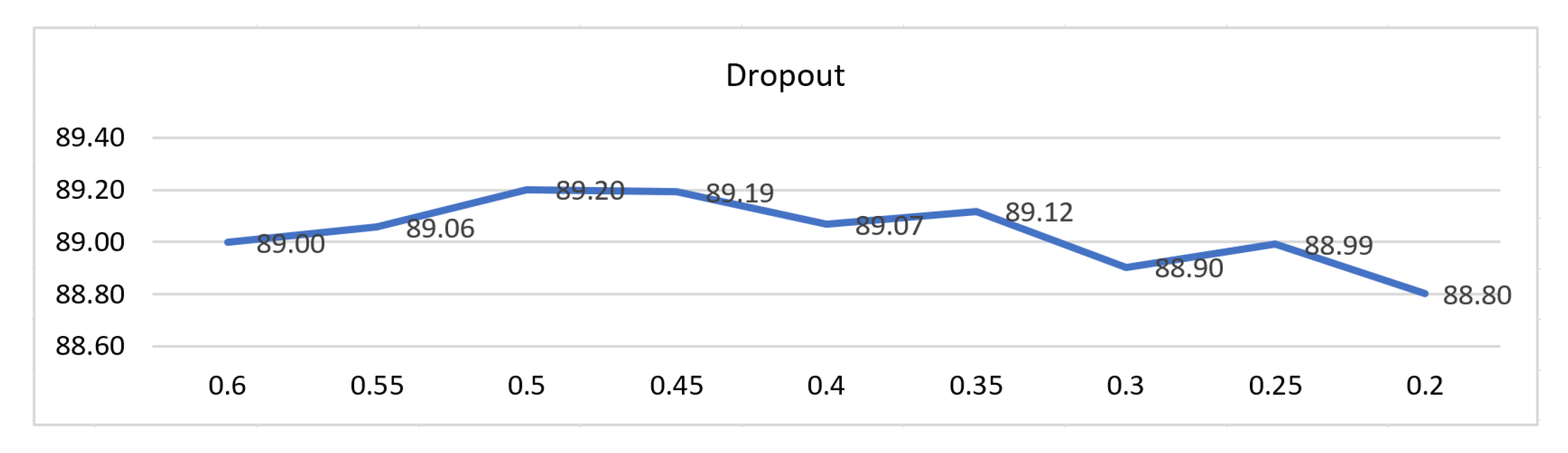
The
Figure A1 shows the experiment with different dropout sets. We repeat the experiment five times with different random seeds seeds and averaged them. The dropout value 0.5 of neurons provides our best result. The resulting rate is similar to that in the earlier work by Srivastava et al., 2014 [
51], suggesting that the 0.5 dropout is be close to the optimal value for a wide range of neural networks and multiple tasks.
Figure A1.
F1 score on NER with difference dropouts. The dropout value of 0.5 achieves the best score in this task (CoNLL 2003).
Figure A1.
F1 score on NER with difference dropouts. The dropout value of 0.5 achieves the best score in this task (CoNLL 2003).
Optimizer with learning Rate
The optimizer determines the impact of the gradients on the parameter that we study the optimizers [
55] (SGD, Adam, Nadam, RMSProp, and Adagrad) with variant learning rates that are derived from default values provided by Keras (
https://keras.io/api/optimizers). In particular, we utilize the set of 0.009, 0.01, 0.02, 0.03, 0.04 for SGD and Adagrad and the set of 0.0009, 0.001, 0.002, 0.003, 0.004 for Adam, Nadam, RMSprop and Adamax.
Table A1 shows the optimizers’ performance with various learning rates on the CoNLL 2003 and OntoNotes 5.0 datasets. The dropout was fixed at 0.5.
For CoNLL 2003, the average performances of Nadam and Adagrad are first and second highest and achieve rates 89.321% and 89.316%, respectively. In another observation, Adamax(lr = 0.001) shows the best rate at 89.50%. However, it is only 0.01 different from Nadam(lr = 0.002). Earlier work [
41] claims that Nadam converges most rapidly. It requires only a small training epoch to achieve better performance. Therefore, we used Nadam with a learning rate of 0.002 and a 0.5 dropout value for the next experiment on the CoNLL 2003 dataset.
Table A1.
Five times F1 scores of the optimizer, in this case SGD, Adam, Nadam, RMSprop, Adagrad, and Adamax.
Table A1.
Five times F1 scores of the optimizer, in this case SGD, Adam, Nadam, RMSprop, Adagrad, and Adamax.
| | | Learning Rate Multiplied by Alpha () | | |
|---|
| Dataset | Mini-Batch | Optimizer () | 0.09 | 0.1 | 0.2 | 0.3 | 0.4 | Average | SD * |
|---|
| Conll 2003 | 200 | SGD ( =0.1 ) | 89.40 | 89.18 | 89.34 | 89.12 | 89.12 | 89.232 | 0.13 |
| | | Adam ( =0.01) | 89.17 | 89.23 | 89.45 | 89.17 | 88.94 | 89.190 | 0.18 |
| | | Nadam ( =0.01) | 89.17 | 89.39 | 89.49 | 89.34 | 89.22 | 89.321 | 0.13 |
| | | RMSprop ( =0.01) | 89.09 | 89.11 | 89.30 | 89.30 | 89.06 | 89.172 | 0.12 |
| | | Adagrad ( =0.1) | 89.14 | 89.48 | 89.40 | 89.23 | 89.34 | 89.316 | 0.13 |
| | | Adamax ( =0.01) | 89.24 | 89.50 | 89.27 | 89.34 | 89.21 | 89.313 | 0.12 |
| OntoNotes 5.0 | 200 | Nadam ( =0.01) | 86.78 | 87.08 | 86.83 | 86.28 | 86.03 | 86.599 | 0.43 |
An earlier experimental result [
41] related to our CoNLL 2003 experiment recommends Nadam as an optimal hyper-parameter. For OntoNotes 5.0, we study the effect of Nadam with various learning rates. From the result in
Table A1 the 0.001 learning rate provided our best F1 score. Accordingly, we chose Nadam(lr = 0.001) as an optimal hyper-parameter for the next experiment on the OntoNotes 5.0 dataset.
Pre-trained Word Embedding
We compared the GloVe 840B embedding and FastText–cc.en.300.vec and cc.en.300.bin. For FastText, the experiment used two options: (1) cc.en.300.vec (without subwords), (2) cc.en.300.bin (with subwords).
In this experiment, each pre-trained embedding was used to convert any word from the target dataset for representation and to pass it through the two-stacked bidirectional LSTM CRF model for predicting the named entity tags.
Table A2 shows the experimental results of CoNLL 2003 and OntoNotes 5.0.
Table A2.
Five times F1 scores of the pre-trained word embedding with two-stacked bidirectional LSTM. From the result, we achieve the best F1 score when using FastText with subwords.
Table A2.
Five times F1 scores of the pre-trained word embedding with two-stacked bidirectional LSTM. From the result, we achieve the best F1 score when using FastText with subwords.
| | | Five Times Validation | | |
|---|
| Dataset | Mini-Batch | Embedding | 1 | 2 | 3 | 4 | 5 | Average | SD |
|---|
| Conll 2003 | 200 | GloVe | 89.96 | 89.90 | 89.94 | 90.26 | 90.24 | 90.06 | 0.18 |
| | | FastText Vec | 89.44 | 89.70 | 89.79 | 89.44 | 89.93 | 89.66 | 0.22 |
| | | FastText Bin | 90.05 | 90.30 | 90.20 | 89.97 | 90.17 | 90.14 | 0.13 |
| OntoNotes 5.0 | 200 | GloVe | 87.12 | 87.44 | 87.42 | 87.42 | 87.61 | 87.40 | 0.18 |
| | | FastText Vec | 87.49 | 87.49 | 87.44 | 87.52 | 87.40 | 87.47 | 0.05 |
| | | FastText Bin | 87.68 | 87.43 | 87.74 | 87.58 | 87.58 | 87.60 | 0.12 |
The results from the CoNLL 2003 dataset show that the average F1 score of FastText (90.14%) with subwords higher than that of the GloVe (90.06%) experiment. For OntoNotes 5.0 experiment, the result is similar to that of CoNLL 2003. The F1 score (at 87.60%) is increased when using FastText with subwords.
Owing to the similar result on the two datasets, we assume that the model performance is improved when (1) the vocabulary in word embedding matches the word in the dataset, and (2) the subword (n-gram) of FastText is used to generate embeddings for rare words.
Number of bidirectional LSTM layers
Currently, the stacked LSTMs are used as a standard technique for challenging sequence predictions [
56]. Some previous works [
57,
58,
59] present the multiple stacked bidirectional LSTMs in a neural network. They show that the classification performance can be improved when using this technique. Furthermore, there is some related theoretical support: a deep hierarchical model is more effective at representing than a shallow model [
30,
60]. Due to the stacked processes, when the first bidirectional LSTM layer provides an output vector, this output vector provides more complex patterns for the next layer, enabling us to capture information on a different scale.
Cai et al. [
57] suggests the appropriate amount of multi-layer bidirectional LSTM help to understand the relationship between words and words at a deep level. However, when the representation flows through stacked layers, the risk arises that the representation information will be lost [
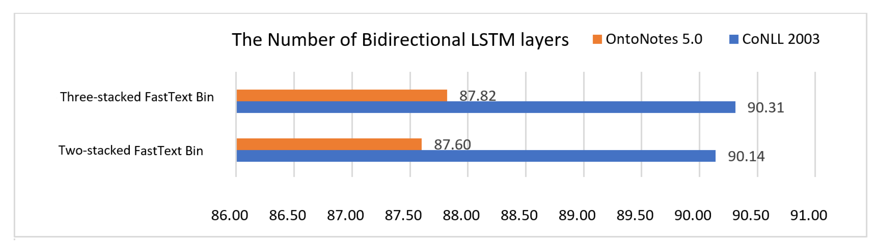
61], and it may also reduce the model performance. Hence, we examined two or three-stacked bidirectional LSTM to find the number of layers most suitable for our model. The comparative of F1 score results are shown in
Figure A2 the model shows higher performance when using the three-stacked bidirectional LSTM. Consequently, we assume that three stacks are able to capture more information for our model.
In contrast, two-stacked bidirectional LSTMs are applied in earlier experiments [
2,
23,
35]. However, these experiments used different batch sizes, optimizers and lower dimensional word embedding compared to our model. Accordingly, we assume that the number of bidirectional layers depends on the hyper-parameters, especially the input size, batch size, optimization and hidden unit [
62] of each model.
Figure A2.
Comparison between two and three stacked bidirectional LSTM CRFs. The results show that three stacked bidirectional LSTM CRFs perform well on both CoNLL 2003 and OntoNotes 5.0.
Figure A2.
Comparison between two and three stacked bidirectional LSTM CRFs. The results show that three stacked bidirectional LSTM CRFs perform well on both CoNLL 2003 and OntoNotes 5.0.
References
- Li, J.; Sun, A.; Han, J.; Li, C. A Survey on Deep Learning for Named Entity Recognition. arXiv 2018, arXiv:1812.09449. [Google Scholar] [CrossRef]
- Lample, G.; Ballesteros, M.; Subramanian, S.; Kawakami, K.; Dyer, C. Neural architectures for named entity recognition. arXiv 2016, arXiv:1603.01360. [Google Scholar]
- Ma, X.; Hovy, E. End-to-end sequence labeling via bi-directional lstm-cnns-crf. arXiv 2016, arXiv:1603.01354. [Google Scholar]
- Rei, M.; Crichton, G.K.; Pyysalo, S. Attending to characters in neural sequence labeling models. arXiv 2016, arXiv:1611.04361. [Google Scholar]
- Chiu, J.P.; Nichols, E. Named entity recognition with bidirectional LSTM-CNNs. Trans. Assoc. Comput. Linguist. 2016, 4, 357–370. [Google Scholar] [CrossRef]
- Huang, Z.; Xu, W.; Yu, K. Bidirectional LSTM-CRF models for sequence tagging. arXiv 2015, arXiv:1508.01991. [Google Scholar]
- Khattak, F.K.; Jeblee, S.; Pou-Prom, C.; Abdalla, M.; Meaney, C.; Rudzicz, F. A survey of word embeddings for clinical text. J. Biomed. Inform. X 2019, 4, 100057. [Google Scholar] [CrossRef]
- Mikolov, T.; Chen, K.; Corrado, G.; Dean, J. Efficient estimation of word representations in vector space. arXiv 2013, arXiv:1301.3781. [Google Scholar]
- Le, Q.; Mikolov, T. Distributed representations of sentences and documents. arXiv 2014, arXiv:1405.4053. [Google Scholar]
- Levy, O.; Goldberg, Y. Linguistic regularities in sparse and explicit word representations. In Proceedings of the Eighteenth Conference on Computational Natural Language Learning, Baltimore, MD, USA, 26–27 June 2014; pp. 171–180. [Google Scholar]
- Mikolov, T.; Sutskever, I.; Chen, K.; Corrado, G.S.; Dean, J. Distributed representations of words and phrases and their compositionality. arXiv 2013, arXiv:1310.4546. [Google Scholar]
- Mikolov, T.; Yih, W.t.; Zweig, G. Linguistic regularities in continuous space word representations. In Proceedings of the 2013 Conference of the North American Chapter of the Association for Computational Linguistics: Human Language Technologies, Atlanta, Georgia, 9–14 June 2013; pp. 746–751. [Google Scholar]
- Sugawara, H.; Takamura, H.; Sasano, R.; Okumura, M. Context representation with word embeddings for wsd. In Proceedings of the Conference of the Pacific Association for Computational Linguistics, Bali, Indonesia, 19–21 May 2015; pp. 108–119. [Google Scholar]
- Pennington, J.; Socher, R.; Manning, C.D. Glove: Global vectors for word representation. In Proceedings of the 2014 Conference on Empirical Methods in Natural Language Processing (EMNLP), Doha, Qatar, 25–29 October 2014; pp. 1532–1543. [Google Scholar]
- Du, M.; Vidal, J.; Al-Ibadi, Z. Using Pre-trained Embeddings to Detect the Intent of an Email. In Proceedings of the ACIT 2019: Proceedings of the 7th ACIS International Conference on Applied Computing and Information Technology, Honolulu, HI, USA, 29–31 May 2020. [Google Scholar] [CrossRef]
- Bojanowski, P.; Grave, E.; Joulin, A.; Mikolov, T. Enriching word vectors with subword information. Trans. Assoc. Comput. Linguist. 2017, 5, 135–146. [Google Scholar] [CrossRef]
- Almeida, F.; Xexéo, G. Word embeddings: A survey. arXiv 2019, arXiv:1901.09069. [Google Scholar]
- Peters, M.E.; Neumann, M.; Iyyer, M.; Gardner, M.; Clark, C.; Lee, K.; Zettlemoyer, L. Deep contextualized word representations. arXiv 2018, arXiv:1802.05365. [Google Scholar]
- Yang, Z.; Dai, Z.; Yang, Y.; Carbonell, J.; Salakhutdinov, R.R.; Le, Q.V. Xlnet: Generalized autoregressive pretraining for language understanding. arXiv 2019, arXiv:1906.08237. [Google Scholar]
- Liu, Y.; Ott, M.; Goyal, N.; Du, J.; Joshi, M.; Chen, D.; Levy, O.; Lewis, M.; Zettlemoyer, L.; Stoyanov, V. Roberta: A robustly optimized bert pretraining approach. arXiv 2019, arXiv:1907.11692. [Google Scholar]
- Sanh, V.; Debut, L.; Chaumond, J.; Wolf, T. DistilBERT, a distilled version of BERT: Smaller, faster, cheaper and lighter. arXiv 2019, arXiv:1910.01108. [Google Scholar]
- Collobert, R.; Weston, J.; Bottou, L.; Karlen, M.; Kavukcuoglu, K.; Kuksa, P. Natural language processing (almost) from scratch. J. Mach. Learn. Res. 2011, 12, 2493–2537. [Google Scholar]
- Zhai, Z.; Nguyen, D.Q.; Verspoor, K. Comparing CNN and LSTM character-level embeddings in BiLSTM-CRF models for chemical and disease named entity recognition. arXiv 2018, arXiv:1808.08450. [Google Scholar]
- Yang, Z.; Salakhutdinov, R.; Cohen, W. Multi-task cross-lingual sequence tagging from scratch. arXiv 2016, arXiv:1603.06270. [Google Scholar]
- Liu, L.; Shang, J.; Ren, X.; Xu, F.F.; Gui, H.; Peng, J.; Han, J. Empower sequence labeling with task-aware neural language model. In Proceedings of the Thirty-Second AAAI Conference on Artificial Intelligence, New Orleans, LA, USA, 2–7 February 2018. [Google Scholar]
- Eftimov, T.; Koroušić Seljak, B.; Korošec, P. A rule-based named-entity recognition method for knowledge extraction of evidence-based dietary recommendations. PLoS ONE 2017, 12, e0179488. [Google Scholar] [CrossRef]
- Jonnagaddala, J.; Jue, T.R.; Chang, N.W.; Dai, H.J. Improving the dictionary lookup approach for disease normalization using enhanced dictionary and query expansion. Database 2016, 2016, baw112. [Google Scholar] [CrossRef] [PubMed]
- Song, C.H.; Lawrie, D.; Finin, T.; Mayfield, J. Gazetteer generation for neural named entity recognition. In Proceedings of the Thirty-Third International Flairs Conference, North Miami Beach, FL, USA, 17–20 May 2020. [Google Scholar]
- Tsuruoka, Y.; Tsujii, J. Improving the performance of dictionary-based approaches in protein name recognition. J. Biomed. Inform. 2004, 37, 461–470. [Google Scholar] [CrossRef] [PubMed]
- Liu, Z.; Yang, M.; Wang, X.; Chen, Q.; Tang, B.; Wang, Z.; Xu, H. Entity recognition from clinical texts via recurrent neural network. BMC Med. Inform. Decis. Mak. 2017, 17, 67. [Google Scholar] [CrossRef] [PubMed]
- Gridach, M. Character-level neural network for biomedical named entity recognition. J. Biomed. Inform. 2017, 70, 85–91. [Google Scholar] [CrossRef] [PubMed]
- Wu, M.; Liu, F.; Cohn, T. Evaluating the utility of hand-crafted features in sequence labelling. arXiv 2018, arXiv:1808.09075. [Google Scholar]
- Ghaddar, A.; Langlais, P. Robust lexical features for improved neural network named-entity recognition. arXiv 2018, arXiv:1806.03489. [Google Scholar]
- Le, T.; Burtsev, M. A deep neural network model for the task of Named Entity Recognition. Int. J. Mach. Learn. Comput. 2019, 9, 8–13. [Google Scholar]
- Jie, Z.; Lu, W. Dependency-guided LSTM-CRF for named entity recognition. arXiv 2019, arXiv:1909.10148. [Google Scholar]
- Mikolov, T.; Deoras, A.; Povey, D.; Burget, L.; Černockỳ, J. Strategies for training large scale neural network language models. In Proceedings of the 2011 IEEE Workshop on Automatic Speech Recognition & Understanding, Waikoloa, HI, USA, 11–15 December 2011; pp. 196–201. [Google Scholar]
- Ilić, S.; Marrese-Taylor, E.; Balazs, J.A.; Matsuo, Y. Deep contextualized word representations for detecting sarcasm and irony. arXiv 2018, arXiv:1809.09795. [Google Scholar]
- Dong, G.; Liu, H. Feature Engineering for Machine Learning and Data Analytics; CRC Press: New York, NY, USA, 2018. [Google Scholar]
- Sang, E.F.; De Meulder, F. Introduction to the CoNLL-2003 shared task: Language-independent named entity recognition. arXiv 2003, arXiv:cs/0306050. [Google Scholar]
- Pradhan, S.; Moschitti, A.; Xue, N.; Ng, H.T.; Björkelund, A.; Uryupina, O.; Zhang, Y.; Zhong, Z. Towards Robust Linguistic Analysis using OntoNotes. In Proceedings of the Seventeenth Conference on Computational Natural Language Learning, Sofia, Bulgaria, 8–9 August 2013; Association for Computational Linguistics: Sofia, Bulgaria, 2013; pp. 143–152. [Google Scholar]
- Reimers, N.; Gurevych, I. Optimal hyperparameters for deep lstm-networks for sequence labeling tasks. arXiv 2017, arXiv:1707.06799. [Google Scholar]
- DeLFT. 2018–2020. Available online: https://github.com/kermitt2/delft (accessed on 30 July 2020).
- Frank, S.L. Strong systematicity in sentence processing by an echo state network. In Proceedings of the International Conference on Artificial Neural Networks, Berlin/Heidelberg, Germany, 10–14 September 2006; pp. 505–514. [Google Scholar]
- Ponomareva, N.; Thelwall, M. Biographies or blenders: Which resource is best for cross-domain sentiment analysis? In Proceedings of the International Conference on Intelligent Text Processing and Computational Linguistics, New Delhi, India, 11–17 March 2012; pp. 488–499. [Google Scholar]
- Han, K.; Chen, J.; Zhang, H.; Xu, H.; Peng, Y.; Wang, Y.; Ding, N.; Deng, H.; Gao, Y.; Guo, T.; et al. DELTA: A DEep learning based Language Technology plAtform. arXiv 2019, arXiv:1908.01853. [Google Scholar]
- Xia, C.; Zhang, C.; Yang, T.; Li, Y.; Du, N.; Wu, X.; Fan, W.; Ma, F.; Yu, P. Multi-grained named entity recognition. arXiv 2019, arXiv:1906.08449. [Google Scholar]
- Devlin, J.; Chang, M.W.; Lee, K.; Toutanova, K. Bert: Pre-training of deep bidirectional transformers for language understanding. arXiv 2018, arXiv:1810.04805. [Google Scholar]
- Luo, Y.; Xiao, F.; Zhao, H. Hierarchical Contextualized Representation for Named Entity Recognition. arXiv 2019, arXiv:1911.02257. [Google Scholar]
- Li, X.; Sun, X.; Meng, Y.; Liang, J.; Wu, F.; Li, J. Dice Loss for Data-imbalanced NLP Tasks. arXiv 2019, arXiv:1911.02855. [Google Scholar]
- Baevski, A.; Edunov, S.; Liu, Y.; Zettlemoyer, L.; Auli, M. Cloze-driven pretraining of self-attention networks. arXiv 2019, arXiv:1903.07785. [Google Scholar]
- Srivastava, N.; Hinton, G.; Krizhevsky, A.; Sutskever, I.; Salakhutdinov, R. Dropout: A simple way to prevent neural networks from overfitting. J. Mach. Learn. Res. 2014, 15, 1929–1958. [Google Scholar]
- Gal, Y.; Ghahramani, Z. A theoretically grounded application of dropout in recurrent neural networks. arXiv 2016, arXiv:1512.05287. [Google Scholar]
- Brownlee, J. Machine Learning Mastery with Python: Understand Your Data, Create Accurate Models and Work Projects End-To-End. 2016. Available online: https://machinelearningmastery.com/machine-learning-with-python (accessed on 30 July 2020).
- Brownlee, J. Deep Learning for Natural Language Processing: Develop Deep Learning Models for Your Natural Language in Python. 2017. Available online: https://machinelearningmastery.com/deep-learning-for-nlp (accessed on 30 July 2020).
- Ruder, S. An overview of gradient descent optimization algorithms. arXiv 2016, arXiv:1609.04747. [Google Scholar]
- Brownlee, J. Long Short-Term Memory Networks with Python: Develop Sequence Prediction Models with Deep Learning. 2017. Available online: https://https://machinelearningmastery.com/lstms-with-python (accessed on 30 July 2020).
- Cai, L.; Zhou, S.; Yan, X.; Yuan, R. A stacked BiLSTM neural network based on coattention mechanism for question answering. Comput. Intell. Neurosci. 2019, 2019, 9543490. [Google Scholar] [CrossRef] [PubMed]
- Wang, C.; Yang, H.; Meinel, C. Image captioning with deep bidirectional LSTMs and multi-task learning. ACM Trans. Multimed. Comput. Commun. Appl. (TOMM) 2018, 14, 1–20. [Google Scholar] [CrossRef]
- Liu, T.; Yu, S.; Xu, B.; Yin, H. Recurrent networks with attention and convolutional networks for sentence representation and classification. Appl. Intell. 2018, 48, 3797–3806. [Google Scholar] [CrossRef]
- Bengio, Y. Learning Deep Architectures for AI; Now Publishers Inc.: Boston, MA, USA, 2009. [Google Scholar]
- Godin, F.; Dambre, J.; De Neve, W. Improving language modeling using densely connected recurrent neural networks. arXiv 2017, arXiv:1707.06130. [Google Scholar]
- Ding, Z.; Xia, R.; Yu, J.; Li, X.; Yang, J. Densely connected bidirectional lstm with applications to sentence classification. arXiv 2017, arXiv:1802.00889. [Google Scholar]
Figure 1.
Character-level CNN or LSTM-based word encoding.
Figure 1.
Character-level CNN or LSTM-based word encoding.
Figure 2.
The process of dictionary building: (1) gather named entities from various sources, (2) generate capitalization variants of each names, (3) tokenize and classify with types and word positions, and (4) construct a dictionary using binary notation. The numbers 0 and 1 denote the status of found (1) and not found (0) in each category.
Figure 3.
CNN-based sentence encoding using dictionary.
Figure 3.
CNN-based sentence encoding using dictionary.
Figure 4.
The pre-trained word embedding and contextual embedding passed through its own bidirectional LSTM blocks.
Figure 4.
The pre-trained word embedding and contextual embedding passed through its own bidirectional LSTM blocks.
Figure 5.
The delayed combination of feature encodings.
Figure 5.
The delayed combination of feature encodings.
Figure 6.
The comparison between delayed and early combinations.
Figure 6.
The comparison between delayed and early combinations.
Figure 7.
The comparison between the character-level CNN-based and LSTM-based word encodings in our delayed combination model. The result shows that the LSTM approach is better on the CoNLL2003 while the CNN approach is very slightly better on the OntoNotes5.0.
Figure 7.
The comparison between the character-level CNN-based and LSTM-based word encodings in our delayed combination model. The result shows that the LSTM approach is better on the CoNLL2003 while the CNN approach is very slightly better on the OntoNotes5.0.
Figure 8.
The performance of our model when combined with the ELMo network at the delayed position.
Figure 8.
The performance of our model when combined with the ELMo network at the delayed position.
Table 1.
Statistics of named entities in CoNLL 2003 found in the training, development, and test sets. The highest proportion in CoNLL 2003 is location, followed by person, organization, and miscellaneous in that order.
Table 1.
Statistics of named entities in CoNLL 2003 found in the training, development, and test sets. The highest proportion in CoNLL 2003 is location, followed by person, organization, and miscellaneous in that order.
| Named Entity | Train Set | Valid Set | Test Set |
|---|
| Location | 8297 | 2094 | 1925 |
| Organization | 10,025 | 2092 | 2496 |
| Person | 11,128 | 3149 | 2773 |
| Malicious | 4593 | 1268 | 918 |
Table 2.
Statistics of named entities in OntoNotes 5.0 found in the training, development, and test sets. In OntoNotes 5.0, the highest proportion is organization, followed by person and Geopolitical Entity (GPE).
Table 2.
Statistics of named entities in OntoNotes 5.0 found in the training, development, and test sets. In OntoNotes 5.0, the highest proportion is organization, followed by person and Geopolitical Entity (GPE).
| Named Entity | Train Set | Valid Set | Test Set |
|---|
| Person | 37,393 | 5354 | 3646 |
| Norp | 9956 | 13.45 | 1152 |
| Facility | 3089 | 363 | 392 |
| Organization | 56,954 | 8964 | 4705 |
| Product | 1812 | 471 | 160 |
| Event | 3096 | 504 | 250 |
| Work of art | 4513 | 639 | 516 |
| Law | 1657 | 239 | 162 |
| Language | 372 | 36 | 22 |
| Location | 4143 | 596 | 417 |
| GPE | 27,354 | 4555 | 3263 |
| Money | 15,130 | 2287 | 1103 |
| Percentage | 8989 | 1504 | 992 |
| Ordinal | 2151 | 333 | 204 |
| Cardinal | 13,813 | 2141 | 1318 |
| Quantity | 3123 | 522 | 415 |
| Date | 40,077 | 6527 | 3793 |
| Time | 3505 | 731 | 451 |
Table 3.
The hyper-parameter values used in our experiments.
Table 3.
The hyper-parameter values used in our experiments.
| Layer | Hyper-Parameter | CoNLL 2003 | OntoNotes 5.0 |
|---|
| Character-level CNN | Filter size | 3 | 3 |
| | Number of filters | 30 | 30 |
| | Max word length | 25 | 30 |
| | Character embedding dimension | 100 | 30 |
| Character-level LSTM | Max word length | 60 | 97 |
| | Character embedding dimension | 100 | 30 |
| | Hidden units | 128 | 128 |
| CNN with dictionary | Filter size | 3 | 3 |
| | Number of filters | 30 | 30 |
| | Max sentence length | 100 | 100 |
| | Character embedding dimension (With BI tags) | 8 | 22 |
| | Character embedding dimension (Without BI tags) | 4 | 11 |
| BiLSTM with ELMo | ELMO embedding (Dim) | 1024 | - |
| | Number of bidirectional LSTM layers | 2 | 2 |
| | Hidden units | 128 | - |
| BiLSTM with FastText | Word embedding (Dim) | 300 | 300 |
| | Number of bidirectional LSTM layers | 3 | 3 |
| | Hidden units | 128 | 128 |
| | Dropout | 0.5 | 0.5 |
| | Optimizer | Nadam | Nadam |
| | Learning rate | 0.002 | 0.001 |
| | Mini-batch size | 200 | 200 |
| | Epochs | 200 | 120 |
Table 4.
Comparison between the delayed and early combination models.
Table 4.
Comparison between the delayed and early combination models.
| Model | F1 Score in CoNLL 2003 | F1 Score in OntoNotes 5.0 |
|---|
| Early-BiLSTM-CRF (FT + CNN) | 88.60 | | 84.47 | |
| Delayed-BiLSTM-CRF (FT + CNN) | 90.56 | (+1.96) | 87.87 | (+3.40) |
Table 5.
Comparison between our work and previous early combination model with the pre-trained word embedding and the character-level word encoding.
Table 5.
Comparison between our work and previous early combination model with the pre-trained word embedding and the character-level word encoding.
| Work | | Model (Character-Level) | F1 CoNLL 2003 | F1 DeLFT’s | F1 OntoNotes 5.0 |
|---|
| Lample et al. | [2] | BiLSTM-CRF(CNN) | 90.94 | 90.75 | - |
| Ma and Hovy | [3] | BiLSTM-CRF (LSTM) | 91.21 | 90.73 | - |
| Chiu and Nichols | [5] | BiLSTM (CNN) | 90.91 * | 89.23 | 86.28 * |
| Rei et al. | [4] | BiLSTM (LSTM) | 84.09 | - | - |
| Liu et al. | [30] | BiLSTM (LSTM) | 91.71 | - | - |
| Ghaddar and Langlais | [33] | BiLSTM (CNN) | 90.52 | - | 86.57 |
| Le and Burtsev | [34] | BiLSTM (CNN) | 90.60 | - | - |
| Ours | | BiLSTM-CRF (LSTM) | 90.79 | - | 87.84 * |
| | BiLSTM-CRF (CNN) | 90.56 | - | 87.87 * |
Table 6.
The coverage of the dictionary on the CoNLL2003 dataset.
Table 6.
The coverage of the dictionary on the CoNLL2003 dataset.
| CoNLL 2003 | Begin-Tag | Inside-Tag |
|---|
| Person | 84.19% | 94.91% |
| Organization | 86.64% | 76.56% |
| Location | 76.45% | 89.78% |
| Miscellaneous | 6.57% | 2.40% |
Table 7.
The coverage of the dictionary on the OntoNotes5.0 dataset.
Table 7.
The coverage of the dictionary on the OntoNotes5.0 dataset.
| OntoNotes 5.0 | Begin-Tag | Inside-Tag |
|---|
| Person | 61.59% | 78.85% |
| Norp | 15.35% | 19.64% |
| Facility | 69.87% | 76.72% |
| Organization | 76.32% | 86.32% |
| Product | 23.14% | 48.39% |
| Event | 42.77% | 47.17% |
| Work of art | 52.36% | 71.92% |
| Law | 28.00% | 54.72% |
| Location | 75.57% | 48.59% |
| GPE | 70.09% | 77.20% |
| Language | 46.65% | 0.00 % |
Table 8.
The comparison of our models with and without dictionary representation.
Table 8.
The comparison of our models with and without dictionary representation.
| | | Dictionary |
|---|
| Model | Dataset | Without Dic | With BI Tags | Without BI Tags |
|---|
| Delayed-BiLSTM-CRF (FT + LSTM + DIC) | CoNLL 2003 | 90.79 | 91.13 | 91.24 |
| Delayed-BiLSTM-CRF (FT + CNN + DIC) | OntoNote 5.0 | 87.87 | 87.57 | 88.07 |
Table 9.
The comparison of our model with the previous similar dictionary-enabled works.
Table 9.
The comparison of our model with the previous similar dictionary-enabled works.
| Work | | Pre-Trained Embedding | Character Level | Word Level | Hybrid | Model | F1 CoNLL 2003 | F1 OntoNotes 5.0 |
|---|
| Huang et al. | [6] | SENNA | - | Spelling, n-gram | Gazetteers | - | 90.10 | - |
| Chiu and Nichols | [5] | SENNA | CNN | CAP | Lexicons | Softmax | 91.62 | 86.36 |
| Wu et al. | [32] | GloVe 6B-300D | CNN | POS | Gazetteers | Neural CRF | 91.06 | - |
| Wu et al. | [32] | Glove 6B-300D | CNN | POS, SpaCy (CAP) | Gazetteers | Neural CRF | 91.89 | - |
| Ghaddar and Langlais | [33] | SSKIP and LS representation | LSTM | CAP | Lexical Similarity Vector | BiLSTM CRF | 91.73 | 87.95 |
| Ours | | FastText | LSTM | - | CNN dictionary | BiLSTM CRF | 91.24 | - |
| | FastText | CNN | - | CNN dictionary | BiLSTM CRF | - | 88.07 * |
Table 10.
The comparison of our model with the previous works having contextual embeddings (ELMO and BERT) as their features.
Table 10.
The comparison of our model with the previous works having contextual embeddings (ELMO and BERT) as their features.
| Work | | Pre-Trained Embedding | Character Level | Word Level | Hybrid | Model | F1 CoNLL 2003 | F1 OntoNotes 5.0 |
|---|
| Peter et al. | [18] | ELMO | - | - | - | BiLSTM CRF | 92.22 | - |
| Han et al | [45] | ELMO (DELTA) | - | - | - | - | 92.20 | - |
| Xia et al. | [46] | Word Emb, ELMO | - | POS | - | MGNER | 92.28 | - |
| Jie and Lu | [35] | GloVe 6B-100D, ELMO | - | - | Dependency | DGLSTM CRF | 92.40 | 88.52 |
| Devlin et al. | [47] | BERT-BASE | - | - | - | - | 92.40 | - |
| Devlin et al. | [47] | BERT-LARGE | - | - | - | - | 92.80 | - |
| Luo et al. | [48] | BERT | - | - | - | Hierarchical | 93.37 | 90.30 |
| Li et al. | [49] | BERT | - | - | - | MRC+DSC | 93.33 | 92.07 |
| Baevski et al. | [50] | Cloze-style LM embedding | CNN | - | - | CNN Large and fine-tune | 93.50 | - |
| Ours | | FastText, ELMO | LSTM | - | CNN dictionary | BiLSTM CRF | 92.49 | - |
| Publisher’s Note: MDPI stays neutral with regard to jurisdictional claims in published maps and institutional affiliations. |
© 2020 by the authors. Licensee MDPI, Basel, Switzerland. This article is an open access article distributed under the terms and conditions of the Creative Commons Attribution (CC BY) license (http://creativecommons.org/licenses/by/4.0/).


