Article

Development of Bubble Size Correlation for Adiabatic Forced Convective Bubbly Flow in Low Pressure Condition Using CFD Code

1
School of Mechanical Engineering, Pusan National University, Busandaehak-ro 63-2, Geumjeong-gu, Busan 46241, Korea
2
Korea Atomic Energy Research Institute, Daedeok-daero 989-111, Yuseong-gu, Daejeon 34057, Korea
*
Author to whom correspondence should be addressed.
Appl. Sci. 2020, 10(16), 5443; https://doi.org/10.3390/app10165443
Submission received: 13 July 2020 / Revised: 30 July 2020 / Accepted: 3 August 2020 / Published: 6 August 2020
(This article belongs to the Section Mechanical Engineering)

Abstract

:
In a multidimensional two-phase flow analysis, bubble size significantly affects interfacial transfer terms such as mass, momentum, and energy. With regard to bubbly flow, the application of a simple correlation-type bubble size model presents certain advantages, including short calculation times and ease of usage. In this study, we propose a semi-theoretical correlation developed from a steady state bubble number density transport equation for predicting the distribution of local bubble size using a computational fluid dynamics (CFD) code. The coefficients of the new correlation were determined using the local bubble parameters obtained on the basis of three existing vertical air-water experiments. Finally, these were implemented in commercial CFD code and evaluated against experimental data, which showed that the proposed correlation exhibits good prediction capability for forced convective air-water bubbly flows under low pressure conditions.

1. Introduction

Two-phase flows are commonly employed in multiphase contactors and reactors in the chemical, nuclear, biochemical, and petrochemical sectors, among several others. Gas-liquid two-phase flows in vertical pipes can have different flow regimes, such as bubbly, slug, churn, and annular flows, depending on the flow conditions and flow channel geometry. Bubbly flow is the most common flow regime in industrial applications and has a significant advantage in terms of interfacial mass transfer between two phases because of its large interfacial area. To evaluate or increase the efficiency of systems such as steam generators and heat exchangers with such a regime, it is necessary to accurately predict bubble behavior.
For 20 years, the application of computational fluid dynamics (CFD) codes has been extended to the analysis of multidimensional two-phase flows. Many researchers have analyzed bubbly flow with a strong focus on the distribution of void fraction, interfacial forces, and turbulent model. Wang and Sun [1] applied an interfacial area transport equation (IATE) proposed by Ishii et al. [2] to Fluent to investigate their effects on two-phase flow calculations under two types of boundary conditions at the inlet: uniform and non-uniform void fraction profiles, measured via experiments. They reported similar results at the developed region under adiabatic bubbly flow conditions, regardless of the type of boundary condition. Furthermore, the lift force is essential to obtain an accurate radial distribution. In this regard, Magnaudet and Legendre [3] and Chahed and Masbernat [4] performed studies on lift force for a wide range of Reynolds numbers and interfacial forces near the wall, respectively. In addition, studies and evaluations of forces acting on the interface between the two phases have been actively conducted [5,6,7,8,9,10]. Gemello et al. [11], through CFD analysis, proposed an appropriate set of breakup and coalescence kernels for a population balance model for bubble columns with a heterogeneous flow regime. Marfaing et al. [12] studied the prediction of an adiabatic bubbly flow in a vertical pipe using the NEPTUNE code, where constant coefficients are applied to the interfacial transfer terms, such as drag, lift, and wall lubrication forces. Their results showed that the distribution of the void fraction is mainly affected by the balance between the interfacial forces. Particularly, in the case of the bubble lift force, it depends on the direction of the liquid velocity. Further, it was noted that the influences of dispersion and wall lubrication forces were dominant in the vicinity of the wall. Yamoah et al. [8] evaluated the models for drag, lift, wall lubrication, and turbulent dispersion forces using Ansys-CFX for a vertical gas-liquid flow in a pipe. They suggested baseline models for the interfacial forces based on the evaluation results of radial distributions of void fraction, interfacial area concentration (IAC), and phase velocity against the experimental data.
As revealed in the aforementioned applications, bubble size is a common parameter in the model of interfacial forces, and it significantly affects the prediction accuracy of multidimensional bubble behaviors in two-phase flows because it determines the mass, momentum, and energy transfer between phases. In particular, the interfacial transfer terms are proportional to the driving forces multiplied by the IAC, which has the following relation for the spherical bubble expected in a bubby flow.
a i = 6 α D b
where a i is the IAC, D b is the bubble size, and α is the void fraction.
Many mechanistic bubble size models have been proposed to predict bubble size (or IAC) in a flow channel accurately. Ishii et al. [2] developed a one-dimensional interfacial area transport equation including sink and source terms which dynamically predicts the axial variations of interfacial area concentration. Wu et al. [13], Hibiki and Ishii [14], as well as Yao and Morel [15] put forth constitutive models for the source and sink terms that compose the IATE. Subsequently, Yeoh and Tu [16] evaluated the performance of the bubble number density transport equation with the constitutive models in the simulation of adiabatic air-water flows. Lo and Zhang [17] and Yun et al. [18] attempted to apply the S𝛄 model, which is defined as a generalized moment parameter applicable to air-water and subcooled boiling flows. Additionally, Duan et al. [19] evaluated two types of population balance models, namely, the inhomogeneous multi-size group and average bubble number density models, for air-water flows. However, these mechanistic models require various additional and complicated models for the source and sink terms in the transport equations, and a large amount of calculation time in the CFD application.
Meanwhile, previous researchers have presented correlation-type bubble size models that assume bubble size as one group [20,21,22,23]. Furthermore, a two-group model consisting of spherical and slug bubbles has been proposed [24,25,26,27]. Because these models have been developed on the basis of the average two-phase parameters and properties in the cross-section of the flow channel, they are only applicable to one-dimensional analysis.
In a bubbly flow, we can assume a one-group bubble size. A correlation-type bubble size model provides advantages for practical CFD applications because of its simplicity. In this study, we propose a simple semi-theoretical correlation generated on the basis of a steady-state fully developed bubble number density equation to precisely predict the local bubble diameter for a CFD application. The coefficients of this correlation were determined based on three air-water bubbly flow experiments performed in a vertical pipe under low pressure conditions. For the development of the new correlation, data not provided for the experiments, such as turbulent dissipation rate and relative velocity, were obtained from the CFD calculation. Finally, the proposed correlation and the existing correlations were evaluated against four air-water experiments under low pressure conditions.

2. Existing One Group Bubble Size Correlations

Hinze’s model [28], which employs Kolmogorov’s theory, is an empirical correlation that predicts bubble size in a liquid-liquid system. This model includes the liquid properties such as density and surface tension and energy dissipation rate. After that, Akita and Yoshida [20] presented an experimental bubble size correlation using 58 bubble column data under air-water flow. However, this correlation does not properly predict bubble size if it deviates from the bubble size used to develop the correlation [23]. The mechanism of bubble breakup can be expressed as a balance between external stress and surface tension, which can be defined as the Weber number. Kocamustafaogullari et al. [21] developed a theoretical bubble size correlation on the basis of the critical Weber number. Because the error increases as the energy dissipation rate decreases [23], it is difficult to apply the correlation to flow conditions with a low energy dissipation rate. Hibiki and Ishii [22] derived the bubble size correlation applicable to bubbly flow from the IATE and validated it with 204 datasets measured under the high convective air-water flow. Subsequently, Hibiki and Ishii [23] developed another bubble size correlation based on 459 data from various fluid conditions. This correlation was validated for a wide range of adiabatic bubbly flows, including various channel sizes, a forced convection flow, and a two-phase flow system in the tank. All the correlations for the gas-liquid system described above were developed using the cross-sectional averaged properties and two-phase parameters of the flow channel under atmospheric pressure conditions. However, when the models were applied to the CFD codes for their evaluation in this study, the calculations were performed by considering local properties and parameters. The correlations with their application conditions are summarized in Table 1.

3. Two-Phase Flow Model for CFD Calculation

A two-fluid model based on the Eulerian equation and a standard k-ε model were used for the liquid phase [29,30]. The turbulent response model of Issa [31] was utilized for the gas phase. Constitutive models for the interfacial drag, turbulence models, wall lift force, wall lubrication force, etc., are required for the Eulerian two-phase flow simulation of bubbly flow. In the present calculation, the drag force proposed by Tomiyama et al. [32], lift force proposed by Auton et al. [33], turbulent dispersion force proposed by Lahey et al. [34], particle-induced turbulence force proposed by Troshko and Hassan [35], wall lubrication force proposed by Antal et al. [36], as well as the virtual mass force proposed by Auton et al. [33] were applied. All the numerical simulations were conducted using the commercial CFD code STAR CCM+ ver 13.06, Munich, Germany [31].

3.1. Turbulence Model

The standard k-ε model was used as the turbulent model, and a high-y+ wall treatment (applicable to 30 ≤ y+ ≤ 100) was applied for a continuous liquid phase in this work. This model is widely used in CFD calculations because it exhibits practical applicability for the two-phase flow conditions, in which bubble-induced turbulence plays a dominant role. The transport equations of the turbulent kinetic energy, k, and the turbulent dissipation rate, ε, for a two-phase flow are, respectively, calculated from the following two equations:
( ρ c k c ) t + U j ( ρ c k c ) x i = τ i j ( ρ c U i ) x i ρ c ε c + x i [ ( μ c + μ c t σ k ) k c x i ] + S k
( ρ c ε c ) t + U j ( ρ c ε c ) x i = ε c k c ( C ε 1 τ i j ( ρ c U i ) x i ρ c C ε 2 ε c ) + x i [ ( μ c + μ c t σ ε ) ε c x i ] + S ε
where μ is the viscosity, ρ C is the density of the continuous liquid phase, Sk and Sε are the source terms, and Cμ, Cε1, Cε2, σk, and σε are constant model coefficients. In a bubbly flow, the liquid turbulence caused by the bubbles is considered as the source term, S k . Rzehak and Krepper [9] evaluated the bubble-induced turbulence (BIT) models proposed by Troshko and Hassan [35], Morel [37], and Politano et al. [38] with different time scales on the radial distribution of the void fraction, liquid velocity, and turbulent kinetic energy for a dispersed gas-liquid flow. Furthermore, the BIT model introduced by Sato et al. [39], including the addition of bubble-induced eddy diffusivity, was evaluated as a reference model. All these models, except for those of Sato et al., showed similar calculation results [9]. Therefore, the BIT model proposed by Troshko and Hassan was chosen for the present study.
The source term (Sk) and dissipation term (Sε) of Troshko and Hassan’s BIT model applied to the simulation are as follows:
S k = 3 α ρ c C D 4 D b | U r | 3
S ε = C 3 S k ω b
where C3 is the model coefficient, CD is the drag coefficient, ω b is the bubble pseudo turbulence dissipation frequency proposed by Lopez de Bertodano et al. [40], and U r is the relative velocity of the phases. Troshko and Hassan suggested a value of 0.45 for C3; however, this tends to be overestimated at high gas velocities. Therefore, in this study, parametric analysis was performed to obtain the optimum C3 by changing its value via the Hibiki experiment. When the coefficient is 0.45, the phase velocity is overpredicted, as in Troshko and Hassan, as shown in Figure 1. In this calculation, the coefficient was determined to be 0.2, which exhibited the best prediction with the experimental results.
The turbulent response model was applied as the turbulent model for the gas phase. The model is based on the assumption that the Reynolds stress in the gas phase is directly related to the stress in the liquid phase by the turbulent response coefficient, Ct, which is defined as the ratio of the velocity fluctuation of gas phase to that of the liquid phase as follows:
C t = U d U c
The turbulent eddy viscosity of the gas phase is as follows:
μ d = ρ d ρ c C t 2 μ c
where ρ d is the density of the dispersed gas phase.
The turbulent kinetic energy ( k d ) and turbulent dissipation rate ( ε d ) of the gas phase are directly related to those of the liquid phase and are defined below.
k d = C t 2 k c
ε d = C t 2 ε c
Issa clarifies the turbulence response coefficient (Ct) model for bubbly flow [31]. The model, derived by considering the Lagrangian equation of motion for a single fluid element encountering a turbulence eddy of the liquid phase, is described using the following equations:
C t ( α ) = 1 + ( C t * 1 ) f ( α )
f ( α d ) = 180 α 4.71 × 10 3 α 2 + 4.26 × 10 4 α 3
C t * = 3 + β 1 + β + 2 ( ρ d / ρ c )
β = 2 A D l e 2 α μ c Re t
A D = 3 α ρ c C D 4 D b | U r |
l e = C μ k c 3 / 2 ε c
Re t = | U c | l e ν c
| U c | = 2 3 k c
where AD is the drag correlated coefficient, le is the eddy length scale, Ret is the turbulent Reynolds number, νc is the kinematic viscosity of the liquid phase, and | U C | is the velocity fluctuation of the liquid phase. Issa’s turbulence response model is defined as a correlation of Ct with a void fraction correction [41]. This estimates Ct to be up to 3 for a significantly small void fraction of the gas phase but rapidly decreases to unity for dispersed phase volume fractions greater than approximately 6%.

3.2. Two-Phase Interaction Models

Drag force refers to a force acting opposite to the relative motion of any object with respect to the surrounding fluid. The drag force ( F k D ) is given by:
F k D = 3 4 C D ρ c α D b | U r | U r
There are several models available for the drag coefficient. In this study, the drag coefficient model proposed by Tomiyama [32], which covers a wide range of bubbly flow conditions and considers different bubble shapes via the aspect ratio, was adopted as follows:
C D = max [ ( 24 Re ( 1 + 0.15 Re 0.687 ) ) , 8 E o 3 ( E o + 4 ) ]
Re = ρ c | U r | D b μ c
E o = | ρ c ρ d | g D b 2 σ
where Re is the Reynolds number, Eo is the Eotvos number, and σ is the surface tension. This model accounts for the deformation effect of a spherical bubble.
The lift force is a component perpendicular to the oncoming flow direction when a fluid flows past the surface of the body. This force was derived by Auton et al. [33] as follows:
F k L = C L α ρ c [ U r × ( × U c ) ]
where U c is the velocity of the liquid phase and CL is the lift coefficient, which has a constant value. For the bubble size distribution, the coefficient in the present study was adjusted to represent the experimental void fraction distribution.
In two-phase flow, a significantly low void fraction is often observed in the vicinity of the wall. This phenomenon is caused by the force pushing the bubbles from the wall, which is known as the wall lubrication force. This force, as proposed by Antal et al. [36], is expressed as the distance from the wall (yw), as follows:
F k W L = C W L ( y w ) α ρ c | U r ( U r n ) | 2 D b n
C W L ( y w ) = max { 0.01 + ( 0.05 y w ) D b , 0 }
Here, CWL is a function of the inverse length and is activated only near the wall region. In Equation (23), n is the outward-facing unit normal to the nearest point on the wall such that the force is pointing inwards to prevent bubbles from contacting the wall.
Turbulence and lateral forces play an important role in the lateral movement of bubbles. The effect of turbulence on the redistribution of the phase concentration is modeled by a turbulent dispersion force in the phase momentum equations. When a Reynolds stress tensor is modeled for the liquid phase, the force of Lahey et al. [34] is expressed as:
F k T D = 3 2 C μ Pr t k c ε c τ c
where Cμ is the model coefficient of the standard k-ε model, Prt is the turbulent Prandtl number, kc and εc are the turbulent kinetic energy and turbulent dissipation rate of the continuous phase, and τc is the Reynolds stress tensor for the continuous phase.
The inertia of the surrounding fluid influences the acceleration of a particle that is submerged in a flow. By including this virtual mass force, the inviscid flow theory can provide a realistic representation of the accelerating flows. This acceleration by the bubble is taken into account through the virtual mass force proposed by Auton et al. [33], provided below:
F k V M = C V M α ρ c a r
Here, CVM is the virtual mass coefficient depending on the bubble shape and has a value of 0.5 for the individual sperical bubbles, and a r is the relative acceleration.

4. Development of a New Bubble Size Model

For the development of a bubble size correlation reflecting the bubble breakup and coalescence mechanisms, the major governing parameters for stable bubble size in the flowing channel are obtained from the one-dimensional bubble number density equation below.
n t + d d z ( n υ p ) = ϕ B ϕ C + ϕ P N ϕ P C
where n, t, υ p , and z are the bubble number density, time, average bubble velocity weighted by the bubble number, and axial position along the flow direction, respectively. ϕ B and ϕ P N are the increased rates of bubble number density by bubble breakup and bubble nucleation, respectively. ϕ C and ϕ P C are the decreased rates of bubble number density due to bubble coalescence and bubble condensation, respectively.
The steady-state fully developed flow condition is defined as a constant bubble number density along the flow direction. Because the bubble number density in the flow direction remains constant, the second term on the left-hand side of Equation (27) is zero. Furthermore, the bubble nucleation ( ϕ P N ) and condensation ( ϕ P C ) terms are zero because of the adiabatic flow. Here, one of the mechanisms for increasing the bubble number density is through the turbulent impact between bubbles and turbulent eddies ( ϕ TI ), causing the bubbles to break. Conversely, the mechanism for reducing bubble number density is through collapsing of the bubbles, owing to the random collision between the bubbles ( ϕ R C ). Another bubble coalescence mechanism is wake entrainment ( ϕ W E ), which dominates in small-diameter tubes. When large and small bubbles coexist in the flow channel, the small bubbles are accelerated and merge into large bubbles, owing to the reduced drag in the wake region behind the large bubbles. Therefore, assuming the steady-state fully developed condition of an adiabatic flow, the bubble number density transport equation is simplified as follows:
ϕ T I ϕ R C ϕ W E = 0
The modeling for each term in Equation (28) is summarized in Table 2. Finally, the bubble size of a bubbly flow under steady-state fully developed conditions can be obtained from the modeling of bubble breakup and coalescence as:
D b = { K B ( 1 K C K B D b 2.5 ( σ ρ c ) 1.5 ε ) } 0.6    × { ln γ B ( 1 α ) ε 1 3 α ( γ R C ε 1 3 + γ W E g 1 3 ( 1 α ) 1 3 ( ρ c ρ d ρ c ) 1 3 ) U r 2 3 ( α max α ) } 0.6 ( σ ρ c ) 0.6 ε 0.4
where α m a x is the maximum void fraction. The remaining variables ( K B , K C , γ B ,   γ R C , γ W E ) are the constants of bubble breakup and coalescence terms, which are adjustable parameters to be determined experimentally.
However, implementation of the above equation directly into the CFD code is still complicated. Considering the dependence of variables appearing in Equation (29), the equation can be simplified as:
D b f ( α , σ ρ c , ε , ρ c ρ d ρ c , U r )
In an air-water flow under low pressure conditions, the density of the gas is significantly low compared to that of the liquid, thus, ( ρ c ρ d ) / ρ c can be assumed to be 1. Subsequently, Equation (30) can be non-dimensionalized from the turbulent Reynolds number defined by Hibiki and Ishii [14] ( R e b = ε 1 / 3 L o 4 / 3 / ν c ), Laplace length ( Lo = σ / g Δ ρ ), and Weber number defined by relative velocity ( W e r = 2 ρ c U r L o / σ ) as follows:
D b L o = A α X Re b Y W e r Z
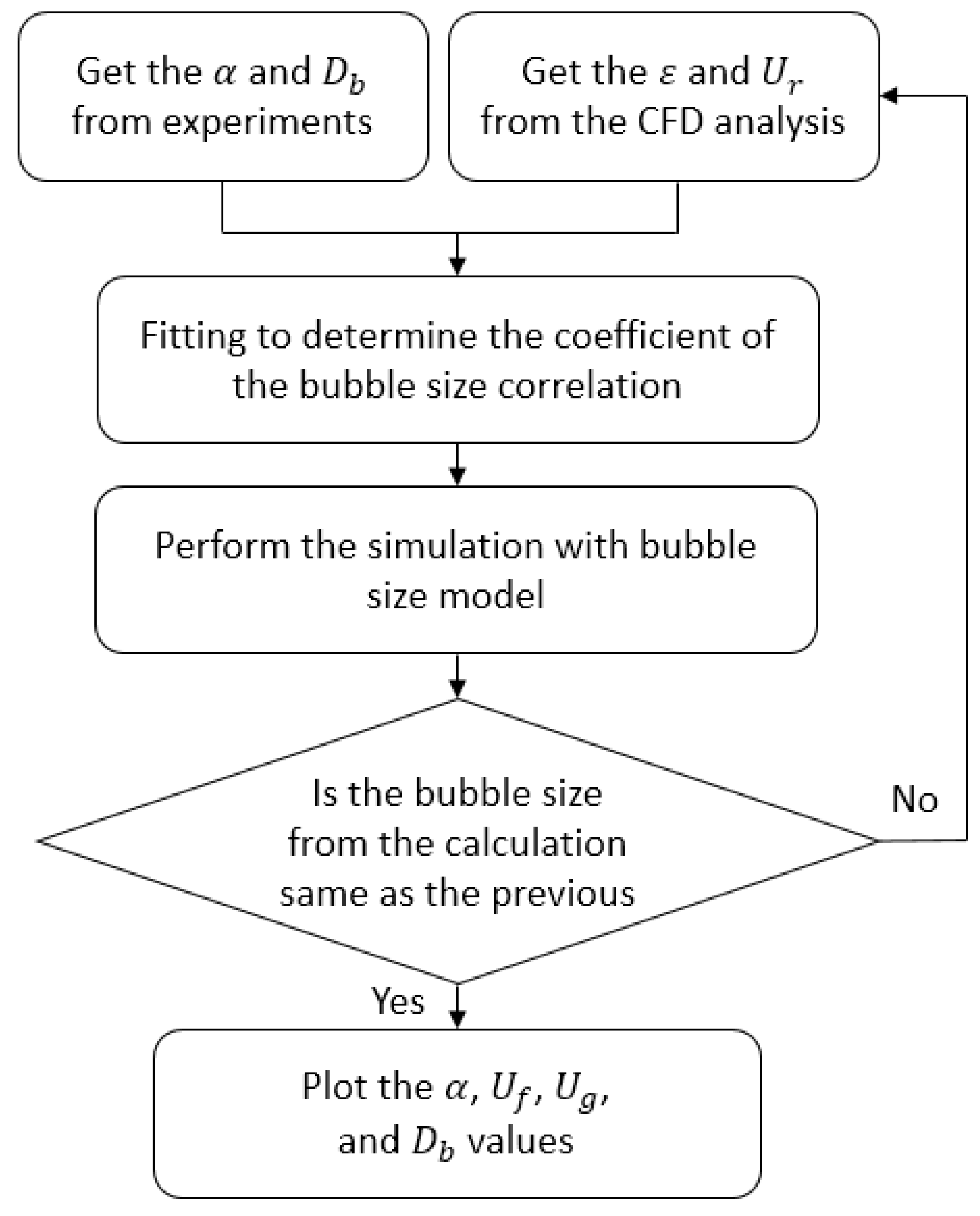
Finally, considering the dependency of variables, we proposed the following bubble size correlation for a bubbly flow under a steady-state fully developed condition by applying Equation (31) with the help of the iterative CFD calculation against the experimental database by following the procedure shown in Figure 2.
D b = 258.4 α 0.383 Re b 0.562 W e r 0.443 L o
The above correlation is a semi-theoretical correlation whose constant and exponents were obtained via multiple linear regression against the experiments by DEDALE [44], Hibiki et al. [45], and Kalkach-Navarro et al. [46]. The turbulent dissipation rate and relative velocity, which were not measured in the experiments, were obtained through CFD analysis.
Equation (32) satisfies the precondition that the bubble size should converge to zero when the void fraction tends toward zero. As the amount of void fraction increases, the random collision and the wake entrainment occur actively compared to the bubble breakup mechanism, and bubble size increases, and thus, the exponent of the void fraction is positive. As the turbulent dissipation rate and relative velocity increase, the turbulent impact for bubble breakup increases, and thus, bubble size decreases. Therefore, the exponent of the turbulent Reynolds numbers has a negative value.

5. Evaluation of Bubble Size Correlation with CFD Code

5.1. Experimental Database for the Simulation

We performed a CFD analysis of four forced convective air-water experiments under low-pressure conditions, as presented in Table 3, to evaluate the bubble size correlations. Table 4 presents the experimental conditions. All experiments were conducted in vertical pipes under the up-flow condition and obtained a radial distribution of local bubble parameters. The bubble shapes of the DEDALE [44], Hibiki [45], and Kalkach-Navarro [46] experiments are estimated as spherical, ellipsoid, and wobbling. However, we assumed a spherical bubble shape in the present study because the three experimental datasets and existing one group IATEs were obtained by applying a spherical bubble assumption. In this study, the forced convective air-water bubbly flow is considered to be a steady, adiabatic, and fully developed condition on the measuring plane [47].

5.2. Grid Sensitivity Test

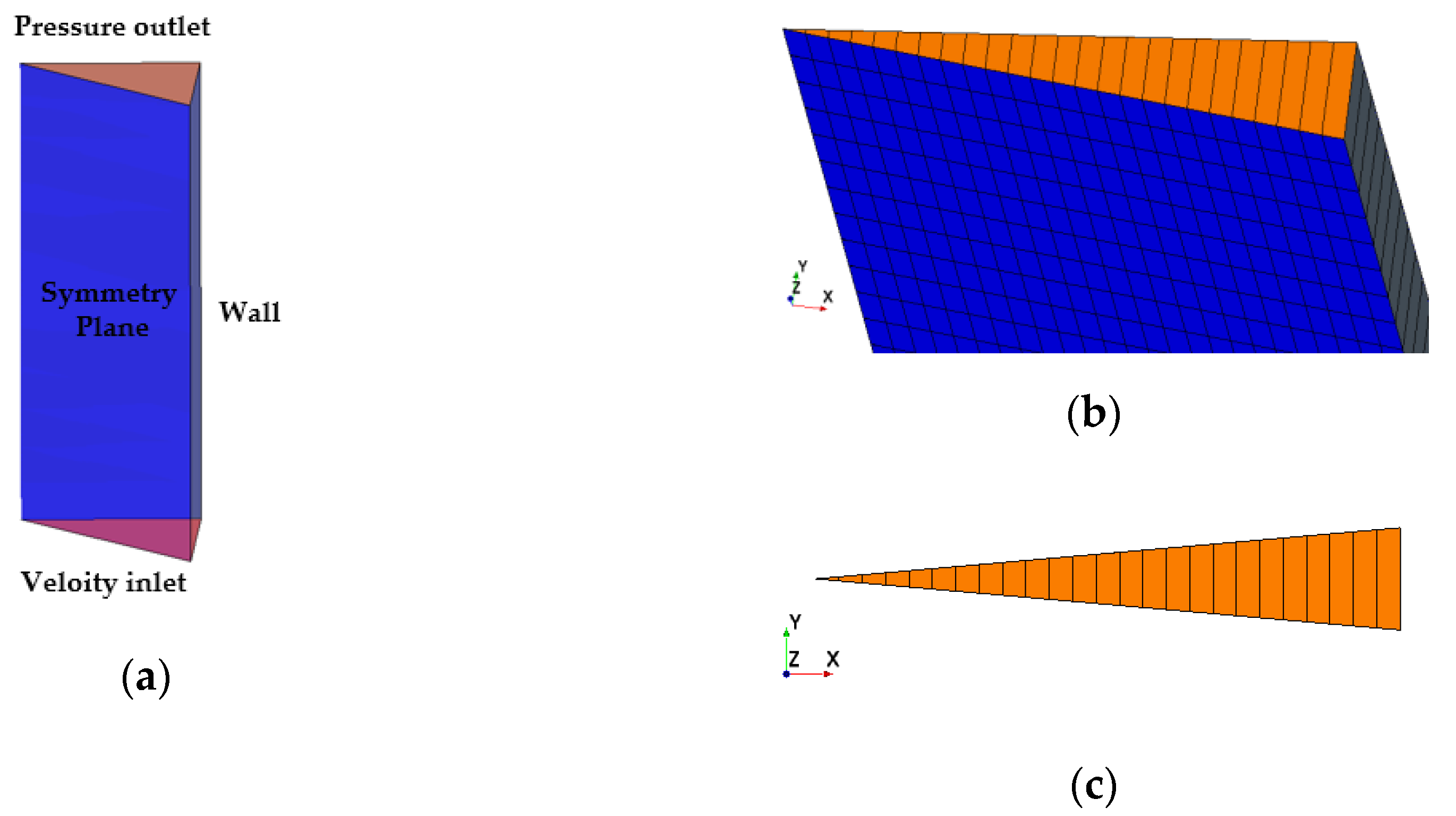
The fully developed forced convective bubbly flow in the vertical pipe was axisymmetric along the azimuthal direction; hence, we employed a quasi-2D cylindrical geometry for the simulation. This geometry is a narrow cylindrical sector with a central angle of 10°, which has symmetry boundary conditions on the side faces. The grid was divided into equal intervals along the axial direction. The flow domain and cross-sectional view of the grid are shown in Figure 3. The size in the axial direction was fixed at 5 mm, and the grid sensitivity test was conducted by changing the number of grids along the radial direction. The grid test was carried out with four meshes. Furthermore, we performed a grid geometry study with the full and half circular shapes for the simulation; however, there was no substantial difference in the calculation results. Here, the physical models introduced in Section 3 were used. Figure 4 compares the results obtained with different meshes in the Hibiki experiments. For the Hibiki experiment, 25 × 612 meshes revealed good independence on mesh and were, therefore, selected for the following calculation. A similar grid test was also performed for other experiments. The grids utilized in each of the calculations are summarized in Table 5.

5.3. Evaluation of the New Bubble Size Model

The proposed bubble size correlation was applied to the benchmark calculation of the CFD code against experiments. Figure 5, Figure 6, Figure 7 and Figure 8 show a comparison of the local two-phase flow parameters, such as the void fraction, bubble diameter, and phase velocities predicted with the proposed bubble size correlation and experimental data. Of the four experiments used to evaluate the correlation, the first three experiments listed in Table 5 were used to determine the coefficients of the correlation when developing the correlation; however, VAWL data were not used. The existing correlations investigated in Section 2 were also implemented in the CFD code and evaluated.
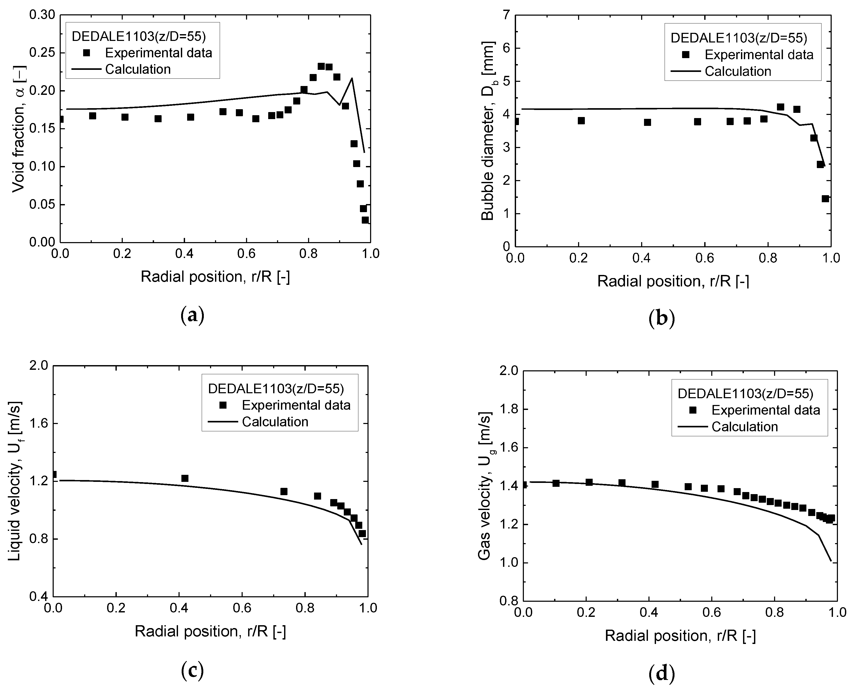
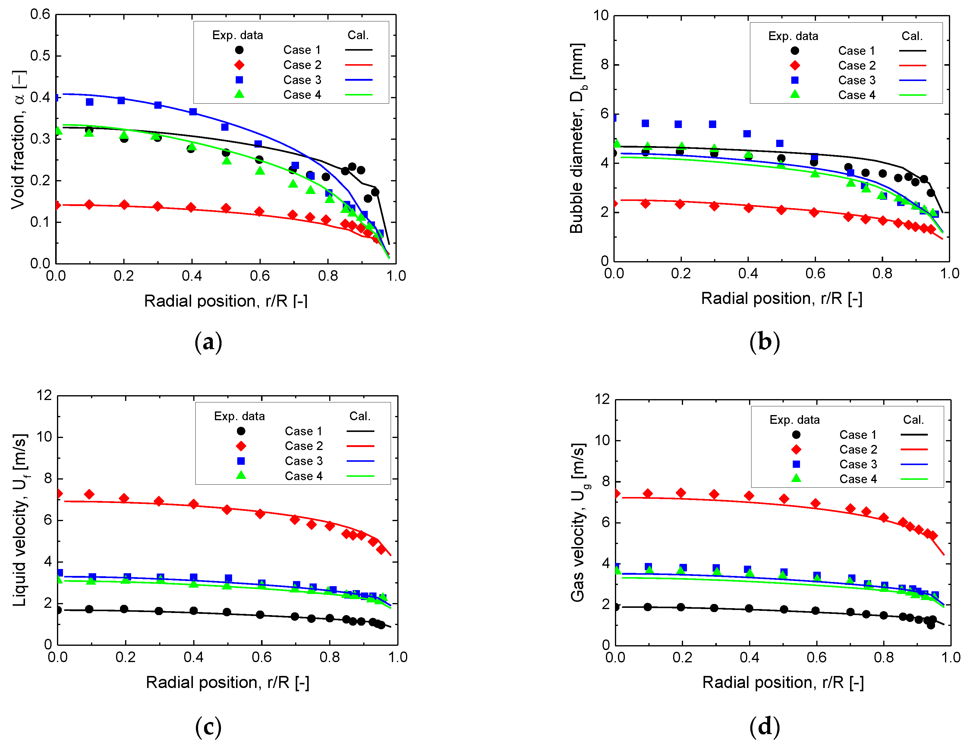
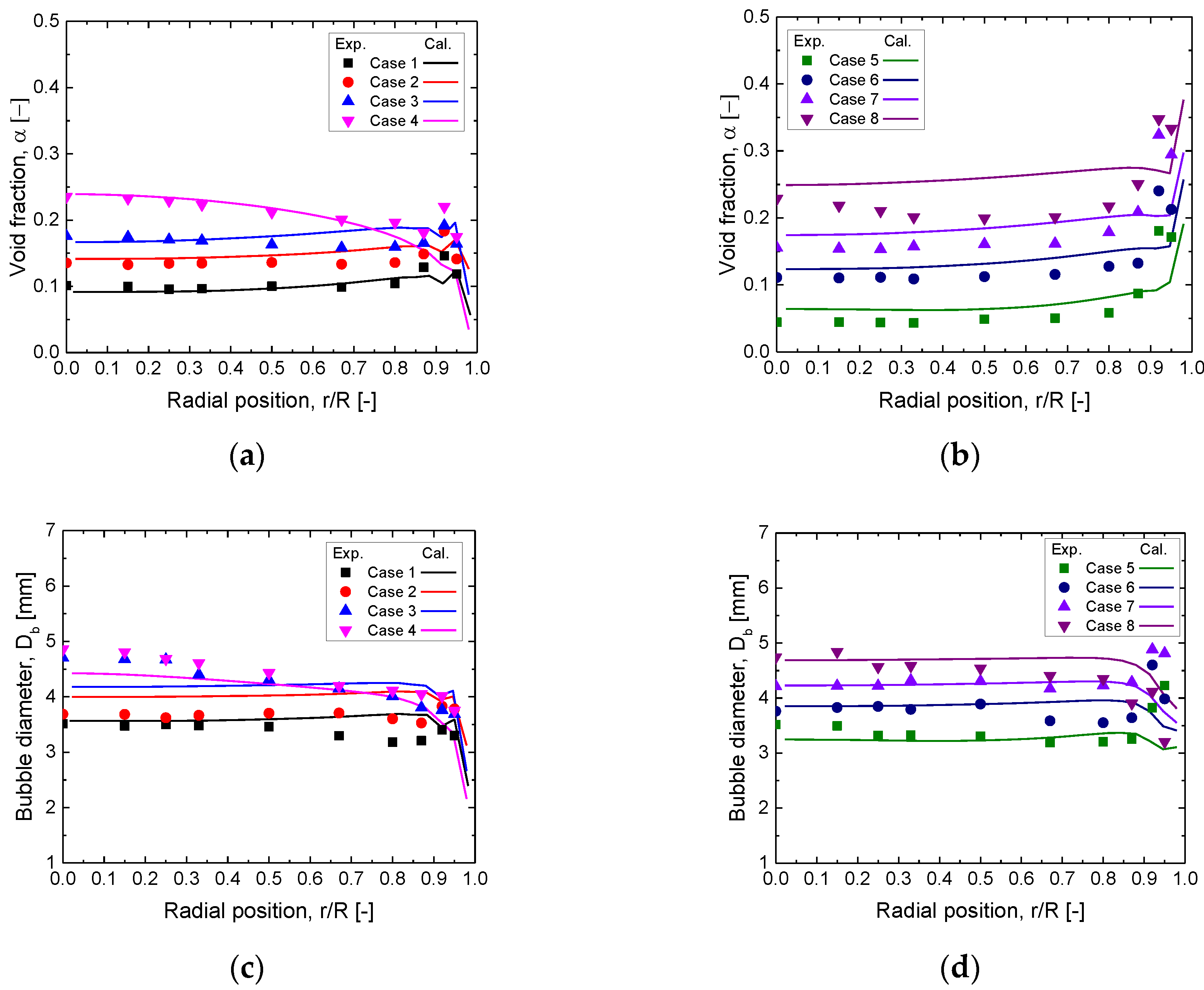
As illustrated in Figure 5, the numerical calculation result for the DEDALE experiment shows a flat void fraction distribution at the center of the pipe and a rapid increase in the vicinity of the wall with reasonable accuracy. Moreover, the bubble size and phase velocity are well predicted against the experimental data. For the four cases of Hibiki experiments, the peak void fraction in the channel center was well predicted, as depicted in Figure 6a. Additionally, the prediction of the phase velocities shows good agreement, as shown in Figure 6c,d. In Case 3 of the Hibiki experiment, the local void fraction for r/R < 0.7 exceeds 0.25 and, thus, the appearance of a slug bubble is expected [49]. Therfore, the relatively large bubbles at the center of the pipe could not be accurately predicted, even though their profiles closely followed the tendency of the bubble size, as shown in Figure 6b. For the Kalkach-Navarro experiment, the data on the velocity of the liquid and gas phase are not provided; only the void fraction and the bubble size are shown in Figure 7. Simulation results show that large bubbles, which appeared in the center in Cases 1–4, were not well predicted, similar to those in the Hibiki experiment. Furthermore, the increase in bubble size near the wall was not predicted in Cases 5–8. Thus, a second group bubble size model for large bubbles is required for better prediction. Nevertheless, the overall value and tendencies of the void fraction and bubble size were predicted with reasonable accuracy.
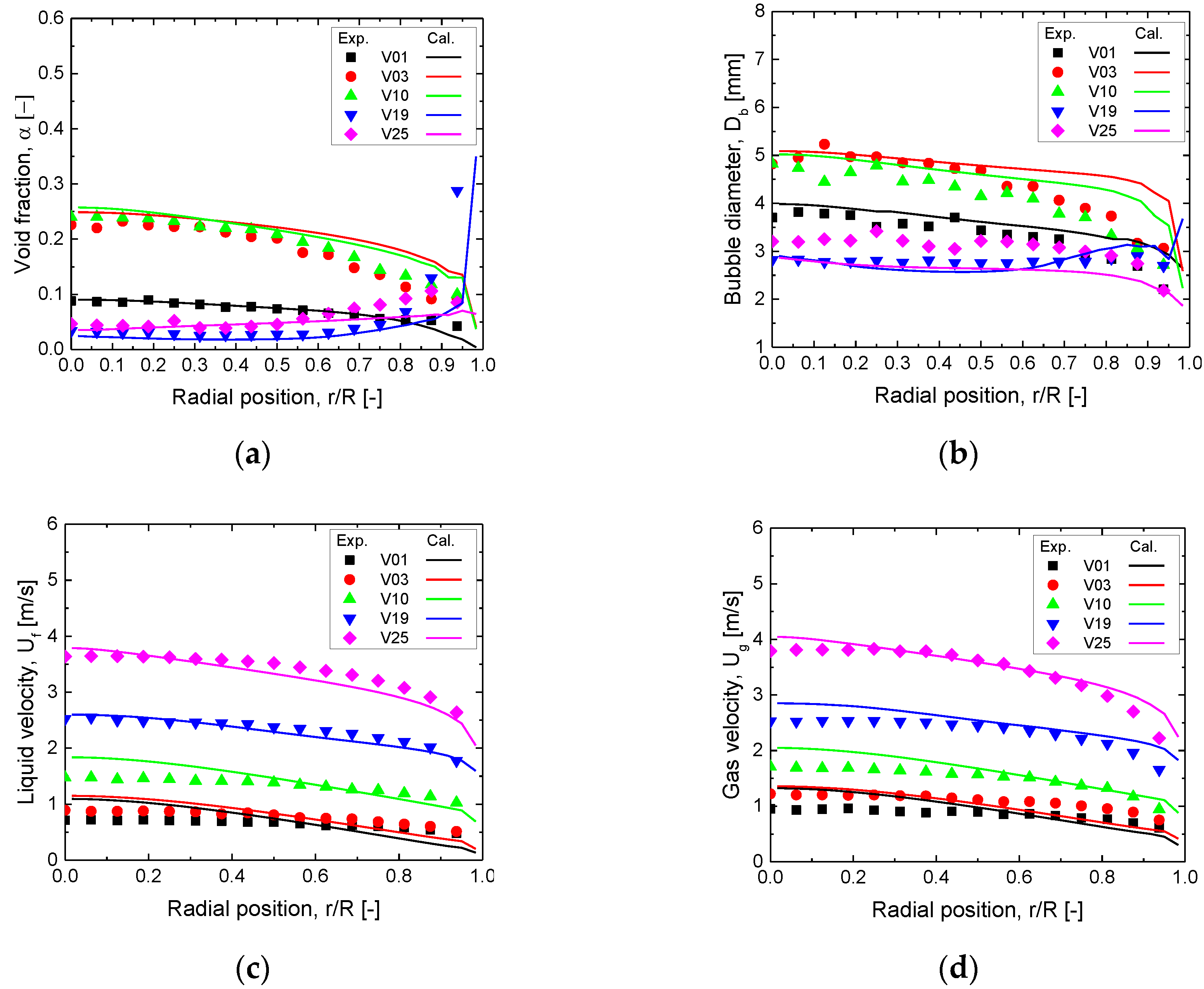
Finally, the new bubble size model was evaluated for the VAWL experiment, which was not used for determining the correlation coefficients. Figure 8 shows a comparison of the simulation results and experimental data for the local two-phase flow parameters, such as the void fraction, bubble diameter, and phase velocities. The VAWL data show both the core and wall peaks, where bubbles are concentrated at the center and near the wall, respectively, according to the experimental conditions. These phenomena were well predicted by the calculations. In V01 and V03, the void fraction in the nearby wall was overpredicted, and hence, bubble size was also overpredicted near the wall. The velocity of each phase was predicted to be slightly higher at the center. Nevertheless, the evaluation confirms that the proposed bubble size correlation predicts the overall value and tendencies of bubble size and phase velocity with reasonable accuracy.
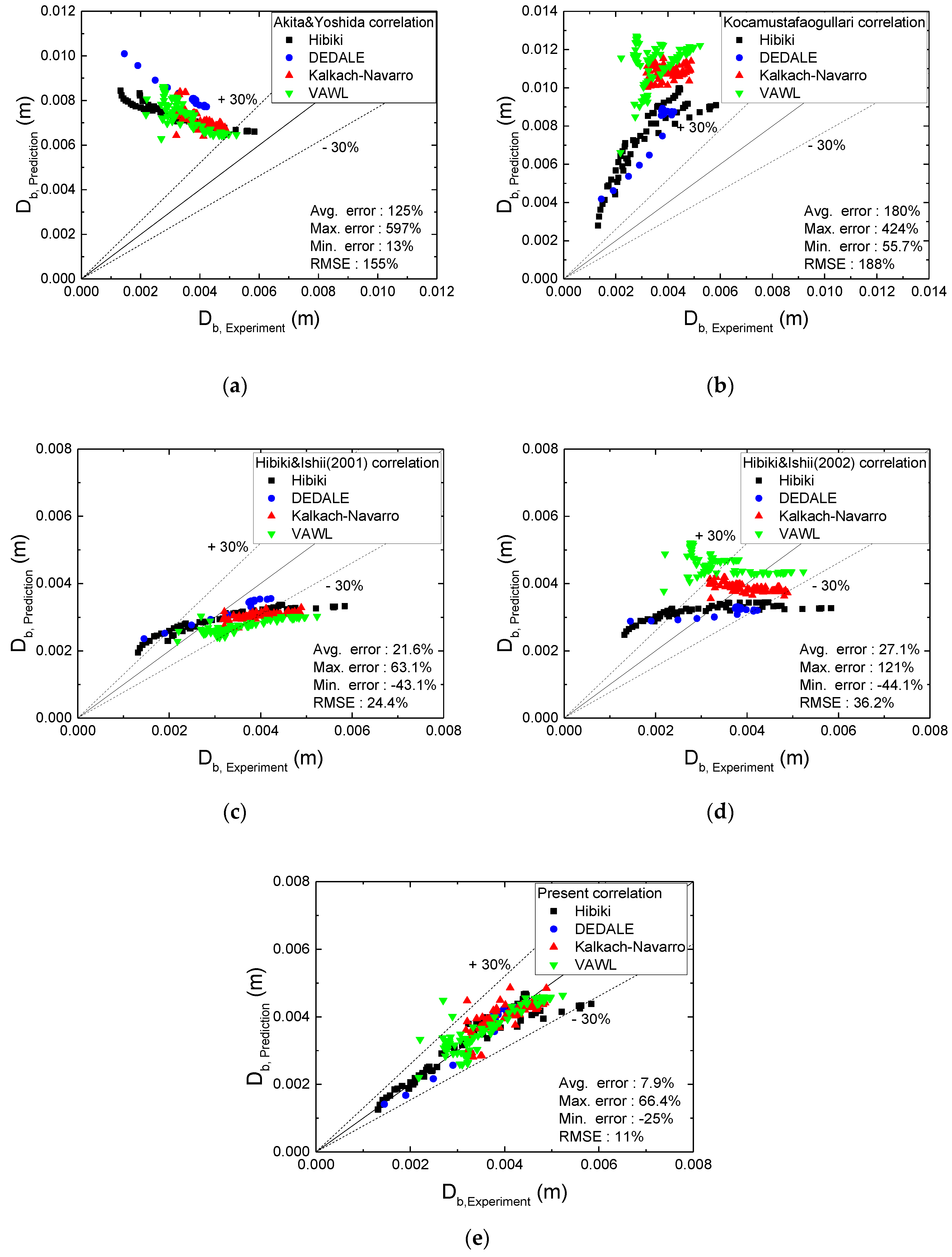
Figure 9 shows the performances of the existing bubble size correlations and the new bubble size correlation against the four experiments. The Akita and Yoshida correlation as well as the Kocamustafaogullari correlation significantly overpredicted the local bubble size and were unsuitable for the CFD code for a forced convective bubbly flow in a vertical pipe because the two correlations were developed under bubble column and horizontal tube conditions, respectively. Although the two Hibiki and Ishii correlations were developed using the average bubble size data in a flow channel, these correlations yielded acceptable predictions for the experimental data. The new bubble size correlation shows the best performance among all correlations. For quantification of the prediction accuracy of the existing and new correlations for the local bubble diameter, the average error and root-mean-square error (RMSE) are defined as follows:
E p r e d i c t i o n , D b = | D b , m e a s . D b , c a l c . | D b , m e a s . × 100
E R M S E , D b = 1 N i = 1 N ( D b , m e a s . D b , c a l c . ) 2 × 100
where N is the number of experimental datasets, Db, meas. is the local bubble size obtained through experiments, and Db, calc. is the calculated local bubble size with the correlation. The average error and RMSE are summarized in Table 6. Through the assessment of the new correlation with other correlations, the new correlation has an excellent agreement within an RMSE of ± 11% in the vertical adiabatic bubbly flow under the low pressure condition.

6. Conclusions

In this study, we developed a semi-theoretical bubble size correlation based on the bubble number density transport equation. The new correlation considers the random collision and wake entrainment for bubble coalescence and turbulent impact for bubble breakup, respectively. To determine the coefficient and exponent of the correlation, we utilized three different experimental databases obtained in a vertical adiabatic bubbly flow under low-pressure conditions.
To validate the performance of the new correlation, three-dimensional numerical simulations for four air-water experiments were carried out using commercial CFD code. The numerical results indicated that the correlation can be used to accurately predict air-water bubbly flow behavior. Through the assessment of the new correlation together with other existing one-dimensional correlations, the new correlation is in excellent agreement with the experimental data. The applicable condition of the new correlation covers forced convective bubbly flows, which are in the ranges of 38.1 mm ≤ hydraulic diameter (DH) ≤ 80 mm, 0.05 m/s ≤ superficial gas velocity (jg) ≤ 0.624 m/s, 0.5 m/s ≤ superficial liquid velocity (jf) ≤ 5 m/s, 1.32 mm ≤ bubble size (Db) ≤ 5.84 mm, 0.47 ≤ Eo ≤ 2.65, 171 ≤ Re ≤ 8785, and 1 bar ≤ absolute pressure (P) ≤ 3.5 bar.

Author Contributions

Conceptualization, B.Y.; Formal analysis, J.B.; Funding acquisition, B.Y.; Investigation, J.B. and H.K.; resources, D.E.; Methodology, J.B. and B.Y.; Project administration, B.Y.; Supervision, B.Y. and J.J.J.; Writing—original draft, J.B.; Writing—review and editing, J.B., J.J.J. and B.Y.; All authors have read and agreed to the published version of the manuscript.

Funding

This research was funded by Nuclear Research & Development Program of the National Research Foundation of Korea (NRF) grant funded by the Ministry of Science and ICT (MSIT) and by the Nuclear Safety Research Program through the Korea Foundation of Nuclear Safety (KOFONS) grant funded by Nuclear Safety and Security Commission (NSSC) of the Korean government (Grant code: NRF-2019M2D2A1A03056998, No.1903001).

Conflicts of Interest

The authors declare no conflict of interest.

References

  1. Wang, X.; Sun, X. Effects of Non-Uniform Inlet Boundary Conditions and Lift Force on Prediction of Phase Distribution in Upward Bubbly Flows with Fluent-IATE. Nucl. Eng. Des. 2011, 241, 2500–2507. [Google Scholar] [CrossRef]
  2. Ishii, M.; Kim, S.; Uhle, J. Interfacial area transport equation: Model development and benchmark experiments. Int. J. Heat Mass Transf. 2002, 45, 3111–3123. [Google Scholar] [CrossRef]
  3. Magnaudet, J.; Legendre, D. Some aspects of the lift force on a spherical bubble. Fascin. Fluid Dyn. A Symp. Honour Leen Van Wijng. 1998, 45, 441–461. [Google Scholar]
  4. Chahed, J.; Masbernat, L. Modeling Interfacial Interactions and Turbulence in the Near-Wall Region of a Vertical Bubbly Boundary Layer. J. Fluids Eng. 2020, 142. [Google Scholar] [CrossRef]
  5. Jin, D.; Xiong, J.; Cheng, X. Investigation on interphase force modeling for vertical and inclined upward adiabatic bubbly flow. Nucl. Eng. Des. 2019, 350, 43–57. [Google Scholar] [CrossRef]
  6. Lote, D.A.; Vinod, V.; Patwardhan, A.W. Computational fluid dynamics simulations of the air–water two-phase vertically upward bubbly flow in pipes. Ind. Eng. Chem. Res. 2018, 57, 10609–10627. [Google Scholar] [CrossRef]
  7. Kriebitzsch, S.; Rzehak, R. Baseline model for bubbly flows: Simulation of monodisperse flow in pipes of different diameters. Fluids 2016, 1, 29. [Google Scholar] [CrossRef]
  8. Yamoah, S.; Martínez-Cuenca, R.; Monrós, G.; Chiva, S.; Macián-Juan, R. Numerical Investigation of Models for Drag, Lift, Wall Lubrication and Turbulent Dispersion Forces for the Simulation of Gas-Liquid Two-Phase Flow. Chem. Eng. Res. Des. 2015, 98, 17–35. [Google Scholar] [CrossRef]
  9. Rzehak, R.; Krepper, E. Bubble-induced turbulence: Comparison of CFD models. Nucl. Eng. Des. 2013, 258, 57–65. [Google Scholar] [CrossRef]
  10. Frank, T.; Zwart, P.J.; Krepper, E.; Prasser, H.M.; Lucas, D. Validation of CFD models for mono-and polydisperse air–water two-phase flows in pipes. Nucl. Eng. Des. 2008, 238, 647–659. [Google Scholar] [CrossRef]
  11. Gemello, L.; Plais, C.; Augier, F.; Marchisio, D.L. Population balance modelling of bubble columns under the heterogeneous flow regime. Chem. Eng. J. 2019, 372, 590–604. [Google Scholar] [CrossRef]
  12. Marfaing, O.; Guingo, M.; Laviéville, J.; Bois, G.; Méchitoua, N.; Mérigoux, N.; Mimouni, S. An Analytical Relation for the Void Fraction Distribution in a Fully Developed Bubbly Flow in a Vertical Pipe. Chem. Eng. Sci. 2016, 152, 579–585. [Google Scholar] [CrossRef] [Green Version]
  13. Wu, Q.; Kim, S.; Ishii, M.; Beus, S.G. One-group interfacial area transport in vertical bubbly flow. Int. J. Heat Mass Transf. 1998, 41, 1103–1112. [Google Scholar] [CrossRef]
  14. Hibiki, T.; Ishii, M. Interfacial area transport equations for gas-liquid flow. J. Comput. Multiph. Flows 2009, 1, 1–22. [Google Scholar] [CrossRef] [Green Version]
  15. Yao, W.; Morel, C. Volumetric interfacial area prediction in upward bubbly two-phase flow. Int. J. Heat Mass Transf. 2004, 47, 307–328. [Google Scholar] [CrossRef]
  16. Yeoh, G.H.; Tu, J.Y. A unified model considering force balances for departing vapour bubbles and population balance in subcooled boiling flow. Nucl. Eng. Des. 2005, 235, 1251–1265. [Google Scholar] [CrossRef]
  17. Lo, S.; Zhang, D. Modelling of break-up and coalescence in bubbly two-phase flows. J. Comput. Multiph. Flows 2009, 1, 23–38. [Google Scholar] [CrossRef] [Green Version]
  18. Yun, B.J.; Splawski, A.; Lo, S.; Song, C.H. Prediction of a subcooled boiling flow with advanced two-phase flow models. Nucl. Eng. Des. 2012, 253, 351–359. [Google Scholar] [CrossRef]
  19. Duan, X.Y.; Cheung, S.C.P.; Yeoh, G.H.; Tu, J.Y.; Krepper, E.; Lucas, D. Gas–liquid flows in medium and large vertical pipes. Chem. Eng. Sci. 2011, 66, 872–883. [Google Scholar] [CrossRef]
  20. Akita, K.; Yoshida, F. Bubble size, interfacial area, and liquid-phase mass transfer coefficient in bubble columns. Ind. Eng. Chem. Process Des. Dev. 1974, 13, 84–91. [Google Scholar] [CrossRef]
  21. Kocamustafaogullari, G.; Huang, W.D.; Razi, J. Measurement and modeling of average void fraction, bubble size and interfacial area. Nucl. Eng. Des. 1994, 148, 437–453. [Google Scholar] [CrossRef]
  22. Hibiki, T.; Ishii, M. Interfacial area concentration in steady fully-developed bubbly flow. Int. J. Heat Mass Transf. 2001, 44, 3443–3461. [Google Scholar] [CrossRef]
  23. Hibiki, T.; Ishii, M. Interfacial area concentration of bubbly flow systems. Chem. Eng. Sci. 2002, 57, 3967–3977. [Google Scholar] [CrossRef]
  24. Ozar, B.; Dixit, A.; Chen, S.W.; Hibiki, T.; Ishii, M. Interfacial area concentration in gas–liquid bubbly to churn-turbulent flow regime. Int. J. Heat Fluid Flow 2012, 38, 168–179. [Google Scholar] [CrossRef]
  25. Shen, X.; Hibiki, T. Interfacial area concentration in gas–liquid bubbly to churn flow regimes in large diameter pipes. Int. J. Heat Fluid Flow 2015, 54, 107–118. [Google Scholar] [CrossRef]
  26. Schlegel, J.P.; Hibiki, T. A correlation for interfacial area concentration in high void fraction flows in large diameter channels. Chem. Eng. Sci. 2015, 131, 172–186. [Google Scholar] [CrossRef]
  27. Fu, X.Y.; Ishii, M. Two-group interfacial area transport in vertical air–water flow: I. Mechanistic model. Nucl. Eng. Des. 2003, 219, 143–168. [Google Scholar] [CrossRef]
  28. Hinze, J.O. Fundamentals of the hydrodynamic mechanism of splitting in dispersion processes. Aiche J. 1955, 1, 289–295. [Google Scholar] [CrossRef]
  29. Jones, W.P.; Launder, B.E. The Prediction of Laminarization with a Two-Equation Model of Turbulence. Int. J. Heat Mass Tranf. 1972, 15, 301–314. [Google Scholar] [CrossRef]
  30. Launder, B.E.; Sharma, B.I. Application of the Energy Dissipation Model of Turbulence to the Calculation of Flow Near a Spinning Disc. Lett. Heat Mass Transf. 1974, 1, 131–138. [Google Scholar] [CrossRef]
  31. Siemens. Star-CCM+ User Guide. 13.06.012; Siemens: Munich, Germany, 2016. [Google Scholar]
  32. Tomiyama, A.; Kataoka, I.; Zun, I.; Sakaguchi, T. Drag coefficients of single bubbles under normal and micro gravity conditions. JSME Int. J. Ser. B Fluids Therm. Eng. 1998, 41, 472–479. [Google Scholar] [CrossRef]
  33. Auton, T.R.; Hunt, J.C.R.; Prud’Homme, M. The force exerted on a body in inviscid unsteady non-uniform rotational flow. J. Fluid Mech. 1988, 197, 241–257. [Google Scholar] [CrossRef]
  34. Lahey Jr, R.T.; De Bertodano, M.L.; Jones, O.C., Jr. Phase distribution in complex geometry conduits. Nucl. Eng. Des. 1993, 141, 177–201. [Google Scholar] [CrossRef] [Green Version]
  35. Troshko, A.A.; Hassan, Y.A. A two-equation turbulence model of turbulent bubbly flows. Int. J. Multiph. Flow 2001, 27, 1965–2000. [Google Scholar] [CrossRef]
  36. Antal, S.P.; Lahey, R.T., Jr.; Flaherty, J.E. Analysis of phase distribution in fully developed laminar bubbly two-phase flow. Int. J. Multiph. Flow 1991, 17, 635–652. [Google Scholar] [CrossRef]
  37. Morel, C. Turbulence Modeling and First Numerical Simulations in Turbulent Two-Phase Flows; Technical Report; CEA: Grenoble, France, 1997. [Google Scholar]
  38. Politano, M.; Carrica, P.; Converti, J. A model for turbulent polydisperse two-phase flow in vertical channels. Int. J. Multiph. Flow 2003, 29, 1153. [Google Scholar] [CrossRef]
  39. Sato, Y.; Sadatomi, M.; Sekoguchi, K. Momentum and heat transfer in two-phase bubble flow—I. Theory. Int. J. Multiph. Flow 1981, 7, 167–177. [Google Scholar] [CrossRef]
  40. Lopez de Bertodano, M.; Lahey, R.T., Jr.; Jones, O.C. Development of a k-ε model for bubbly two-phase flow. J. Fluid Eng. 1994, 116, 128–134. [Google Scholar] [CrossRef]
  41. Behzadi, A.; Issa, R.I.; Rusche, H. Modelling of dispersed bubble and droplet flow at high phase fractions. Chem. Eng. Sci. 2004, 59, 759–770. [Google Scholar] [CrossRef]
  42. Hibiki, T.; Ishii, M. One-group interfacial area transport of bubbly flows in vertical round tubes. Int. J. Heat Mass Transf. 2000, 43, 2711–2726. [Google Scholar] [CrossRef]
  43. Hibiki, T.; Takamasa, T.; Ishii, M. Interfacial area transport of bubbly flow in a small diameter pipe. J. Nucl. Sci. Technol. 2001, 38, 614–620. [Google Scholar] [CrossRef]
  44. Michta, E. Modeling of subcooled nucleate boiling with OpenFOAM. Master’s Thesis, Division of Nuclear Reactor Technology Royal Institute of Technology, Stockholm, Sweden, February 2011. [Google Scholar]
  45. Hibiki, T.; Ishii, M.; Xiao, Z. Axial interfacial area transport of vertical bubbly flows. Int. J. Heat Mass Transf. 2001, 44, 1869–1888. [Google Scholar] [CrossRef]
  46. Kalkach-Navarro, S.; Lahey, R.T., Jr.; Drew, D.A.; Meyder, R. Interfacial area density, mean radius and number density measurements in bubbly two-phase flow. Nucl. Eng. Des. 1993, 142, 341–351. [Google Scholar] [CrossRef]
  47. Islam, A.A.; Bergstrom, D.J. Modelling bubble induced turbulence for gas-liquid bubbly flow in a vertical pipe. Chem. Eng. Sci. 2019, 197, 159–171. [Google Scholar] [CrossRef]
  48. Song, C.H. Integral Cooling Performance Tests for Nuclear Power Plants and Development of Advanced Safety Analysis Technology (Thermal-Hydraulic Experiment for Advanced Physical Model Development); KAERI/RR-3437/2011; KAERI: Seul, Korea, 2011. [Google Scholar]
  49. Taitel, Y.; Bornea, D.; Dukler, A.E. Modelling flow pattern transitions for steady upward gas-liquid flow in vertical tubes. AIChE J. 1980, 26, 345–354. [Google Scholar] [CrossRef]
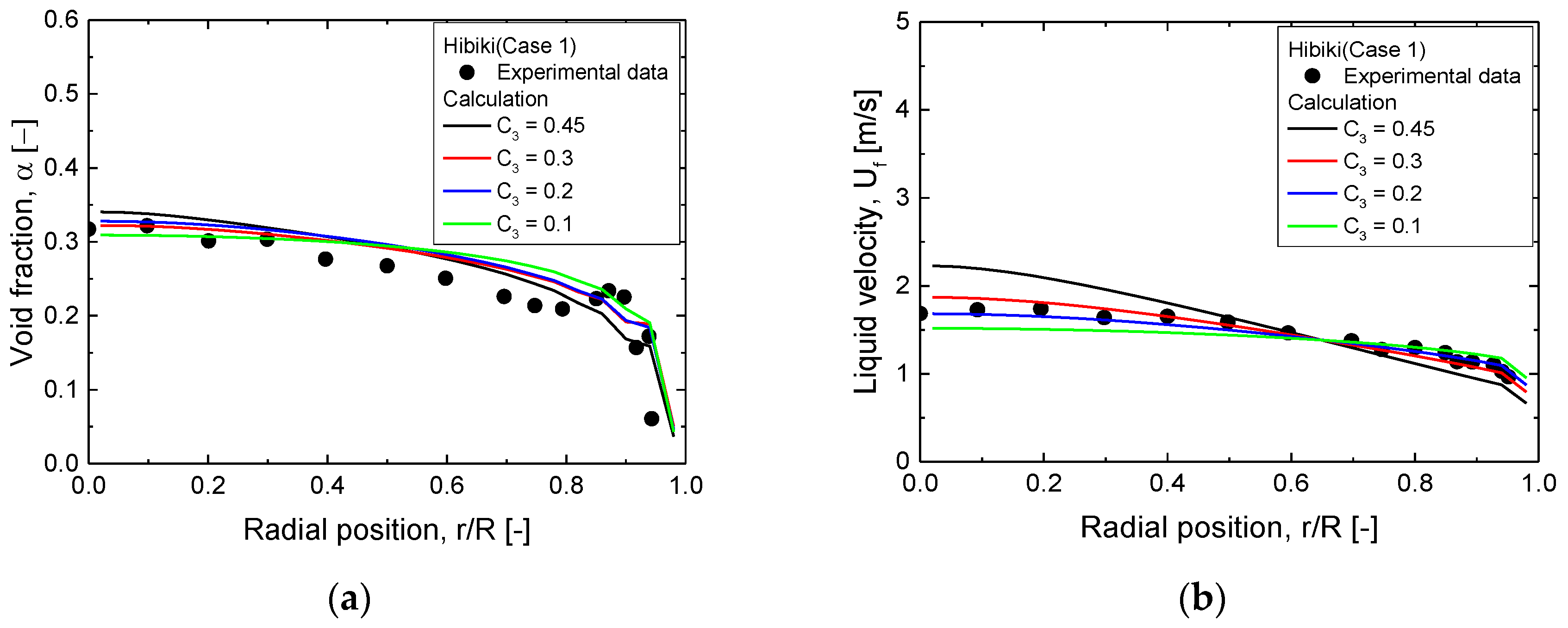
Figure 1. Prediction of radial distribution of (a) void fraction, and (b) liquid velocity by the different coefficients of Troshko and Hassan’s BIT model.
Applsci 10 05443 g001
Figure 2. Iterative calculation procedure for the development of the bubble size model.
Applsci 10 05443 g002
Figure 3. (a) Flow domain with boundary conditions, (b) grid near the outlet, and (c) cross-section of the grid.
Applsci 10 05443 g003
Figure 4. Results of grid sensitivity study for the Hibiki experiment.
Applsci 10 05443 g004
Figure 5. Comparison of the predicted two-phase parameters with the DEDALE experiment: (a) void fraction, (b) bubble diameter, (c) liquid velocity, and (d) gas velocity.
Applsci 10 05443 g005
Figure 6. Comparison of the predicted two-phase parameters with the Hibiki experiment: (a) void fraction, (b) bubble diameter, (c) liquid velocity, and (d) gas velocity.
Applsci 10 05443 g006
Figure 7. Comparison of the predicted two-phase parameters with the Kalkach-Navarro experiment: (a) void fraction (Cases 1–4), (b) void fraction (Cases 5–8), (c) bubble diameter (Cases 1–4), and (d) bubble diameter (Cases 5–8).
Applsci 10 05443 g007
Figure 8. Comparison of the predicted two-phase parameters with the VAWL experiment: (a) void fraction, (b) bubble diameter, (c) liquid velocity, and (d) gas velocity.
Applsci 10 05443 g008
Figure 9. Comparison of the predicted local bubble size and experimental data with (a) Akita and Yoshida, (b) Kocamustafaogullari, (c) Hibiki and Ishii (2001), (d) Hibiki and Ishii (2002), and (e) the present correlation.
Applsci 10 05443 g009
Table 1. Existing one group bubble size correlations for the gas-liquid system.
InvestigatorsBubble Size CorrelationApplication Conditions
Flow ConditionChannel Geometryjg (m/s)jf (m/s)
Akita and Yoshida [20] D b = 18 ν f 0.2 α 0.13 g 0.6 D H 0.3 ( σ ρ f ) 0.5 upward bubble columnsvertical square channel0.0007–0.0730
Kocamustafaogullari et al. [21] D b = 0.707 D H 0.44 α 0.22 ε 0.22 ( σ ρ f ) 0.33 cocurrent bubbly flowhorizontal pipe0.21–1.343.74–6.59
Hibiki and Ishii [22] D b = 12 α 0.153 ν f 0.212 ε 0.0707 D H 0.283 ( σ g Δ ρ ) 0.5 adiabatic, diabatic bubbly flowvertical pipe, horizontal pipe, annulus, bundle0.0029–4.870.261–6.55
Hibiki and Ishii [23] D b = 1.99 D H 0.335 ν f 0.239 ε 0.797 ( g Δ ρ σ ) 0.346 adiabatic, diabatic bubbly flow, bubble columnsvertical pipe, horizontal pipe, annulus, bundle0.0007–4.870–6.55
Table 2. Models for bubble breakup and coalescence.
MechanismModelReference
Turbulent impact ϕ T I = γ B α ( 1 α ) ε 1 / 3 D b 11 / 3 ( α max α ) exp ( K B σ ρ c D b 5 / 3 ε 2 / 3 ) Hibiki and Ishii [42]
Random collision ϕ R C = γ C α 2 ε 1 / 3 D b 11 / 3 ( α max α ) exp ( K C ρ c 1 / 2 D b 5 / 6 ε 1 / 3 σ 1 / 2 ) Hibiki and Ishii [42]
Wake entrainment ϕ W E = γ W E ( g Δ ρ ( 1 α ) ρ c ) 1 / 3 α 2 U r 2 / 3 D b 11 / 3 exp ( K C ρ c 1 / 2 D b 5 / 6 ε 1 / 3 σ 1 / 2 ) Hibiki et al. [43]
Table 3. Air-water bubbly flow experiments used to evaluate the bubble size correlation.
ExperimentInner Diameter (mm)Height (m)Measurement Location (z/D)
DEDALE [44]38.1655
Hibiki [45]50.83.0653.5
Kalkach-Navarro [46]603.550
VAWL [48]801042.2
Table 4. Experimental conditions of each experiment used to simulation.
ExperimentSuperficial Gas Velocity (m/s)Superficial Liquid Velocity (m/s)Void Fraction (−)Absolute Pressure at the Outlet (Bar)
DEDALE11030.18510.8770.1521.0
HibikiCase 10.3210.9860.2311.0
Case 20.51850.106
Case 30.6242.010.228
Case 40.4712.010.183
Kalkach-NavarroCase 10.0810.50.1093.5
Case 20.1140.50.142
Case 30.1350.50.169
Case 40.1480.50.211
Case 50.11.00.077
Case 60.1911.00.138
Case 70.271.00.195
Case 80.41.00.241
VAWLV010.050.50.0631.0
V030.160.50.1611.0
V100.2710.1631.0
V190.1220.0732.0
V250.172.850.0631.0
Table 5. Grids used in the benchmark calculation of each experiment.
ExperimentsRadialAxial
DEDALE251200
Hibiki25612
Kalkach-Navarro30700
VAWL301000
Table 6. Average error and RMSE of the bubble size correlation for each experiment.
Bubble Size CorrelationAverage ErrorRMSE
Akita and Yoshida125%155%
Kocamustafaogullari180%188%
Hibiki and Ishii (2001)21.6%24.4%
Hibiki and Ishii (2002)27.1%36.2%
Present7.9%11%