Local Phase-Amplitude Joint Correction for Free Surface Velocity of Hopkinson Pressure Bar

Featured Application

Reflected near-field blast pressure measurement.

Abstract

The Hopkinson pressure bar is widely used to measure the reflected pressure of blast waves over a short distance. However, dispersion effects will occur when the elastic stress waves propagate in the pressure bar due to lateral inertia, and there will be errors between the signals obtained from the sensors and the actual loading. For the free surface velocity measured in our system, we developed a local phase-amplitude joint correction method to convert the measured velocity into the average reflected pressure of a shock wave at the impact end of the bar, considering factors such as propagation modes of the elastic wave, the frequency components’ time of arrival, velocity variation over the bar axis, and the stress–velocity relationship. Firstly, the Pochhammer–Chree frequency equation is calculated numerically, and the first to fourth orders of phase velocity, group velocity, normalized frequency, and propagation time curves of elastic wave propagation in 35CrMnSiA steel are obtained. Secondly, the phase and amplitude correction formulas for calculating average reflected pressure from center velocity are derived based on the propagation mode of the axial elastic wave in the pressure bar by analyzing the time-frequency combined spectrum obtained by short-time Fourier transform. Thirdly, a local phase-amplitude joint correction algorithm based on propagation mode is proposed in detail. The experimental tests and data analyses are carried out for eight sets of pressure bar. The results show that this method can identify the propagation mode of elastic waves in the bar intuitively and clearly. The first three orders of propagation modes are stimulated in the bar 04, while only the first order of propagation is stimulated in the other eight bars. The local phase-amplitude joint correction algorithm can avoid correcting the component of the non-axial elastic wave. The rising edge of the average stress curve on the impact surface of bar 01 and bar 04 is corrected from 4.13 μs and 4.09 μs to 2.70 μs, respectively.

1. Introduction

The Hopkinson pressure bar has been the primary means of recording expected high magnitude, short duration, initial loading for over one hundred years, since 1914 [1]. The technology is still widely used in the research fields of explosion [2,3] and shock wave structural interaction [4]. As a sensitive element, the slender cylindrical bar is mainly optimized in material and size, while the measuring element is developed from detachable end-pieces [1], capacitance [5], and a strain gauge [6] attached to photonic doppler velocimetry (PDV) [7].

The main problem that has puzzled the measurement scientists is that the axial elastic stress wave is dispersed due to the lateral inertia effect, which leads to inconsistency between the signal obtained by the measuring element and the actual load on the front end of the pressure bar. The theoretical basis of most dispersion analysis and correction methods is the analytical solution of axisymmetric load in an infinite isotropic elastic circular bar, independently proposed by Pochhammer [8] and Chree [9], which is generally called the P-C frequency equation. In 1941, Bancroft [10] used a numerical calculation method to solve the P-C frequency equation and obtained the first-order phase velocity curve and displacement along the radius of the section of the axial elastic stress wave in the cylindrical bar under different Poisson’s ratios. In 1948, Davies [5] experimentally verified the solution of the P-C equation and found that the group velocity of the high-frequency component of the stress pulse in the basic propagation mode is lower than the low-frequency component, so the high-frequency oscillation follows the main pulse. In 1978, Yew [11] used the fast Fourier transform method to analyze the strain signals at two measuring points on the pressure bar, and the phase velocity of each frequency component of the axial longitudinal wave obtained was consistent with the theoretical value of the first-order propagation mode of the P-C equation. These studies prove that the finite length pressure bar can still be studied based on P-C theory in practical applications.

Gorham [12] and Follansbee and Frantz [13] independently calculated phase shifts from the first mode of the Pochhammer–Chree dispersion relation and the sensor’s distance from the pressure end. The incident signal is reconstructed from the frequency components, undispersed by the phase shifts. This frequency domain phase-shift method is already commonly employed in practical pressure bar work (e.g., Gong [14], Lifshitz [15], Zhao [16]). In 1995, Lee [17] constructed a group velocity curve from the Gaussian-windowed Fourier transform of the measured signal. The frequency components of the signal are shifted according to the mode with the dominant group velocity. Tyas [18,19,20] improved the dispersion correction method by the application of additional correction factors to the amplitude of the Fourier components, derived from the Pochhammer–Chree results for axial strain variation over the bar radius and stress–strain relationship. Rigby [21] presents a detailed review of the current status of Hopkinson pressure bar data analysis.

For the free surface velocity measured in our system, we developed a local phase-amplitude joint correction method considering factors such as propagation mode of the elastic wave, frequency components’ time of arrival, velocity variation over the bar axis, and the stress–velocity relation. This method has the capability of identifying the propagation mode and correcting multi-mode dispersion except for the non-axial elastic wave.

2. Principle

2.1. Propagation Characteristics of Elastic Stress Wave in Cylindrical Bar

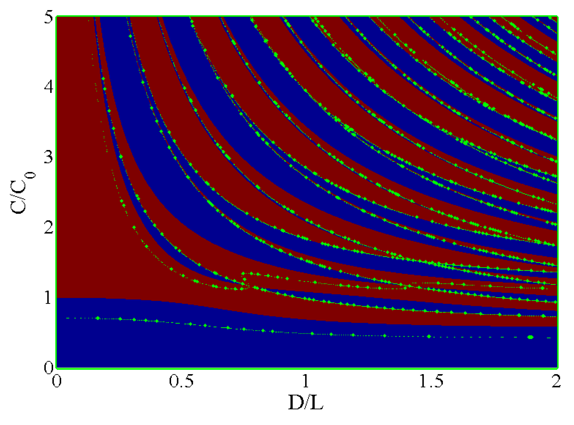
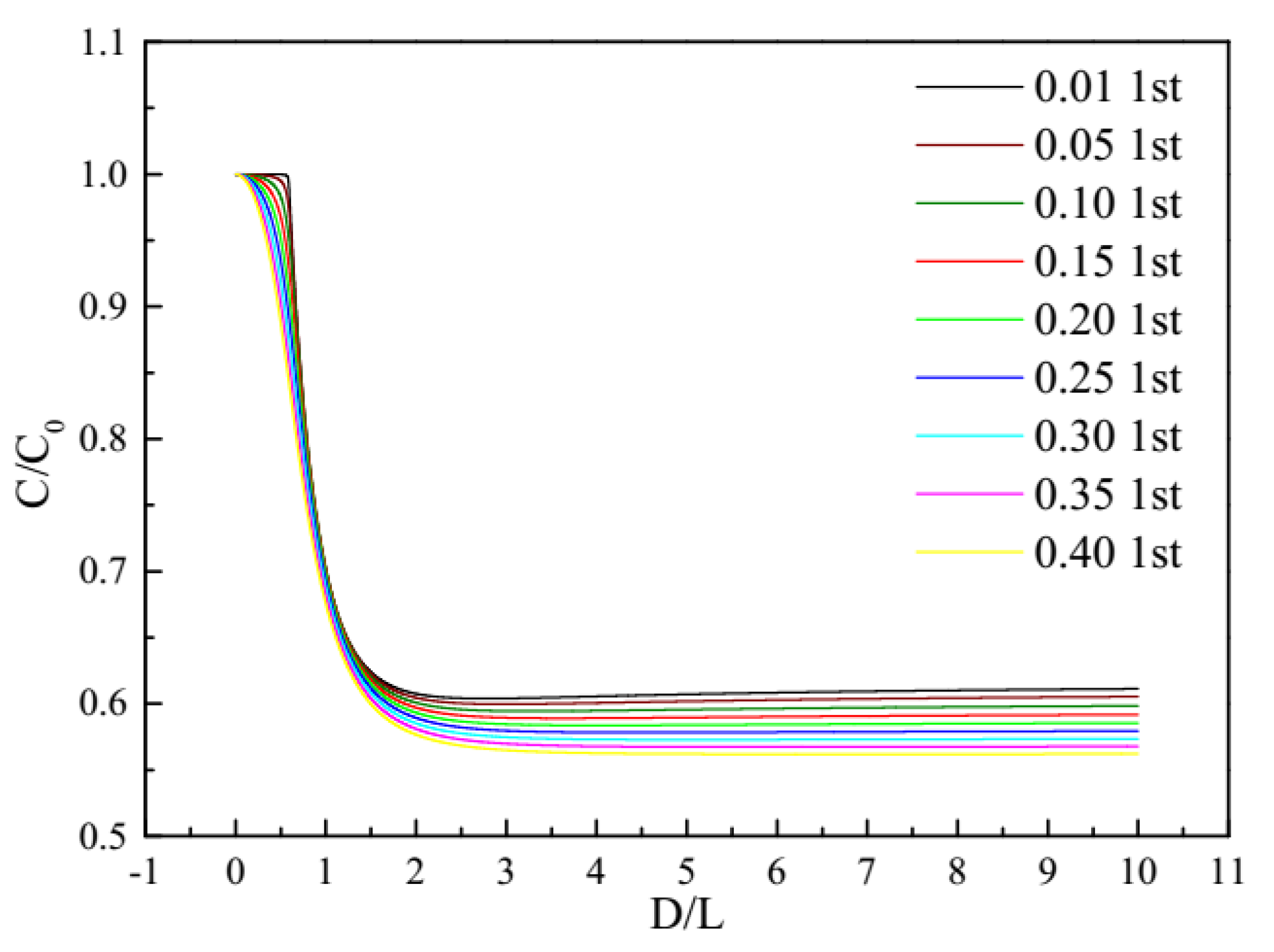
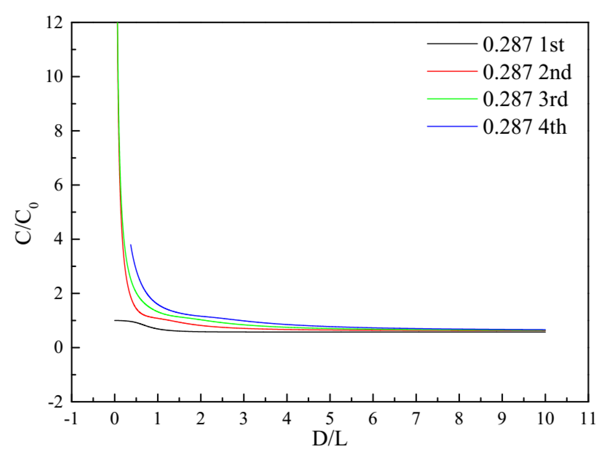
2.1.1. Phase Velocity Curve in Bar

The material of the pressure bar is assumed to be isotropic, homogeneous, linear elastic, and undamped. The front end face of the pressure bar is the pressure bearing surface, which keeps a certain distance from the explosion center so that the pressure peak value is lower than the yield strength, which ensures that the elastic stress wave propagates in the bar. Bancroft simplified the P-C frequency equation into:

$${\left(x-1\right)}^2\phi \left(ha\right)-\left(\beta x-1\right)\left[x-\phi \left(ka\right)\right]=0$$

(1)

where the definition of each parameter is shown in

Table 1. Definition of elastic longitudinal stress wave parameters in the bar.

Parameter	Definition
$C$	phase velocity
$C_g$	group velocity
$C_0$	longitudinal wave velocity
$L$	wavelength
$\gamma =2\pi /L$	wave number
$f$	frequency
$\omega =2\pi f$	angular frequency
$D$	diameter of pressure bar
$a=D/2$	radius of pressure bar
$\sigma$	Poisson’s ratio
$\beta =\left(1-2\sigma \right)/\left(1-\sigma \right)$	intermediate parameters
$x=\left(1+\sigma \right){\left(C/C_0\right)}^2$	intermediate parameters
$E$	Young’s modulus
$\mu =E/2\left(1+\sigma \right)$	modulus of rigidity
$h=\gamma {\left(\beta x-1\right)}^{0.5}$	intermediate parameters
$k=\gamma {\left(2x-1\right)}^{0.5}$	intermediate parameters
$\phi \left(y\right)=y{J}_0\left(y\right)/J_1\left(y\right)$	composite function based on the Bessel function of the first kind

. The formula is a function of $x$, $\beta$, and $\gamma a$, in which $\beta$ is related to Poisson’s ratio of material. When the material is selected, its value has been determined. $x$ is the relationship between the propagation phase velocity of the elastic longitudinal wave at a certain wavelength and the elementary theoretical wave velocity, and $\gamma a$ is related to the ratio of bar radius to wavelength. Therefore, formula (1) actually gives the relationship between wavelength and wave velocity.

Because of the properties of the Bessel function, Formula (1) has infinite sets of solutions, and it is difficult to obtain its analytical solution. Take $C/C_0$ and $D/L$ as values in a certain range, and then calculate the value of the function on the left of formula (1). The zero point of the function is the root of the formula. The function values show complex changes on the $C/C_0$ and $D/L$ planes. If the real part of the function value is greater than 0, the part is red, otherwise it is blue. Then, the boundary line of the zero point (Figure 1) is at the junction of the two colors, and the continuous change of function value is the root of each order of Formula (1). It should be pointed out that the positive and negative boundaries given by the program do not necessarily represent the continuity of function values. For example, the left adjacent point is positive infinity, while the right neighbor point is negative infinity, or vice versa; a program is developed to identify such discontinuous points and mark them in the graph with green dots.

In Figure 1, the alternating positive and negative boundaries (except for green) are the phase velocity curves of each order of the elastic longitudinal wave described by P-C frequency equation. Under the specific Poisson’s ratio, the real part symbol of the function and the distribution diagram of discontinuous points are drawn, and then several typical values corresponding to each order’s curve are selected from the graph. Finally, the phase velocity curve of each order is obtained by solving the numerical equation by iterative method.

Figure 2 shows the first-order phase velocity curves under different Poisson’s ratios. It can be seen from the figure that the phase velocity of low-frequency stress wave is close to $C_0$. As the frequency increases, the wavelength becomes shorter. The phase velocity first decreases to the lowest value and then increases slowly to approach the asymptotic value (Rayleigh surface wave velocity). When Poisson’s ratio is 0.01, the phase velocity of stress wave propagation is almost constant in the low frequency range of $D/L\in \left(0,0.565\right]$, $C/C_0\ge 0.999$. When Poisson’s ratio is 0.05, this range becomes $D/L\in \left(0,0.334\right]$, and when Poisson’s ratio is 0.4, it is further reduced to $D/L\in \left(0,0.05\right]$. Therefore, a smaller Poisson’s ratio is beneficial to maintain the same propagation velocity in a wide frequency range and reduce the dispersion effect.

35CrMnSiA was selected as the material of the pressure bar, and its Poisson’s ratio is 0.287. The first to fourth orders of the phase velocity curve were obtained by numerical calculation, as shown in Figure 3. The law of the high-order phase velocity curve is quite different from that of the first-order. The propagation velocity of the low-frequency component is fast, and that of the high-frequency component is slow.

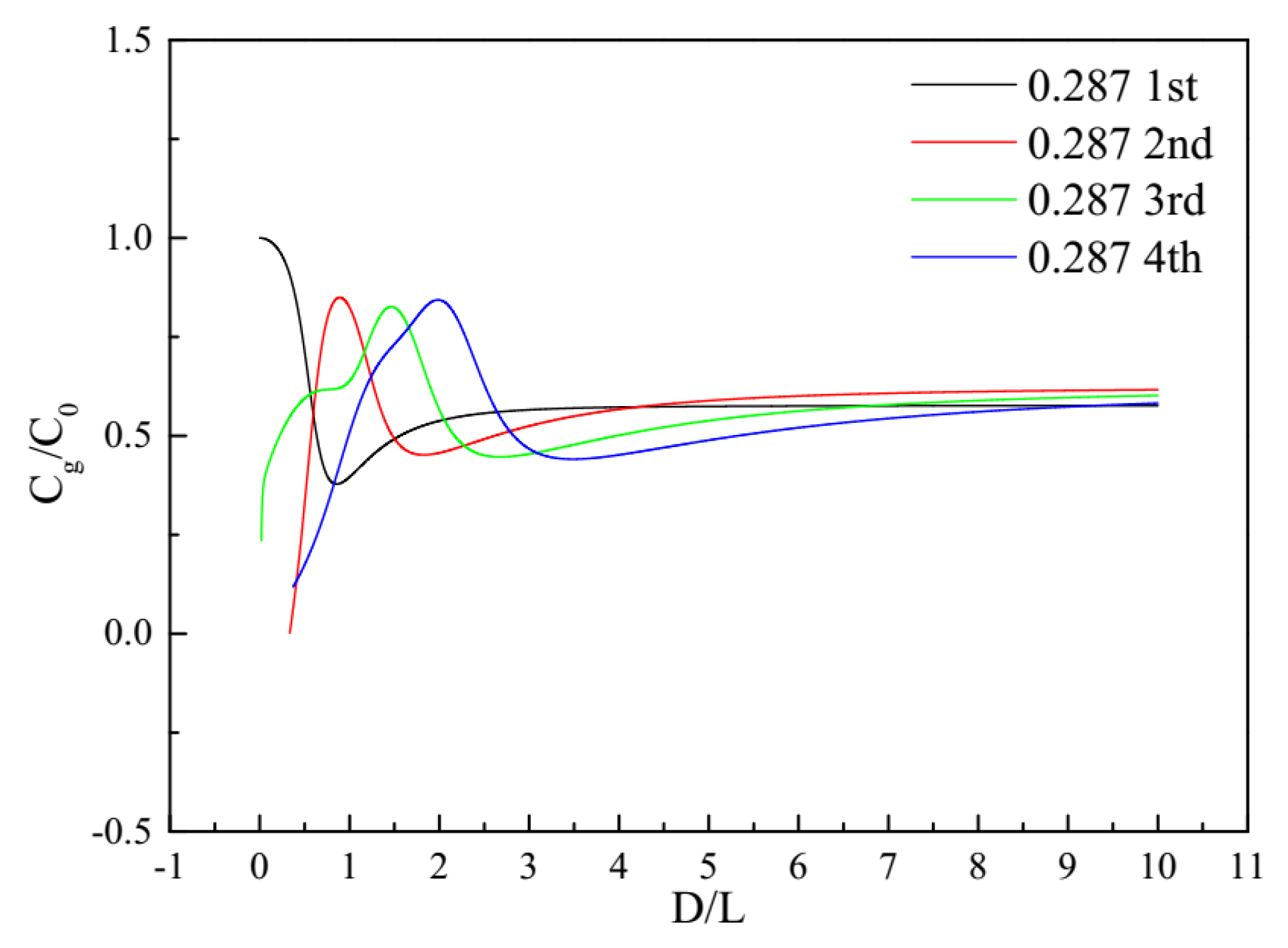
2.1.2. Group Velocity Curve

The phase velocity curve shows the propagation velocity of the equal phase plane of each frequency component of the stress wave. The elastic stress wave excited by an explosion shock wave at the pressure bearing end face of the pressure bar contains rich frequency components. The components with similar frequency will form a wave packet when they propagate. The propagation velocity is called group velocity, which describes the process of energy transmission. The relationship between group velocity and phase velocity is

$$C_g=C+\gamma \frac{dC}{d\gamma }$$

(2)

The group velocity is dimensionless to the elementary theoretical wave velocity, and formula (2) is transformed into

$$\frac{C_g}{C_0}=\frac{C}{C_0}+\frac{D}{L}\frac{d\left(C/C_0\right)}{d\left(D/L\right)}$$

(3)

According to formula (3), the group velocity curve can be calculated from the phase velocity curve shown in Figure 3. It can be seen from Figure 4 that the group velocity curve is non monotonic, and the stress waves of different wavelengths may have the same group velocity. The first-order group velocity curve shows a character of decrease followed by slow increase, which can be summarized as low-frequency fast, medium-frequency slow, and high-frequency approximating constant velocity. In the case of low frequency, $C_g/C_0=1$, that is, the wave packet propagation velocity is consistent with the elementary theoretical wave velocity. When the intermediate frequency part is $D/L=0.857$, the group velocity decreases to the minimum value of $C_g/C_0=0.378$. With further decrease of wavelength, the group velocity gradually converges to $C_g/C_0=0.576$.

The phase velocity of the low frequency component of the second-order and above propagation modes is more than $C_0$, but its group velocity is always less than $C_0$. In the low frequency part of the second-order group velocity curve $D/L<0.334$, $C_g/C_0<0$, the wave packet cannot forward propagation along the bar, that is, there is a low-frequency cutoff phenomenon. $D/L\in \left(0.334,0.891\right]$ part increases monotonically, and the peak group velocity is $C_g/C_0=0.850$. The $D/L\in \left(0.891,1.825\right]$ part monotonically decreases, and the minimum group velocity is $C_g/C_0=0.452$. Part of $D/L\in \left(1.825,10\right]$ increases monotonously slowly to $C_g/C_0=0.616$.

Table 2. Summary of peak, valley, and asymptotic values of the first to fourth order group velocity curves of Poisson’s ratio of 0.287.

Order	Non-Dimensional Number	Peak Value	Valley Value	Asymptotic Value
First	$D/L$	0	0.857	10
	$C_g/C_0$	1	0.378	0.576
Second	$D/L$	0.891	1.825	10
	$C_g/C_0$	0.850	0.452	0.616
Third	$D/L$	1.465	2.677	10
	$C_g/C_0$	0.826	0.447	0.602
Fourth	$D/L$	1.985	3.488	10
	$C_g/C_0$	0.843	0.441	0.583

is a summary of the peak, valley, and asymptotic values of the first to fourth order group velocity curves. The frequency corresponding to the peak value and valley value of each order group velocity increases in turn.

2.1.3. Relationship Between Normalized Frequency and Propagation Time

For a stress wave of a certain frequency, the time period is

$$T=1/f=L/C$$

(4)

Define the time for the elementary theoretical elastic wave to propagate from the center to the edge of the pressure bar as

$$T_a=a/C_0$$

(5)

Divide Equation (5) by Equation (4) to get

$$T_a/T=\frac{fa}{C_0}=\frac{C}{L}\frac{a}{C_0}=\frac{\left(D/L\right)\left(C/C_0\right)}{2}$$

(6)

The energy of the stress wave propagates forward at the group velocity $C_g$ in the pressure bar, so the ratio of the time $t^{\prime }$ when the wave energy propagates to a certain position $z$ in the bar and the time $0.5T_0$ that the elementary theoretical wave propagates to the same position is the normalized propagation time

$$\frac{t^{\prime }}{0.5T_0}=\frac{z/C_g}{z/C_0}=\frac{C_0}{C_g}$$

(7)

Both of the normalized frequency parameters $fa/C_0$ described by Equation (6) and the normalized propagation time parameters $t^{\prime }/0.5T_0$ described by Equation (7) can be obtained by simple calculation of the phase velocity curve (Figure 3) and group velocity curve (Figure 4) and their independent variable $D/L$. Figure 5 is the first to fourth orders of normalized frequency and propagation time curve when Poisson’s ratio is 0.287. Assuming that there are no dispersion effects of various orders in the bar, a vertical line should be shown in Figure 5 and the abscissa should be 1, that is, each frequency component in the bar propagates at the same velocity and reaches any point in the pressure bar at the same time. However, considering the dispersion effect, each order curve is not a simple vertical line, but presents a more complicated pattern.

2.2. Propagation Mode Analysis Based on the Short-Time Fourier Transform

The stress wave will be excited to propagate along the bar when the pressure-bearing end of the bar is subjected to the action of explosion shock wave or bullet impact. In light of the above research results, there are infinite propagation modes of the stress wave in theory, but in engineering, only the first to fourth orders are generally considered. It is impossible to distinguish whether a propagation mode of the stress wave has only one order or is composed of multiple orders on the basis of a single experiment result of a specific pressure bar. However, the first to fourth order normalized frequencies and the propagation time curves in Figure 5 provide an analysis idea that the time to reach the specified point in the bar of the frequency components with different propagation velocities are in sequence and the short pulse will become the long one with the increase of the propagation distance when the stress wave propagates along the axis of the bar for a certain distance. The mechanical parameters (strain, stress, displacement, or velocity) are measured at a certain point in the bar, where the frequency components and their corresponding arrival time in the signal are obtained by time-frequency joint analysis. Then, comparing those results with the curves shown in Figure 5, one can see which modes of the stress wave are excited in this bar.

In reference [7], the photoelectric signal of the PDV is analyzed by the short-time Fourier transform method, and the pressure waveform can be obtained by multiplying the conversion coefficient given by the elementary theory with the velocity waveform of the free surface of the pressure bar obtained by inverse deduction from the frequency shift. In this paper, the short-time Fourier transform method is used to analyze the free surface velocity waveform of the pressure bar, so that the time-frequency joint spectrum of velocity waveform can be obtained.

In the process of continuous time signal processing, the short-time fourier transform (STFT) is defined as:

$${\mathrm{STFT}}_x\left(t,\Omega \right)={\displaystyle \int x\left(\tau \right)g^{*}\left(\tau -t\right)e^{-j\Omega \tau }d\tau }$$

(8)

where $g\left(\tau -t\right)$ is the window function and $g\left(\tau \right)$ is obtained by moving the window function to the right by t. Equation (8) can be understood as Fourier transform of the signal multiplied by the window function. Since the window function is shifted in the time domain, STFT has both time domain and frequency domain positioning functions. The window function is selected as the Hanning window, also known as the raised cosine window. Compared with the Gaussian window, the main beam width of the spectrum is narrower, thus providing better frequency resolution.

2.3. Proposed Local Phase-Amplitude Joint Correction Method

According to reference [12], first of all, the phase correction is made for the different propagation phase velocities of the elastic stress wave in the bar. The phase when a certain frequency component of the stress wave transmitted to a position $z$ in the pressure bar is

$$\varphi \left(f\right)=2\pi f\frac{z}{C}$$

(9)

Equation (9) indicates that the phase is related to the frequency of the stress wave and the propagation velocity of the frequency, that is, related to the propagation order. Different orders of the same frequency have different phases due to different propagation velocities.

The phase difference from elementary theory is

$${\varphi }^{\prime }\left(f\right)=2\pi f\left(\frac{z}{C}-\frac{z}{C_0}\right)$$

(10)

Adding this phase difference to each frequency component and performing inverse Fourier transform can correct the dispersion caused by different phase velocities.

Taking into account predictions from the Pochhammer–Chree theory for both the variation of axial strain over the bar radius and the relationship between axial stress and strain, reference [18] corrected the amplitude of the measured strain signal on the bar surface to obtain the average stress on the pressure end of the pressure bar.

In this paper, the velocity history curve of the center of the free surface of the pressure bar is measured. It is necessary to derive the relationship between the center velocity of the bar and the average stress on the end surface of the bar so as to correct the non-uniformity of the velocity along the radius of the bar.

According to reference [5], the axial displacement of the bar end is

$$u_z=i\gamma A\frac{J_1\left(ha\right)}{ha}{f}_2{e}^{i\left(\gamma z+\omega t\right)}$$

(11)

The axial velocity is the first derivative of the axial displacement with respect to time

$$u_z^{\prime }=-\gamma \omega A\frac{J_1\left(ha\right)}{ha}{f}_2{e}^{i\left(\gamma z+\omega t\right)}$$

(12)

The axial velocity of the bar center is

$$u_z^{\prime }\left(r=0\right)=-\gamma \omega A\frac{J_1\left(ha\right)}{ha}{f}_2\left(r=0\right)e^{i\left(\gamma z+\omega t\right)}$$

(13)

The axial stress in the bar is

$${\sigma }_{zz}=-2\mu {\gamma }^{2}A\frac{J_1\left(ha\right)}{ha}{f}_1{e}^{i\left(\gamma z+\omega t\right)}$$

(14)

where $A$ is amplitude; $f_1$ and $f_2$ are defined as

$$\begin{array}{l}{f}_1=\left(1+x-\beta x\right)\frac{ha{J}_0\left(hr\right)}{J_1\left(ha\right)}+\frac{1-\beta x}{x-1}\frac{ka{J}_0\left(kr\right)}{J_1\left(ka\right)}\\ f_2=\frac{ha{J}_0\left(hr\right)}{J_1\left(ha\right)}+\frac{1-\beta x}{x-1}\frac{ka{J}_0\left(kr\right)}{J_1\left(ka\right)}\end{array}$$

(15)

In order to obtain the average axial stress in the bar, it is necessary to integrate and average Equation (14)

$$\overline{{\sigma }_{zz}}=-2\mu {\gamma }^{2}A\frac{J_1\left(ha\right)}{ha}\overline{f_1}{e}^{i\left(\gamma z+\omega t\right)}$$

(16)

where $\overline{f_1}$ is defined as

$$\begin{array}{ll}\overline{f_1}& =\frac{2}{a^2}{\displaystyle {\int }_0^{a}r{f}_1}dr=2{\displaystyle {\int }_0^a\frac{r}{a}{f}_1}d\left(\frac{r}{a}\right)\\ & =2{\displaystyle {\int }_0^a\left(1+x-\beta x\right)\frac{ha{J}_0\left(hr\right)}{J_1\left(ha\right)}\frac{r}{a}}+\frac{1-\beta x}{x-1}\frac{ka{J}_0\left(kr\right)}{J_1\left(ka\right)}\frac{r}{a}d\left(\frac{r}{a}\right)\\ & =2\left[1+x-\beta x+\frac{1-\beta x}{x-1}\right]\end{array}$$

(17)

The ratio of the axial velocity of the pressure bar center to the average axial stress is

$$\frac{u_z^{\prime }\left(r=0\right)}{\overline{{\sigma }_{zz}}}=\frac{-\gamma \omega A\frac{J_1\left(ha\right)}{ha}{f}_2\left(r=0\right)e^{i\left(\gamma z+\omega t\right)}}{-2\mu {\gamma }^{2}A\frac{J_1\left(ha\right)}{ha}\overline{f_1}{e}^{i\left(\gamma z+\omega t\right)}}=\frac{C\left(1+\sigma \right)}{E}\frac{f_2\left(r=0\right)}{\overline{f_1}}$$

(18)

Take the reciprocal of the Equation (18) to define the amplitude correction coefficient

$$M=\frac{\overline{{\sigma }_{zz}}}{u_z^{\prime }\left(r=0\right)}=\frac{E}{C\left(1+\sigma \right)}\frac{\overline{f_1}}{f_2\left(r=0\right)}$$

(19)

Equation (19) indicates that the relationship between the axial mean stress and the axial velocity at the center of the bar is related to the propagation phase velocity, or to the propagation mode and frequency of the elastic stress wave. The velocity curve of the center point of the free surface of the pressure bar measured by PDV is analyzed by the short-time Fourier transform method, and the propagation mode is obtained. After that, the amplitude correction coefficient can be solved according to the phase velocity corresponding to each order of the propagation mode given in theory. The combined use of phase correction (Equation (10)) and amplitude correction (Equation (19)) can correct waveform dispersion caused by lateral inertial effects.

This paper proposes a local phase-amplitude joint correction method. The algorithm steps are as follows:

Step 1: Perform a short-time Fourier transform on the axial velocity signal of the bar center to obtain its time-frequency spectrum;

Step 2: Analyze the order of the stress wave propagation mode in the bar according to the time-frequency spectrum and the theoretical curve given in Figure 5;

Step 3: Solve the phase correction coefficient matrix and amplitude correction coefficient matrix separately according to the propagation mode;

Step 4: According to the arrival time of the stress wave of a specific frequency transmitted to the end surface of the bar, set the local range (twice the window length) around the frequency-time point in the phase correction coefficient matrix to be effective, and set the rest to 0, that is, the remaining parts do not correct the phase;

Step 5: According to the given upper and lower frequency limits, set the part of the amplitude correction coefficient matrix that exceeds the range to 0, that is, filter out the noise that exceeds the effective frequency range;

Step 6: Repeat steps (3) to (5), calculate the amplitude and phase correction coefficient matrix of all orders of propagation modes in the signal and superimpose and sum them up, then combine the amplitude and phase correction coefficient matrix into a complex amplitude correction matrix;

The complex amplitude correction matrix is multiplied by the time-frequency spectrum of the velocity signal, and then the inverse Fourier transform is performed to obtain the average stress curve of the compression end of the pressure bar.

In this method, at a certain time, only the signal within a small frequency range around the main frequency component that meets the dispersion characteristics is corrected, and the remaining non-dispersed frequency components retain the same phase, thus avoiding the error introduced by the correction of the non-dispersed components.

3. Results and Discussion

3.1. Setup of the Testing System

A testing system was set up for experimental verification after the installation of eight sets of pressure bar sensors, as shown in Figure 6. The testing system consisted of a high-pressure chamber, gas pressure sensors, cylindrical bullet, a laser, a PDV, a serial server, a switch, an oscilloscope, and a computer. The testing process can be described as follows:

Firstly, the piston was pulled to release a cylindrical bullet (Φ 5.93 × 9.92 mm) when the high-pressure gas chamber was pressurized to about 0.4 MPa. As the bullet flew out, the pressure signal, which was recorded by the second channel of the oscilloscope, was measured and used to trigger the oscilloscope.

Secondly, the elastic stress wave was excited and propagated along the bar to the free end when the cylindrical bullet struck the pressure-bearing end of the bar. Then, the Doppler frequency shift laser reflected from the free end of the bar was gathered by the probe and subsequently transmitted to the PDV.

Thirdly, the photoelectric signal generated by the interference of the reference laser and frequency shifted laser was recorded by the first channel of the oscilloscope.

Lastly, the computer adjusted the output power of the laser, controlled the parameters of the oscilloscope, and transmitted the collected signals back to the network for storage and processing through the switch and the serial server.

Figure 7 is a photograph of the testing system. The sampling rate of the oscilloscope was set to 500 MS/s. The laser was a RIO1174-8-31-1 by RIO company (Santa Clara, USA) with a wavelength of 1552.518 nm. The PDV used in this system was self-developed equipment from the previous research of the project group, which is described in detail in Yang’s thesis for a master’s degree [22], and its velocity measurement uncertainty is 0.1 m/s.

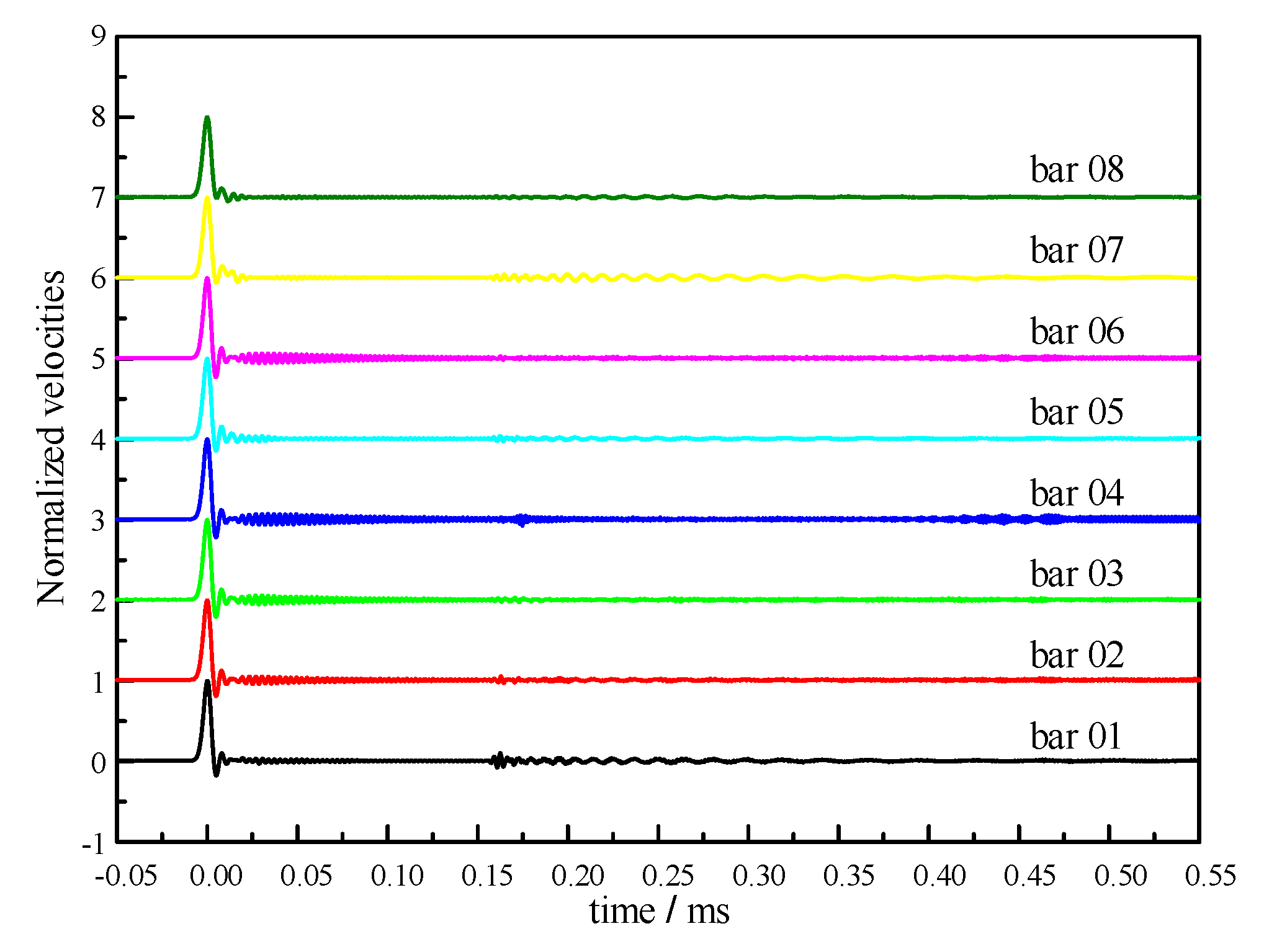
3.2. Preliminary Analysis of Experimental Signals

Figure 8 illustrates the testing signals of the pressure bar 01, the elementary theoretical wave velocity $C_0$ in this bar can be obtained by dividing twice the length of the bar by the period of signal reflection, as the elastic stress wave reflects back and forth between the front and rear end and the length of the bar is known (1500 mm).

Table 3. The preliminary results of the pressure bar obtained by the testing experiment.

Number of Bar	Peak Time (ms)	Reflection Period (μs)	$\mathbf{Wave} \mathbf{Velocity} {\mathit{C}}_0(\mathbf{km}/\mathbf{s})$	Conversion Coefficient (MPa/ms−1)
01	3.666	570.42	5.2595	20.51
02	3.394	571.08	5.2537	20.49
03	3.897	570.67	5.2577	20.51
04	3.612	570.46	5.2589	20.51
05	3.903	570.49	5.2591	20.51
06	3.902	570.29	5.2610	20.52
07	3.637	570.29	5.2610	20.52
08	4.036	570.65	5.2578	20.51
Average	-	570.54	5.2586	20.51
standard deviation	-	0.24	0.0022	0.01

summarizes the experimental results of eight pressure bars, where the average wave velocity is 5.2586 km/s and the standard deviation is 2.2 m/s. Table 3 also gives the free surface velocity–pressure conversion coefficient ($k={\rho }_0{C}_0/2,{\rho }_0=7800\mathrm{kg}/{\mathrm{m}}^3$), calculated from the elastic wave velocity according to the elementary theory.

Figure 9 summarizes the waveforms within the first peak intervals of the eight bars obtained from the testing experiments without containing the subsequent reflected signals. The curves’ baselines are shifted, and the peaks are normalized and then aligned to time zero. It can be seen that the first peaks are followed by high-frequency oscillations, amongst which the large amplitude appears at about 0.16 ms.

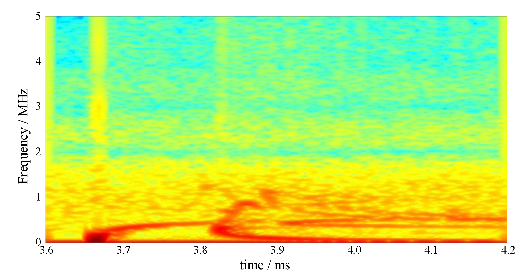
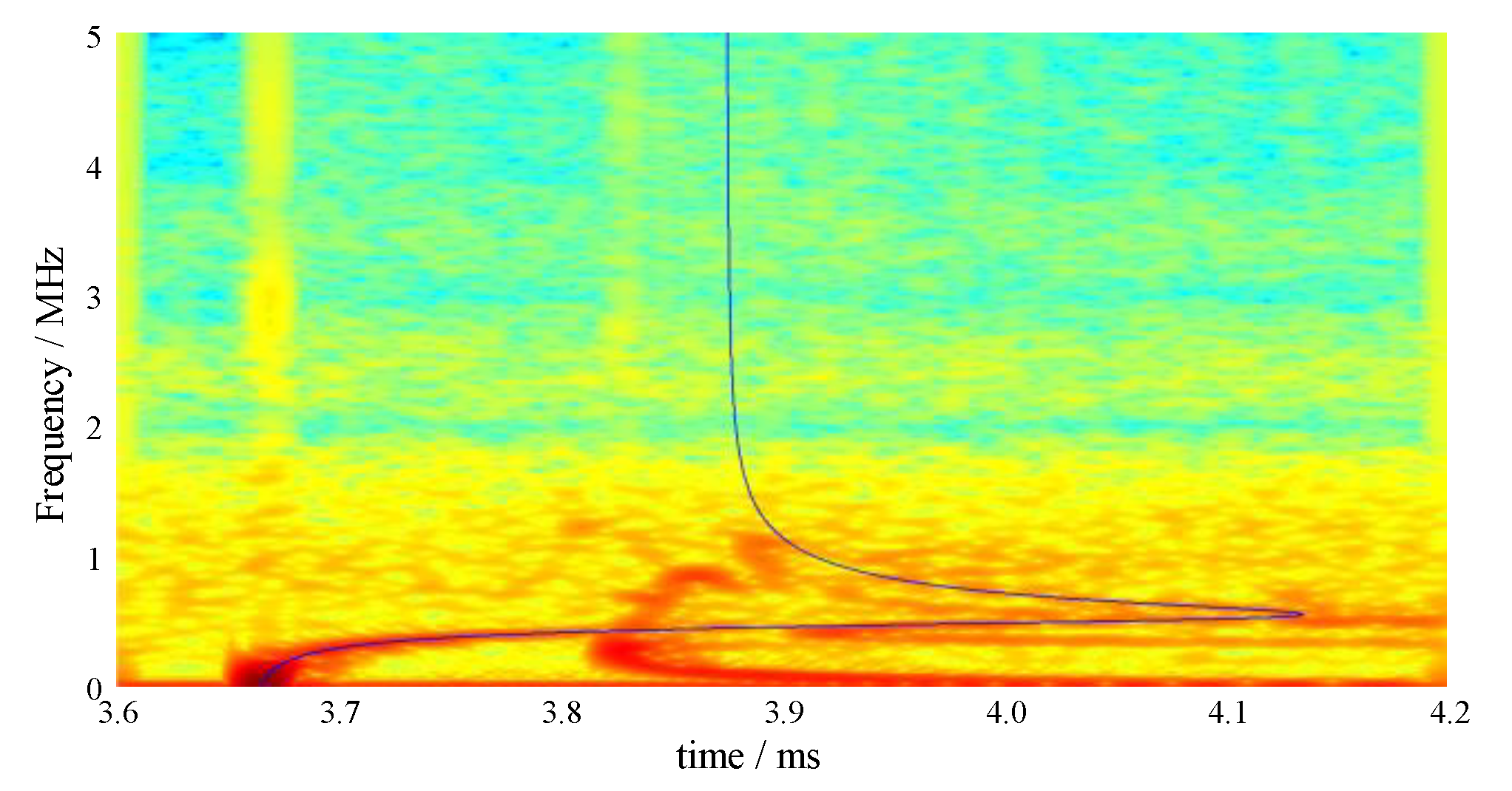
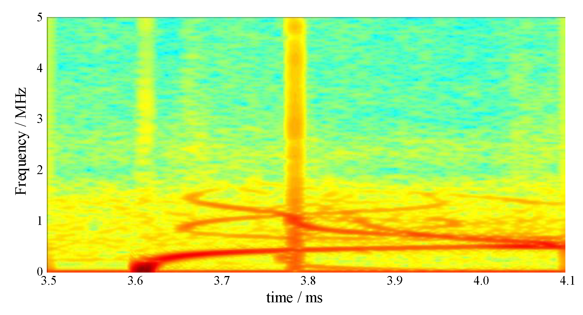
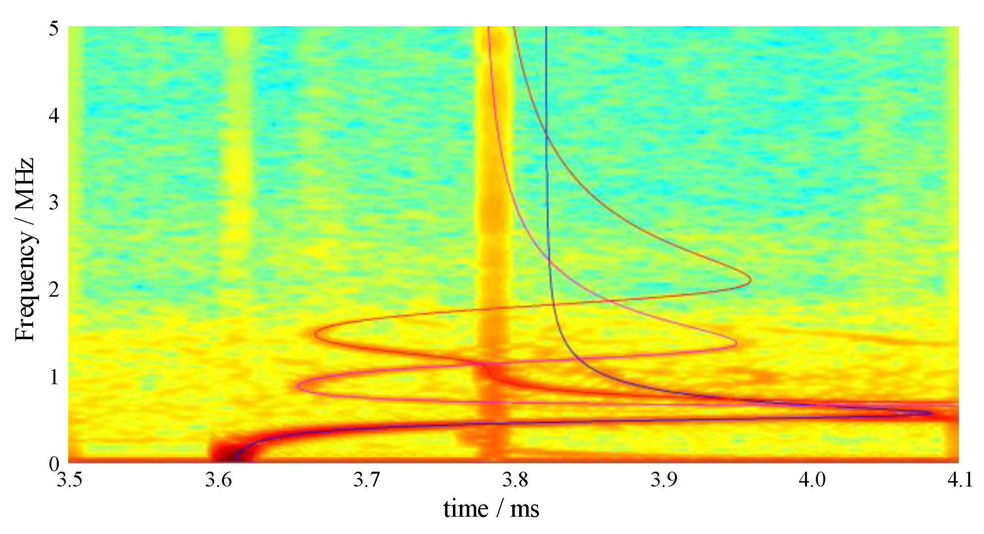
3.3. Propagation Modes Analysis

The self-made data processing program was used to process the velocity signals of each pressure bar in Figure 9 (the signal sampling rate was 10 MS/s). Time-frequency joint spectrums were then obtained by using FFT. The FFT length of STFT was set as 8192 sampling points, the window length was 301 sampling points, and the moving step size was 1 sampling point. Figure 10 shows typical time-frequency joint spectrums of the free surface velocity of bars 01.

The time of elastic wave propagation to the free end of the bar 01 can be obtained by the elementary theory as in Equation (20), where the length of the bar is 1500 mm and the corresponding elastic wave velocity given in Table 3 is 5.2595 km/s.

$$0.5T_0=z/C_0=1500/5.2595=285.2 \mathsf{\mu }\mathrm{s}$$

(20)

The diameter and radius of the pressure bar are 6 mm and 3 mm respectively, substituting those values into Equation (6):

$$\frac{fa}{C_0}=\frac{3 \mathrm{mm}}{5.2595 \mathrm{km}/\mathrm{s}}f=\frac{f}{1.753 \mathrm{MHz}}$$

(21)

The abscissa and ordinate in Figure 5 are converted into time and frequency by Equations (20) and (21), then the time-frequency joint spectrum is obtained after a 3.666 ms-shift on the time axis as shown in Figure 11. It can be seen that the time-frequency components in the measured signal are in agreement with the first-order propagation mode given by theory, but with a lower frequency upper limit (less than 1 MHz). In addition, the frequency components between 3.8 ms and 3.9 ms are different from the longitudinal stress wave given by the theory, which is determined as a bending wave and will not be discussed in this paper. The results demonstrated that the axial velocity of the center of the pressure bar 01 is dispersed according to the first-order propagation mode.

As for the other sets of pressure bar sensors except bar 04, the elastic stress waves are similar to that of bar 01 and follow the first-order propagation modes, while the spectrum of bar 04 represents a more complex pattern as illustrated in Figure 12.

A similar analysis method as that used on bar 01 was applied on data from bar 04. Values of size and elastic wave velocity of bar 04 were used in the corresponding formulas, meanwhile, the theoretical propagation mode curves of corresponding orders were drawn in the time-frequency diagram. As shown in Figure 13, the first three propagation modes are excited and in good agreement with the theoretical ones.

Table 4. The frequency range of the first to third order modes of bar 04.

Order	Lower Frequency Limit /MHz	Upper Frequency Limit /MHz
First	0	1.0
Second	0.6	1.5
Third	0.6	1.8

shows the frequency range of the first three propagation modes.

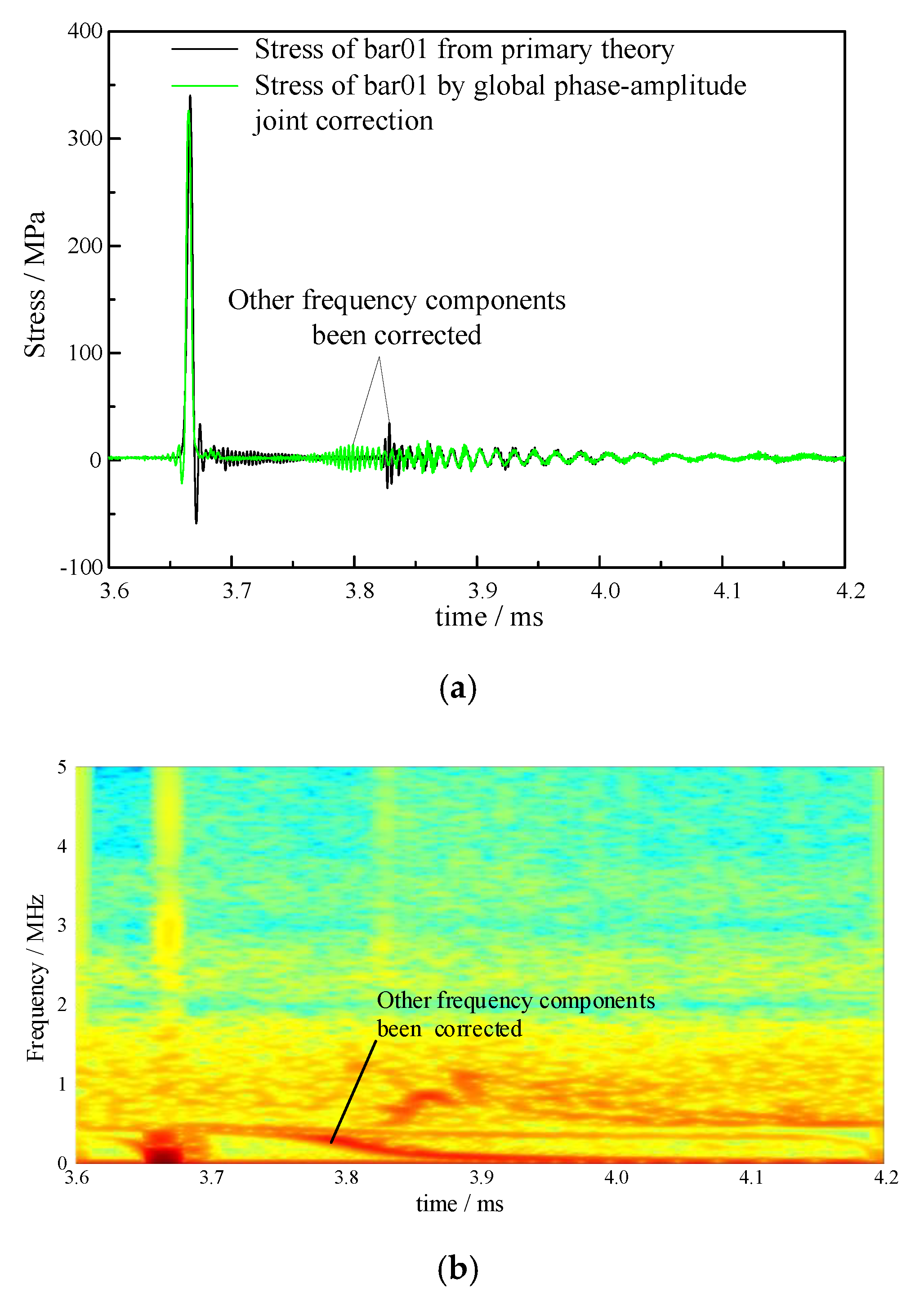
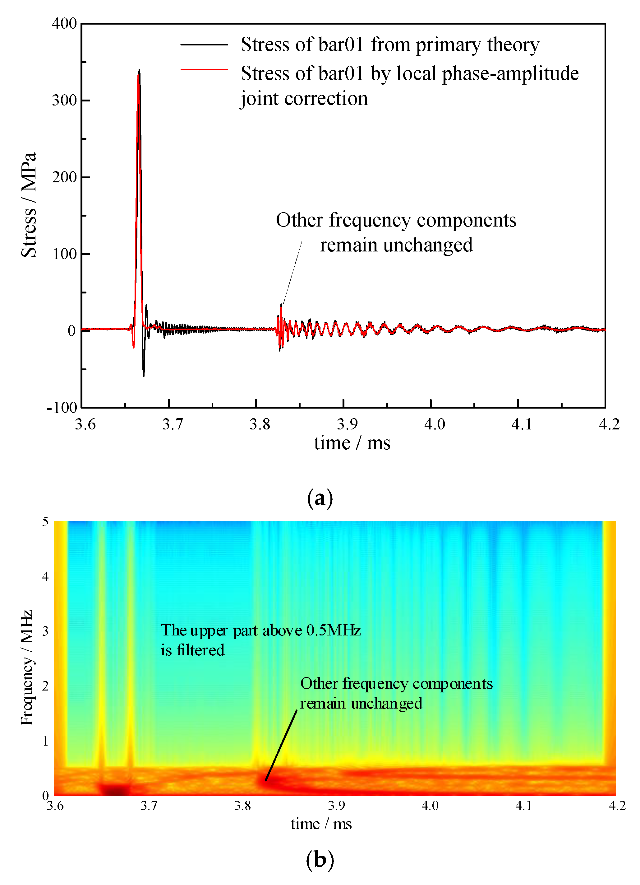
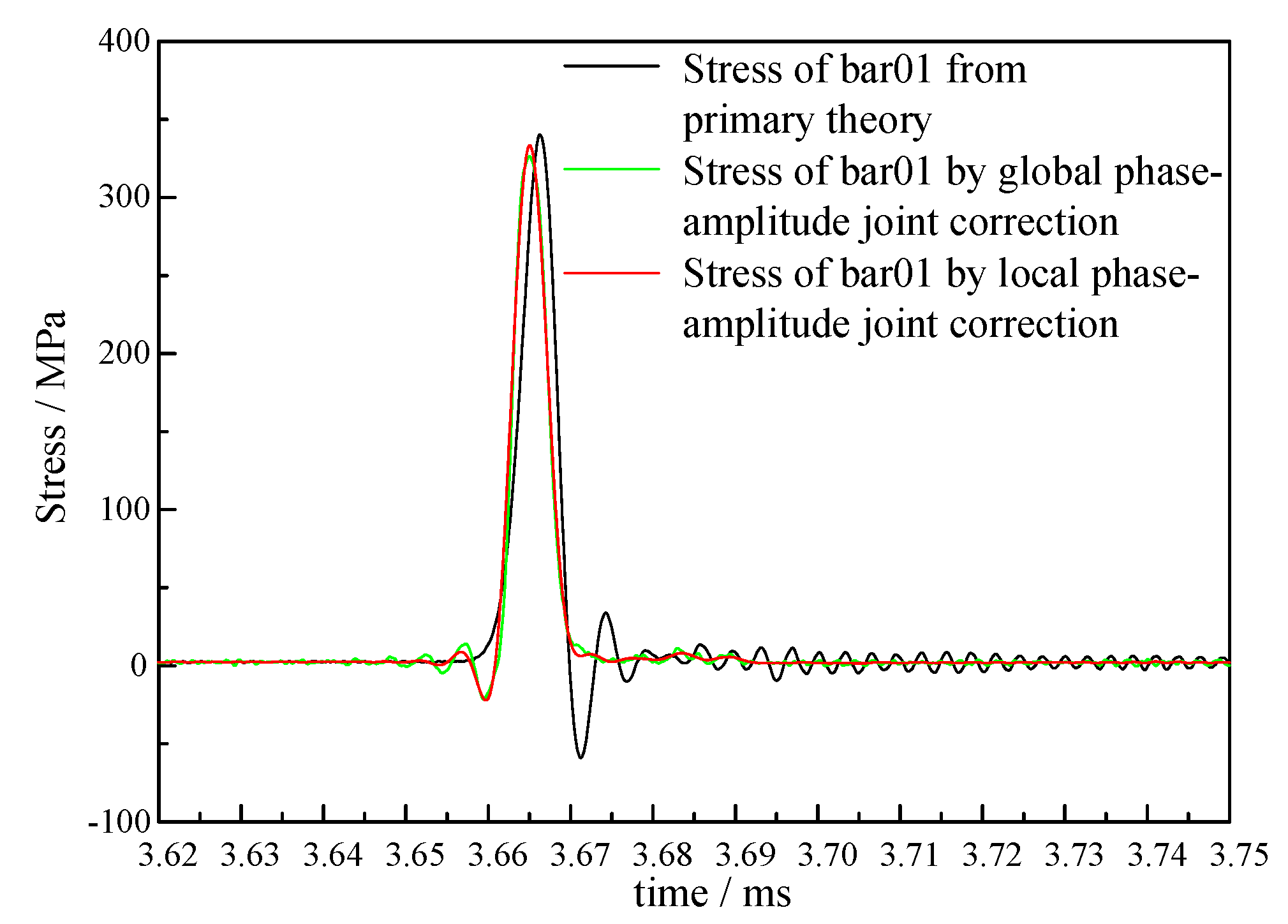
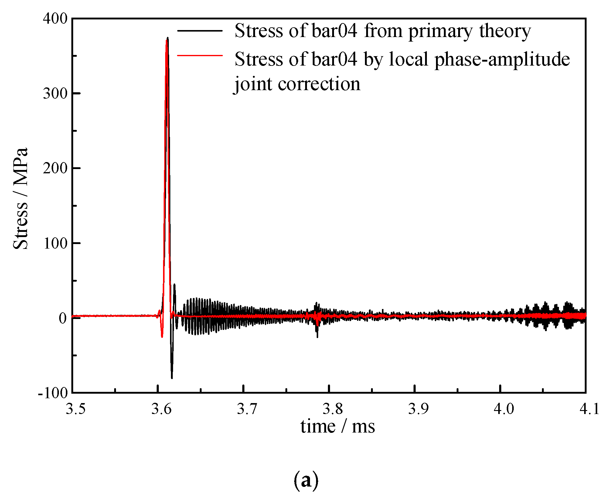
3.4. Local Phase-Amplitude Joint Correction

For comparative analysis, the velocity signal of the pressure bar 01 was first corrected for dispersion using the global phase-amplitude joint correction method in the first-order propagation mode. The global phase-amplitude joint correction method corrected the phase and amplitude of frequency components over the full duration of signal. The corrected result is shown in Figure 14. For comparison, the time was selected to be aligned with the original signal, and the upper limit of the phase correction frequency was set to be 0.5 MHz. In Figure 14a, the black line is the stress curve obtained by multiplying the velocity by the conversion coefficient given by the elementary theory (Table 3), and the green line is the stress curve obtained by the global phase-amplitude joint correction. It is noteworthy that the oscillation around 3.83 ms is moved forward, and this part of the oscillation is not the frequency characteristic described by the first-order propagation mode of the axial stress wave, indicating that the global phase-amplitude joint correction method will introduce new errors.

The local phase-amplitude joint correction method proposed in this paper was then used to correct the velocity signal to obtain the average stress signal of the compression surface of the pressure bar. The upper frequency limit was set to 0.5 MHz, signals beyond this frequency limit were considered to be noise and were filtered out. Signals in the frequency band were not phase-corrected, except for the first-order propagation mode. As can be seen from Figure 15, the diffuse signal between 3.67 ms and 3.82 ms is well corrected, while impacts on oscillations around 3.83ms are minimal, therefore, the additional errors that were introduced can be neglected.

Figure 16 compares the stress curve of the end face under pressure obtained by elementary theory, global phase-amplitude joint correction, and local phase-amplitude joint correction. It can be seen that the local phase-amplitude joint correction method led to lower baseline oscillations in the signal and showed a better correction result than those of the global method. The rising edge of the stress signal given by the elementary theory is 4.13 μs, and the rising edge after local correction is 2.70 μs (10~90%). Moreover, a negative oscillation occurs at 3.66 ms at the leading edge of the main peak, indicating that the algorithm should be further improved.

The local phase-amplitude joint correction method was further used to process the signal of the bar 04. The frequency range of each order propagation mode was set by parameters in Table 4. Figure 17a compares the corrected curve and the curve given by the elementary theory. It can be seen that the amplitude of the oscillation following the main peak is greatly reduced, while the frequency component of the non-axial stress wave around 3.785 ms is minimally influenced. Figure 17b shows the time-frequency joint time spectrum of the corrected stress signal. Components higher than 1.8 MHz were filtered out, while the first-order propagation mode still has components with lower amplitude. Further improvement of the algorithm is needed. The second and third-order propagation modes are well corrected, and the local positions marked in the figure appear as light blue with lower energy. Figure 17c is the local magnification of the bar-end average stress curve and the stress curve given by the elementary theory near the main peak. The rising edge of the stress signal given by the elementary theory is 4.09 μs, and the rising edge after local correction is 2.70 μs (10%~90%). Similar to results of the pressure bar 01, the negative peak oscillations of the main peak in the pressure bar 04 are present.

4. Conclusions

In this paper, the elastic stress wave propagation characteristics in a cylindrical pressure bar were investigated based on the Pochhammer–Chree theory. A method of analyzing the free surface velocity of the pressure bar using short-time Fourier transform was proposed to analyze the propagation mode. In addition, a local phase-amplitude joint correction method was proposed to convert the measured velocity into the average reflected pressure of a shock wave, excluding the components of the non-axial elastic wave.

The conclusions are as follow:

(1)

The propagation mode analysis method based on short-time Fourier transform is intuitive and clear and gives all the propagation modes of the axial elastic stress wave.

(2)

In the eight sets of pressure bars, the pressure bar 04 excited the first three orders of the propagation mode, while the stress waves in the remaining pressure bars propagated in the first-order mode.

(3)

The local phase-amplitude joint correction method only corrected the frequency component corresponding to the propagation mode excited in the pressure bars.

(4)

Testing experiments verify the feasibility of the correction method. The rising edges of the pressure bars 01 and 04 are corrected from 4.13 μs and 4.09 μs to 2.70 μs, respectively.

In summary, the elastic stress wave propagation mode analysis and the local phase-amplitude joint correction method proposed in this paper can provide more accurate results in reflected near-field blast pressure measurements for the study of new explosives.

References

1. Hopkinson, B. A method of measuring the pressure produced in the detonation of high explosives or by the impact of bullets. Philos. Trans. R. Soc. Lond. Ser. A Contain. Pap. Math. Phys. Character 1914, 213, 437–456. [Google Scholar]
2. Cloete, T.J.; Nurick, G.N. Blast characterization using a ballistic pendulum with a centrally mounted hopkinson bar. Int. J. Prot. Struct. 2016, 7, 367–388. [Google Scholar] [CrossRef]
3. Rigby, S.E.; Knighton, R.; Clarke, S.D.; Tyas, A. Reflected near-field blast pressure measurements using high speed video. Exp. Mech. 2020, 1–14. [Google Scholar] [CrossRef]
4. Clarke, S.D.; Fay, S.D.; Warren, J.A.; Tyas, A.; Rigby, S.E.; Elgy, I. A large scale experimental approach to the measurement of spatially and temporally localised loading from the detonation of shallow-buried explosives. Meas. Sci. Technol. 2014, 26, 15001. [Google Scholar] [CrossRef]
5. Davies, R.M. A critical study of the hopkinson pressure bar. Philos. Trans. R. Soc. Lond. Ser. A Math. Phys. Sci. 1948, 240, 375–457. [Google Scholar]
6. Hauser, F.E. Techniques for measuring stress-strain relations at high strain rates. Exp. Mech. 1966, 6, 395–402. [Google Scholar] [CrossRef]
7. Yang, J.; Li, Y.; Zhang, D. Measuring technique of reflected blast wave pressure based on pressure bar and photonic doppler velocimeter. Acta Armamentarii 2017, 38, 1368–1374. [Google Scholar]
8. Pochhammer, L. On the propagation velocities of small oscillations in an unlimited isotropic circular cylinder. J. Reine Angew. Math. 1876, 81, 324–326. [Google Scholar]
9. Chree, C. The equations of an isotropic elastic solid in polar and cylindrical coordinates, their solution and application. Trans. Camb. Philos. Soc. 1889, 14, 250–369. [Google Scholar]
10. Bancroft, D.; Jacobs, R.B. An electrostatic method of measuring elastic constants. Rev. Sci. Instrum. 1938, 9, 279–281. [Google Scholar] [CrossRef]
11. Yew, E.H.; Chen, C.S. Experimental study of dispersive waves in beam and rod using fft. J. Appl. Mech. 1978, 45, 940–942. [Google Scholar] [CrossRef]
12. Gorham, D.A. A numerical method for the correction of dispersion in pressure bar signals. J. Phys. E Sci. Instrum. 1983, 16, 477–479. [Google Scholar] [CrossRef]
13. Follansbee, P.S.; Frantz, C. Wave propagation in the split hopkinson pressure bar. J. Eng. Mater. Technol. 1983, 105, 61–66. [Google Scholar] [CrossRef]
14. Gong, J.C.; Malvern, L.E.; Jenkins, D.A. Dispersion investigation in the split hopkinson pressure bar. J. Eng. Mater. Technol. 1990, 112, 309–314. [Google Scholar] [CrossRef]
15. Lifshitz, J.M.; Leber, H. Data processing in the split hopkinson pressure bar tests. Int. J. Impact Eng. 1994, 15, 723–733. [Google Scholar] [CrossRef]
16. Zhao, H.; Gary, G.; Klepaczko, J.R. On the use of a viscoelastic split hopkinson pressure bar. Int. J. Impact Eng. 1997, 19, 319–330. [Google Scholar] [CrossRef]
17. Lee, C.K.B.; Crawford, R.C.; Mann, K.A.; Coleman, P.; Petersen, C. Evidence of higher pochhammer chree modes in an unsplit hopkinson bar. Meas. Sci. Technol. 1995, 6, 853–859. [Google Scholar] [CrossRef]
18. Tyas, A.; Watson, A.J. A study of the effect of spatial variation of load in the pressure bar. Meas. Sci. Technol. 2000, 11, 1539–1551. [Google Scholar] [CrossRef]
19. Tyas, A.; Pope, D.J. Full correction of first-mode pochammer-chree dispersion effects in experimental pressure bar signals. Meas. Sci. Technol. 2005, 16, 642–652. [Google Scholar] [CrossRef]
20. Tyas, A.; Watson, A.J. An investigation of frequency domain dispersion correction of pressure bar signals. Int. J. Impact Eng. 2001, 25, 87–101. [Google Scholar] [CrossRef]
21. Rigby, S.E.; Barr, A.D.; Clayton, M. A review of pochhammer-chree dispersion in the hopkinson bar. Proc. Inst. Civ. Eng. Eng. Comput. Mech. 2018, 171, 3–13. [Google Scholar] [CrossRef] [Green Version]
22. Yang, J. The Development of Fiber Displacement Interferometer and Its Applications. Master’s Thesis, University of Science and Technology of China, Hefei, China, 17 May 2012. [Google Scholar]
Figure 1. The sign and discontinuous point distribution of the real part of the function value ( σ = 0.3 ).
Applsci 10 05390 g001
Figure 2. The first-order phase velocity curves of different Poisson’s ratio.
Applsci 10 05390 g002
Figure 3. The first to fourth order phase velocity curves of Poisson’s ratio of 0.287.
Applsci 10 05390 g003
Figure 4. The first to fourth order group velocity curves of Poisson’s ratio of 0.287.
Applsci 10 05390 g004
Figure 5. The first to fourth normal frequency and propagation time curves of Poisson’s ratio of 0.287.
Applsci 10 05390 g005
Figure 6. The diagram of testing system.
Applsci 10 05390 g006
Figure 7. A photograph of the testing system.
Applsci 10 05390 g007
Figure 8. Typical velocity curve of free surface of pressure bar obtained by photonic doppler velocimetry (PDV).
Applsci 10 05390 g008
Figure 9. The testing signal of eight pressure bar sensors.
Applsci 10 05390 g009
Figure 10. Time-frequency joint spectrum of the free surface velocity of bar 01.
Applsci 10 05390 g010
Figure 11. The first order mode included in the time-frequency joint spectrum of bar 01.
Applsci 10 05390 g011
Figure 12. Time-frequency joint spectrum of the free surface velocity of bar 04.
Applsci 10 05390 g012
Figure 13. The first to third order modes included in the time-frequency joint spectrum of bar 04.
Applsci 10 05390 g013
Figure 14. The result of the first order mode global phase-amplitude joint correction of bar 01′s free surface velocity (a) Comparison of corrected stress curve with elementary theory stress curve; (b) Time-frequency joint spectrum of corrected stress curve.
Applsci 10 05390 g014
Figure 15. The result of the first order mode local phase-amplitude joint correction of bar 01′s free surface velocity (a) Comparison of corrected stress curve with elementary theory stress curve; (b) Time-frequency joint spectrum of corrected stress curve.
Applsci 10 05390 g015
Figure 16. Comparison of the stress curve of pressure bar 01 with different methods.
Applsci 10 05390 g016
Figure 17. The velocity signal of pressure bar 04 after joint correction of local phase-amplitude from first to third order propagation mode. (a) Comparison of corrected stress curve with elementary theory stress curve; (b) Time-frequency joint spectrum of corrected stress curve; (c) Comparison of stress curves of pressure bar 04 with different methods.
Applsci 10 05390 g017aApplsci 10 05390 g017b