A Three-Tier Architecture of Large-Scale Wireless Sensor Networks for Big Data Collection

Abstract

In recent years, technological advances and the ever-increasing power of embedded systems have seen the emergence of so-called smart cities. In these cities, application needs are increasingly calling for Large-Scale Wireless Sensor Networks (LS-WSN). However, the design and implementation of such networks pose several important and interesting challenges. These low-cost, low-power devices are characterized by limited computing, memory storage, communication, and battery power capabilities. Moreover, sensors are often required to cooperate in order to route the collected data to a single central node (or sink). The many-to-one communication model that governs dense and widely deployed Wireless Sensor Networks (WSNs) most often leads to problems of network overload and congestion. Indeed, it is easy to show that the closer a node is geographical to the sink, the more data sources it has to relay. This leads to several problems including overloading of nodes close to the sink, high loss rate in the area close to the sink, and poor distribution of power consumption that directly affects the lives of these networks. In this context, we propose a contribution to the problem of LS-WSN energy consumption. We designed a hierarchical 3-tier architecture of LS-WSNs coupled with a modeling of the activities of the different sensors in the network. This architecture that is based on clustering also includes a redeployment function to maintain the topology in case of coverage gaps. The results of the performed simulations show that our architecture maximizes the lifetime than compared solutions.

1. Introduction

Wireless sensor networks (WSNs) have continued to generate a great deal of interest over the past two decades due to the wide range of applications they allow [1,2]. Their autonomy, simplicity of implementation, and miniature appearance make it possible to integrate them into a wide range of small and large-scale applications. Smart cities where information and communication technologies are increasingly used in everyday life offer many opportunities for Large Scale Wireless Sensor Networks (LS-WSNs) applications [3]. Indeed, in the face of strong demographic growth, the main challenge for these cities is to offer high-performance and innovative services that should improve the living environment. More often than not, these cities use technological means such as Internet of Things (IoT), Big Data, Open Data, and Web/mobile applications.

The development and the deployment of electronic sensors and smart IoT devices on street furniture make it possible to interconnect infrastructures, to provide useful information to public and private services and citizens, or to adapt energy expenditure, among other things [4,5,6]. Moreover, data is at the center of the digital development of services. The new models of data collection are becoming more and more efficient (IoT in particular) and the amount of collected data is exponential. This has led to problems concerning the sharing, storage, analysis, and presentation of data. Therefore, Big Data is the term used for massive volumes of data. Also, older models of data storage and processing are no longer suitable. This has led to this phenomenon and new models have been emerging for some years now [7]. Furthermore, the concept of Open Data refers to data that is open to the entire population. Anyone can access, use, distribute, redistribute, mix, or share it without restriction or commercial contribution, but also contribute by adding or creating new data. The essence of Open Data is interoperability, i.e., the ability to freely mix different data sets. This allows the creation of large and complex systems [8]. Finally, internet access and smartphones or tablets allow access to a large number of digital services. These services can be used to inform citizens, conduct research, give opinions, or sometimes take action (e.g., feedback on information, etc.). The energy consumption of his or her household can enable a citizen to take action to reduce its bill and consequently to carry out a “green” act. Web and mobile applications also allow public services to interact with citizens, soliciting their opinions and actions. In addition, these applications also allow to restitute and sometimes act on the information collected and analyzed on the sensors located on the street furniture.

Furthermore, in the day-to-day management of smart cities, general data play an important role. However, big data remains a problem in its own right. Therefore, this mass of data constitutes one of the major challenges of moderate computing [9,10,11,12,13]. It is almost impossible to collect and then process this data using conventional computer systems. However, for smart cities, most of the literature [14,15] agrees that once collected and processed, these data can support or improve most of the services offered in smart cities (operation of renewable electricity production facilities, real-time status of public distribution networks, monitoring of road traffic, measurement of pollution levels, etc.).

Although LS-WSNs are a preferred solution for data collection and processing, these networks are little or not used to our knowledge for collecting big data across smart cities. This remains an interesting challenge that we wish to take up through our work. However, the design and implementation of LS-WSNs pose several important and interesting challenges [1,16,17,18,19]. These low-cost, low-power devices are characterized by limited computing, memory storage, communication, and battery power capabilities.

The main challenges in achieving such networks are scaling network protocols for a large number of nodes, designing simple and efficient protocols for different network operations, and designing energy-saving protocols. The objective of this paper is to involve the sensors of a multi-level architecture of heterogeneous LS-WSNs in the process of maximizing network lifetime. This is done by proposing a model that should structure the functioning of the different sensors. A LS-WSN consists of several hundred thousand sensors with low battery and computing capacity and a very small number of base stations (mostly stationary) with unlimited battery and high computing capacity. The best way to take advantage of these devices is to allow them to operate autonomously as long as possible. In this paper, we present a unified multi-level LS-WSN architecture that encompasses the physical and logical modeling of the sensors, the data collection process, and the data routing strategy.

Generally, improving lifetime is an important issue when deploying WSNs on a large scale. Indeed, these networks are composed of autonomous sensors that are mostly powered by batteries that are often difficult to recharge or replace. The challenge that animates us in this document is to ensure the operation of the LS-WSN for several years without any intervention related to the energy resources of the sensors. In order to maximize the lifetime, we rely on the structuring of the network according to a multi-level architecture. We proposed a two-stage solution. The first consists of a proposed deployment of the LS-WSN following a three-tier architecture as described in [16] and the second, based on a heuristic, which proposes a model of the communication of the different sensors of the network that guarantees the scaling and considerably reduces the consumption of the whole network. In simulations, we have used the network to collect big data in smart cities. The main objective of this research is to highlight the contribution of the LS-WSN communication system modeling in the optimization of the energy consumption of the sensors, which also amounts to the optimization of the network lifetime. In summary, our main contributions are:

• Comparative study of LS-WSNs deployment architectures;
• Designing a three-tier architecture dedicated to LS-WSNs;
• Modeling of sensor communication according to the three-thirds LS-WSN architecture;
• Validation by simulation of our architecture on a scenario of big data collection in a smart city;
• Validation of the performance of the architecture by a comparative test with existing models;
• Analysis and interpretation of results

The rest of the paper is organized as follows: Section 2 presents the related work that includes the problem of LS-WSNs for big data collection; Section 3 presents our three-tier architecture for a LS-WSN deployment; Section 4 presents the proposed model and its implementation at different levels of the network; Section 5 presents the results and discussions; and the conclusion and future research is presented in Section 6.

2. Related Work

2.1. Problem of Ls-Wsn for Big Data Collection

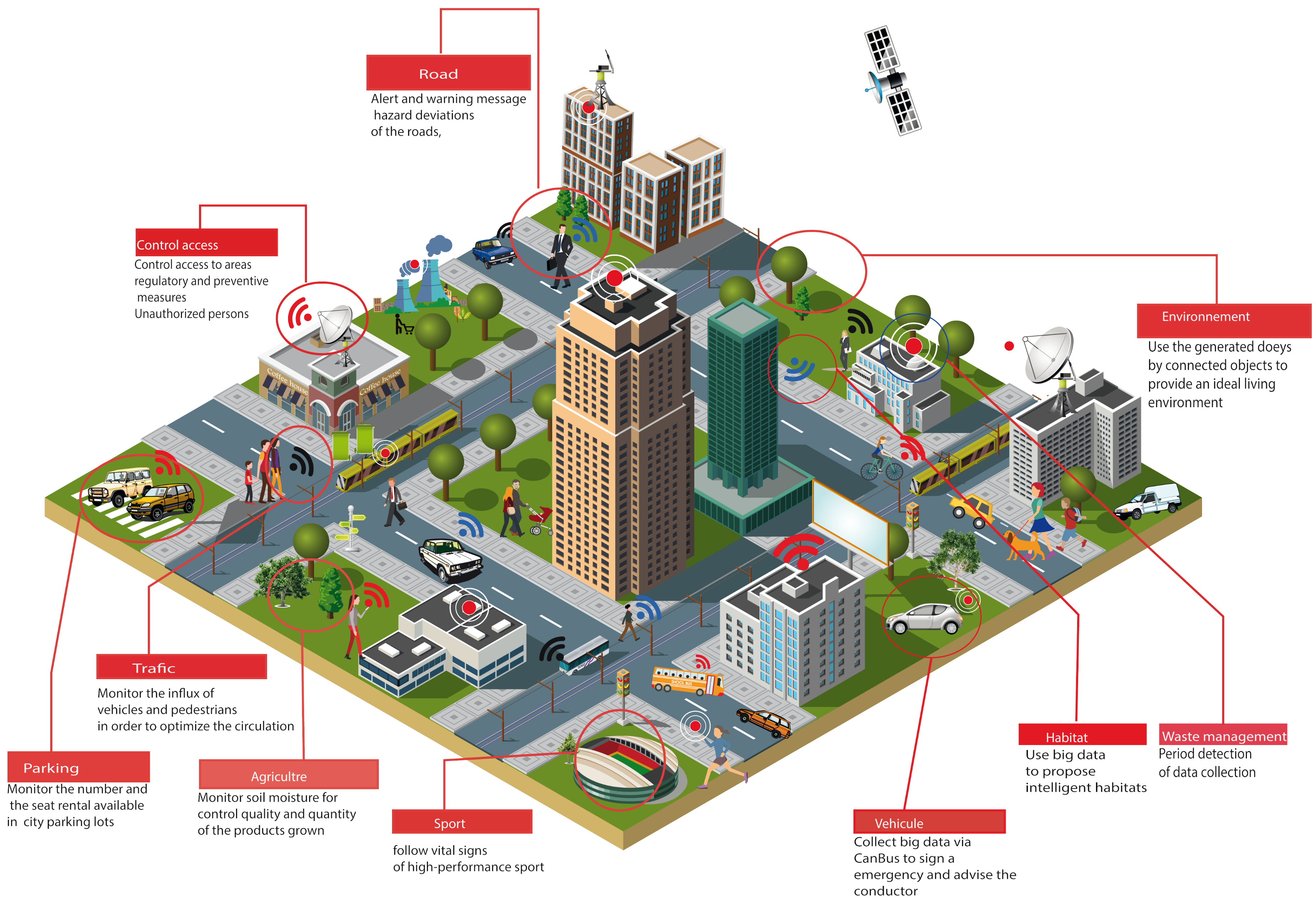
LS-WSNs are a set of thousands of low-cost, low-power sensors with limited computing, memory storage, communication and battery power capabilities that often have to cooperate in order to route the collected data to a single central node or sink [1,20]. In recent years, these networks have seen their fields of application broaden to penetrate smart cities (see Figure 1), in several areas including monitoring, measurement and data collection, health applications, and precision agriculture. For these types of applications, the general purpose of a LS-WSN is the collection of a set of data, from an extended environment, in order to route them, through multi-hop routing, to processing points called base stations (or sinks).

However, the technological challenges to be met by these networks are numerous; beyond the continuous miniaturization of these objects, their communication capacities have given rise to many problems. Unlike traditional networks that seek to guarantee a good quality of service, LS-WSNs place great importance on energy consumption, which remains the major concern of the protocols proposed for these networks [16,18]. Indeed, sensors are often equipped with non-rechargeable batteries that are difficult to replace. The survival and performance of such a network, therefore, depend on the lifetime of the batteries in its nodes. The main task of a sensor, deployed in an area of interest, is to detect events or measure a quantity, or calculate and aggregate the collected data and transmit it to the Base Station (BS). Energy consumption therefore mainly concerns three operations: acquisition, communication, and data processing. The energy consumption by the acquisition operation depends on the nature of the application. For instance, a sporadic or periodic detection could consume less energy than permanent monitoring of an event. Data communication generally consumes more energy than other operations and therefore needs to be well-controlled [21,22].

In smart cities, where almost all the services offered are provided by means of a computer system to such an extent that these cities are considered to be one of the main sources of big data in the world. There is a lot of interest in this data in many sectors. However, in view of the intrinsic characteristics of big data, still considered one of the great challenges of modern computing, collecting them using LS-WSNs is a twofold challenge that we are seeking to meet. Although such a solution is, to our knowledge, a first. The challenges are many. For us, it is a question of proposing a logical architecture for LS-WSN deployment capable of responding to the scale-up and maximizing the life of the network. To do so, in the context of this document, we have chosen to collect big data generated by persons from their multiple activities, and the data from their environment. As set out in our research problematic, we need to review the literature on the different approaches to deploying WSNs in order to adapt it to our context, and then propose mechanisms that will allow us to maximize the life span of the network.

2.2. Architectures for Large-Scale Wireless Sensor Networks Deployments

The application stakes of LS-WSNs are huge [12,14,15]. However, the real challenge for these networks is to manage to operate for several years without any major external intervention. In these types of networks, it is impossible to organize the deployed sensors according to a centralized architecture (too costly in energy) or to preserve a flat communication structure because several issues are even more critical with the transition to scale [1,23]. Among other things, the size of the routing table per sensor must be reduced, - the number of (re-)transmissions, - the bandwidth occupation, - the power consumption per node. Therefore, the introduction of a hierarchy in LS-WSNs is an option that is increasingly being considered in order to maximize the lifetime of the sensors and thus the lifetime of the network. This results in the creation of a virtual logical topology over the physical topology of the network.

The logical topologies of LS-WSN proposed in the literature are numerous and take into account the physical architecture of the network. In this study, we focus on the topologies based on clustering [24,25]. Depending on the sensor deployment mode (deterministic or random), the cluster-head election process, the cluster size, and the network operating model, several clustering approaches have been proposed in recent years.

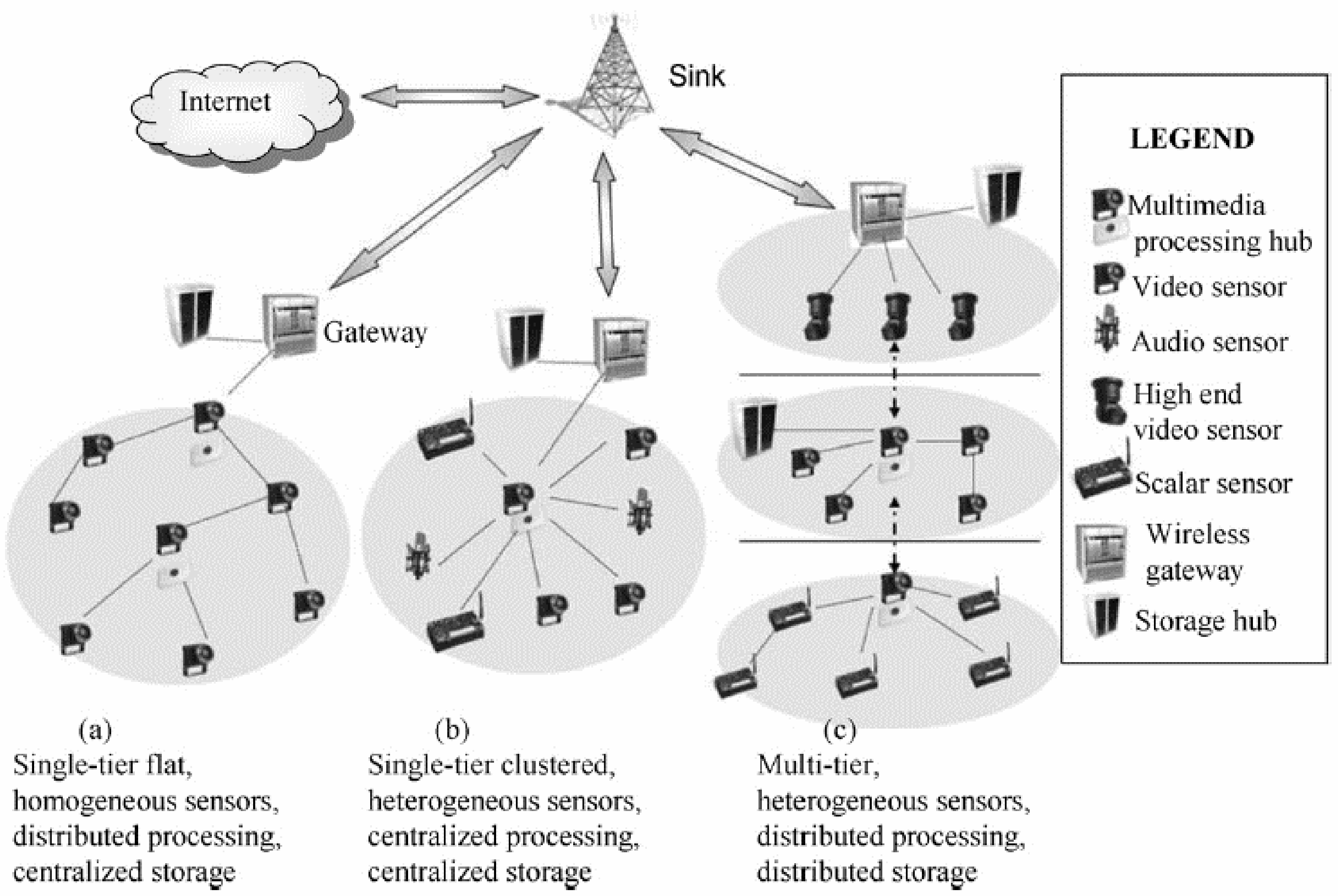
In [26], a reference study on WSN architectures where the authors propose a taxonomy of logical topologies of WSN illustrated by Figure 2. It is composed of an architecture with: a “Single-tier flat” capture level, a “Single-tier clustered” capture level and finally several “multi-tier flat” capture levels in a cluster. The choice of an architecture is most often dictated by the nature of the application to be deployed but also by the nature of the sensors to be used. Moreover, the single capture level architecture is the most widely used in many works [27,28,29]. It is usually a network of homogeneous sensors with distributed job processing and centralized storage. Each sensor in the network performs all the tasks required by the application (e.g., capturing temperature, acceleration, motion, etc.). A variant of this architecture is the single-sensor architecture but the data collecting sensors are grouped in a cluster. There are heterogeneous sensors with processing and storage that are centralized at a dedicated central node, as shown in Figure 2.

The architecture with multiple sensor levels consists of heterogeneous sensors with the processing and storage of data distributed across different levels. In such an architecture, tasks are distributed between the different sensors. It is therefore not useful for a sensor to embark on all the desired functionalities of the network (the nodes are classified according to their capacities: processing, capture, storage, nodes constrained and less constrained in energy, etc.). For example, for such a network, sensors with limited energy resources will be able to perform simple tasks such as temperature capture, motion detection, low-resolution image capture, etc.). On the other hand, sensors with large energy and computational resources will handle more complex tasks, such as high-resolution cameras that can be woken up at the supervisor’s request for recognition and localization. In order to achieve the common monitoring objective, the different sensors must cooperate (according to a suitable communication protocol) to reach the well.

The major disadvantage of the architectures described above is that they shorten the lifetime of the network. Numerous researches [17,28,29,30] have shown that these architectures pose a problem of the rapid depletion of the energy resources of the sensors located in the vicinity of the well. The energy consumption of the network is not uniform throughout the network. Thus, the sensors adjacent to the well, being the most solicited in the data feedback, exhaust their energies prematurely. What disconnects the well in turn is out of order. This de facto reduces the life of the network.

In view of these problems, the use of sensor mobility has been introduced in many LS-WSN deployment strategies [31,32]. Mobility rightly allows us to fill the many gaps in static LS-WSN, including the thorny problem of data routing in highly toothed networks. Moreover, mobility allows, at the sensor level, to significantly reduce the number of jumps needed to route data from a sensor to the well. The literature [1,12,21,25] summarizes the different forms of mobility and the advantages inherent to the use of each approach, depending on whether the mobility is at the level of data-collecting sensors, relay sensors, wells or total mobility. In addition to the better network coverage offered by mobile architecture models, the mobility of the sensors brings a balance in energy consumption [28]. This translates into a significant increase in network lifetime. At the data level, it significantly increases the amount of data collected compared to static models [16]. Finally, the mobility of the sensors reduces the latency time in data transfer. Thus, the network becomes flat, favoring the use of flat type protocols. For interested readers, a detailed comparative study of the different architectures has been proposed in [1].

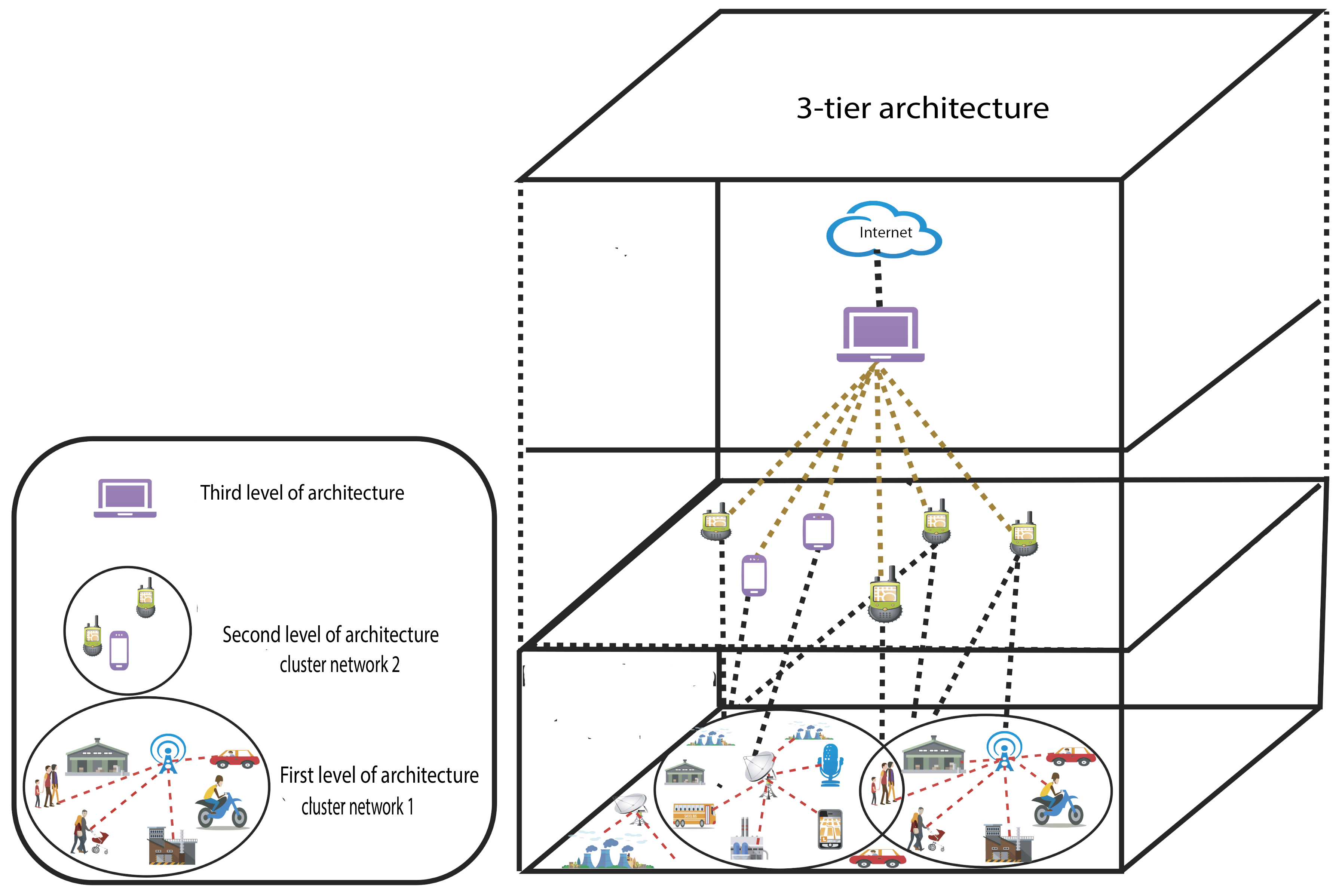
In the context of our study, where the LS-WSN we propose will be dedicated to the collection of big data from intelligent cities, the challenge that drives us is to propose a network that will be able to operate as long as possible without any external intervention related to the energy resource and ensuring maximum coverage of the area of interest. On the other hand, data collection must be relevant and not redundant. We believe that a three-tier LS-WSN architecture coupled with inter-cluster and extra-cluster switching modeling would be better suited to meet the application challenges mentioned above. The data from the collection will be processed to improve or support the activities and services that smart cities offer. In the following section, details our proposal for a three-tier architecture whose particularity is the formation of clusters in the first two levels.

3. Three-Tier Architecture of Ls-Wsns

This section presents our three-tier architecture dedicated to LS-WSN for the collection of big data at the scale of smart cities. A detailed description of our LS-WSN model is presented in Section 3.1. Then we propose to model the inter and extra cluster communication mechanism of the whole network in Section 3.2.

3.1. Architecture Description

Figure 3 presents our proposed heterogeneous LS-WSN architecture model. The peculiarity of the three-tier architecture that we propose compared to those already existing in the literature [33,34], is that the first two levels of the architecture are built on a set of clusters with a well-defined communication strategy.

3.1.1. The Level 1 Network

The first level of our architecture consists of tens of thousands of sensors dedicated to the collection of heterogeneous data. These sensors are to be deployed over a large area on the scale of an intelligent city. Thus, the sensors will be embarked on people, buildings, cars and other related objects in order to collect data of all kinds. With regard to the area of interest, we have chosen to organize the sensors in clusters.

Let us note that at this stage, for a given cluster, the network implements two basic functionalities associated with the sensors: the data collecting sensors in charge of collecting and then transferring data, which we denote $\mathrm{N}1$, and the cluster head denoted CH, which is in charge of the first level of data aggregation. In addition, it should be noted that some $\mathrm{N}1$ type sensors can be mobile. This is due to the fact that the sensors are also embarked on mobile persons and objects. This mobility affects the clusters for which an update procedure is triggered periodically for better monitoring.

3.1.2. The Level 2 Network

Built on a set of sensors of a different type than those of level 1, the level 2 network is in charge of collecting big data of environmental type. However, the number of sensors deployed is relatively lower than that of the level 1 network. The sensors of this network are also organized in clusters. In addition to collecting environmental data, these sensors also serve as relays for the transfer of data collected by the level 1 network to the BS. The layer 2 network is stationary and is rated $\mathrm{N}2$.

Compared to level 1 sensors, sensors at this level perform increasingly complex tasks. They collect environmental data (presence, ${\mathrm{CO}}_2$ detector, smoke detector, humidity, etc.) and relay this data including medical data to the BS. Environmental sensors have processing and aggregation capability. At the scale of a city, the deployment of environmental sensors must be optimized to cover the entire area of interest (camera field of view) and to provide better connectivity with the sink (radio range).

3.1.3. The Level 3 Network

The last level of our architecture consists only of the well. The latter is the destination of the data collected in the two previous levels. The well is the central node of the network, it has complete knowledge of the functioning of the other two levels. Its main functionality is the reception and processing of information from the sensors. It ensures a good adjustment and control of the nodes of the lower levels.

Compared to existing architecture models, our model has the advantage of providing two levels of data management and access (distributed storage): local access on the CH (which can be a PDA for instance) and remote access on the central sink node (linked to a computer). This will significantly reduce redundancy in the big data collected in general. This reduction in redundancy translates into lower power consumption and data processing loads at the sensor and network level, implying low consumption of the overall network. Indeed, multi-hop transfer and adjustment of the power emitted by the sensors offer the advantage of minimizing energy and interference with other nodes (collisions and retransmissions).

3.2. Implementation of the Architecture

The heuristics and construction algorithms of the different clusters of our architecture are taken from the work of Kone et al. [35]. We are interested here in the behaviors of the different sensors of the network as well as in the arrangement of the tasks that can allow us to save the energy of the sensors and to maximize the life span of the network. It should be noted that sensors are generally not autonomous in terms of energy, they are powered by external energy sources such as a battery, for example, the exhaustion of the battery puts the sensor out of use and disconnects it from the network. The problem of the lifespan of the sensors, and therefore that of the network, is closely linked to energy management. Our architecture model relies on the logical structuring of the sensors and the management of the radio component in order to maximize the life of the network.

Indeed, considering the low energy autonomy that characterizes sensors in general and those of level 1 in particular, we propose a heuristic based on the management of the radio component of the sensors to reduce the energy consumption. To do so, we opt for an adjustment of the periods of activity and inactivity (sleep) of the sensors. The sensors must obey the principle of event-driven transmission as shown in Figure 4 as well as the interactions between the different levels, the exchange of wake-up messages between “predecessor” and “successor” nodes in the communication chain. In order to respond to alarms that may be triggered, it is intended that nodes (CH), (N2), and (P) remain in listening mode, and upon receipt of wake-up messages, they must perform the programmed tasks without any restrictions.

With regard to data detection and transmission, interference due to the presence of walls and obstacles may influence the quality of data transmission. In addition, the quality of processing depends on several factors such as: the type of processor, memory, the robustness of the calculation algorithms, the ability to process multimedia content, etc. Finally, the transfer periodicity (transmission interval) of the sensors deployed at the first level of the architecture (N1) can also have an impact on its energy consumption at the sensor level. These aspects will be demonstrated in the simulation part.

The communication arrangement heuristic is done in two phases: the modeling of the communication within a level and the modeling of the communication between the different levels of the model. In both cases, we will use a states-transitions diagram to describe the behavior associated with the different sensors and the programming of the tasks to be executed according to the realization of the application scenario. The second phase is the definition of inter-sensor communications (inter-level interactions).

4. Communication Architecture

4.1. Modeling of Intra-Level Communication Architecture

The functioning of our architecture can be modeled through a set of State-Transition diagrams. We define the behavior diagram of all the sensors used in the architecture. The behavior of the different sensors depends largely on their nature, their expected functionalities and their positions. It should be remembered that depending on the architecture, the sensors deployed at the first level have no predecessor. Similarly, the well has no successor. We model in the following the functional states as well as the possible transitions for the different behaviors of each sensor that can induce a change in the global behavior of the network.

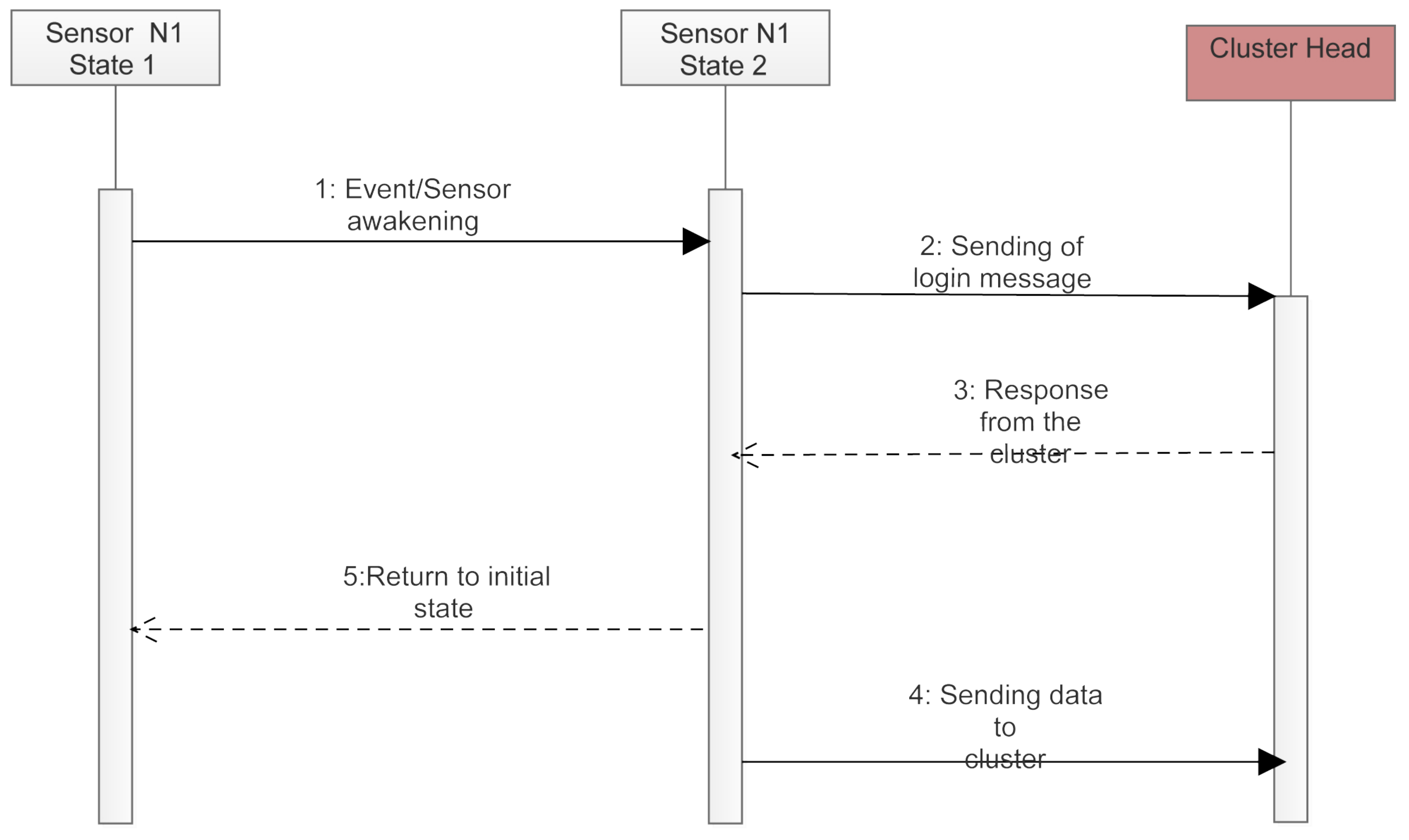
4.1.1. Level 1 Sensors

The main task assigned to sensors at this level is the detection and subsequent collection of man-made big data and related activities. At this stage, the sensors are not involved in packet routing. Each data collected by a sensor is routed to its CH through a communication with one or more hops depending on the position of the sensor. The behavior of each sensor at this level is modeled according to three states as shown in the Figure 5.

In state 1, the radio module of each sensor remains dyed, however, the sensors continuously monitor and control the man and his related activities (the acquisition unit of the sensors remains permanently active allowing the node to send alert messages, thus minimizing the delay, as well as periodically sending the collected measurements). The sensors switch to state 2 when their sleep period has expired or if an event occurs. In this state, each sensor monitors and then collects data, in order to transfer the data to the CH. It sends a message (a request to send data) to its CH and waits (according to a defined time delay) for a response (state 3). If the message is not received, it retransmits the message. At this stage, a selective retransmission mechanism (allowing the selection of the quantities to be retransmitted) must be considered taking into account the fixed number of retransmissions (according to the priority of the captured quantity). When the data transfer request is approved by the CH, the sensor transfers the collected data to its CH and returns to the sleep state (state 1), its radio is therefore switched off. This state 1 represents the stage of the energy conservation phase of the sensors (sleep during periods of inactivity).

4.1.2. Cluster Head

Cluster heads (CHs) are intelligent sensors with more power and energy capacity, responsible for the clusters formed by the level 1 (N1) sensors. They have a data aggregation capacity, which allows them to propose a first level of aggregation of received data. The CHs manage the connection between the level 1 network and the level 2 network. The data received by the CH is analyzed by the latter in order to propose an appropriate routing (level 2 or sink sensors). Four states are used to model the behavior of the CH as shown in the Figure 6.

In state 1, the CHs are waiting for sensor data. If they receive a message, a transition to state 2 takes place. In this state, they analyze the received msg, add their own information and route it to the well. Several cases can be considered to select an appropriate route (destination address). For example, if a data requires a short delay and a high priority, the CH first tries to reach the well directly (sending an MSG with the well address). If the MSG-ACK is not received, they try to send the message to a level 2 sensor indicating the importance of the data in order to adapt the parameters: selection of the type of content to be transmitted, relay of the collected data, and/or transmission of the images to remove the doubt in the case of an abnormal situation. In state 4, they wait for the msg-ok from the level 2 sensor. If the msg-ok is not received it returns to state 2, otherwise they return to the initial state 1. We note that in states 3 and 4, a selective retransmission mechanism is required to avoid infinite cycling (defined delay and/or limitation of the number of retransmissions).

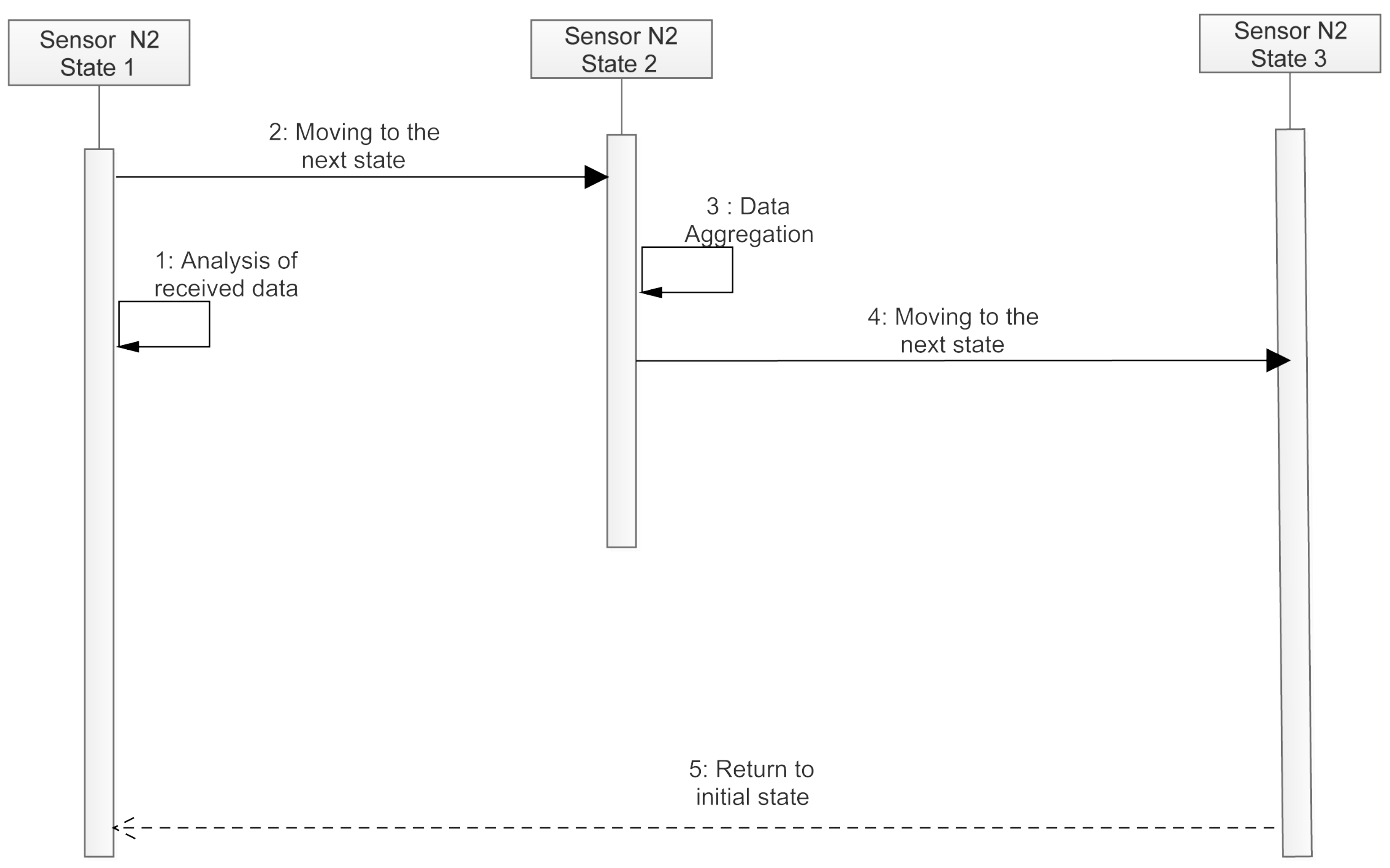
4.1.3. Level 2 Sensor

The second level of our architecture consists of multimedia sensors. They are in charge of collecting multimedia data (camera, sound, video) throughout the intelligent city, but they also serve as gateways for the transfer of data from level 1. To minimize delay and respond to alerts, the radio component of these sensors must remain on standby for wake-up messages. During the monitoring phase, the Level 2 sensors can determine the type of data to be transferred. To do this we suggest that they analyze the msg messages received from the CHs in order to decide whether to activate the camera’s sensor card, collect environmental data or relay only level 1 data. From an energy point of view, it does not seem desirable at this stage to permanently activate the camera’s sensor card. Figure 7 summarizes the modeling of the behavior of level 2 sensors (case of sending an msg message if a person is detected).

The activity of sensors 2 turns around the multi-stream transfer of data to level 3 (transfer of single data and/or multimedia content). When a message is received from a CH, the level 2 sensor switches to state 2 and checks the detection of movements in its field of vision (recognition by a presence sensor integrated in the Imote2). If data from level 1 is received, the level 2 sensor switches to state 3 and adds its own information (merged with the data received from the CH) and transmits it (e.g., takes a picture) to the sink. If no data is received after a defined delay, it returns to state 1. One of the advantages of the layer 2 network is that the sensors provide auxiliary (safety) routes to reach the sink.

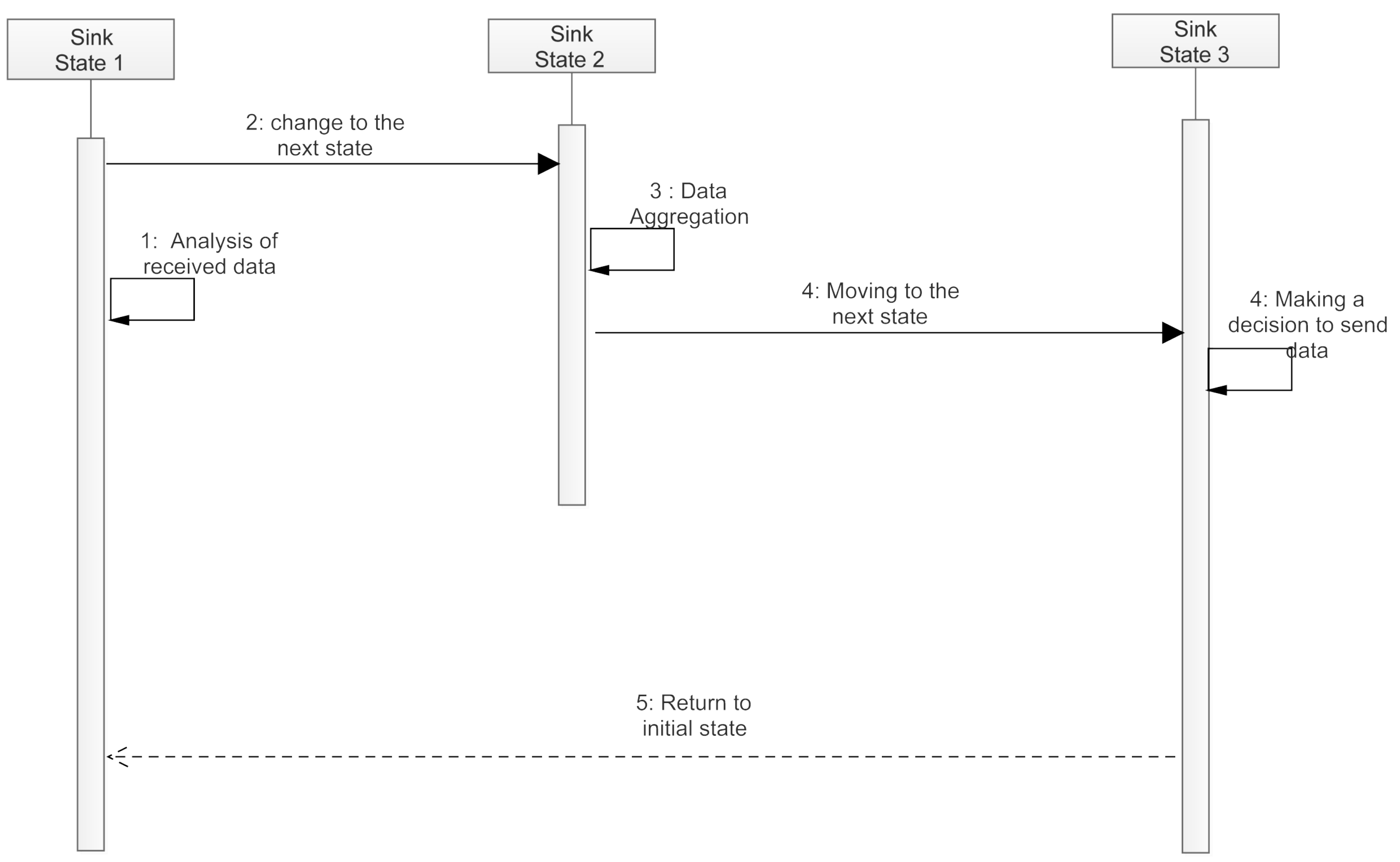
4.1.4. Sink

The sink performs a second level of data aggregation (before the data leaves the WSN home automation network). As described in Figure 8. In state 1, the sink is waiting for a wake-up message from its predecessors on the lower levels (Coordinator or Beacon node). When it receives data, state 2 is activated. In this state, it sends the appropriate acknowledgments (msg-ok), and state 3 for alarm management takes place. At this stage, the sink node makes the decision whether or not to send the received data (e.g., alarms) via external communication systems to the monitoring center (hospital, doctors, etc.). Depending on the selection, either state 4 or state 1 takes place. An important detail must be mentioned for level 2 sensors and the sink: the msg-ok expectation is not shown in the state-transition diagram. We assume that acknowledgments for data and wake-up messages are built into the model.

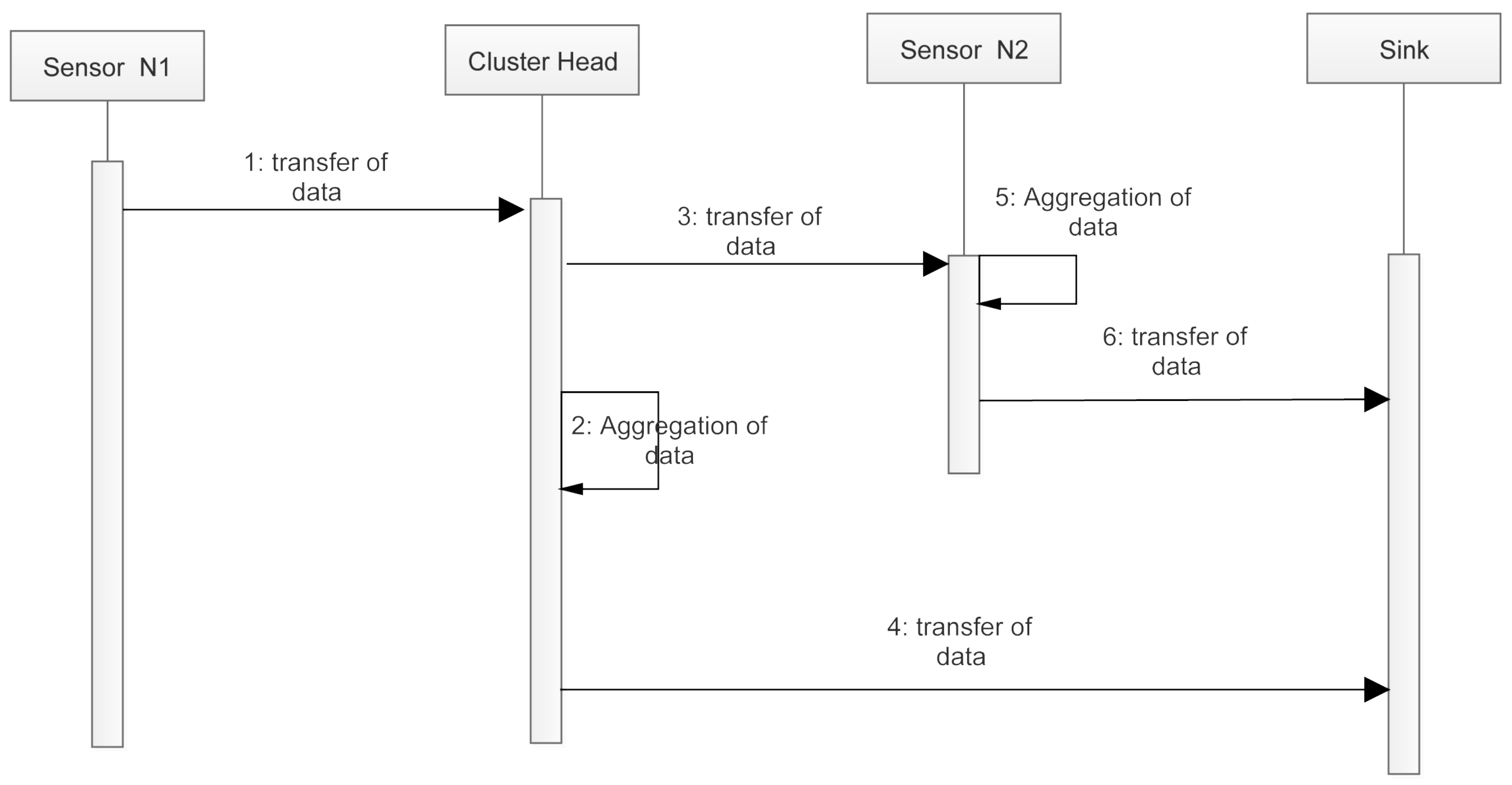
4.2. Modeling the Architecture of Inter-Level Communication

Overall, the different types of sensors in architecture must be organized to collect the big data generated in a smart city. To do this, the three levels of architecture interact by sending a permanent message. As described above, some sensors cannot start their activities before their predecessor completes its task (except for level 1 sensors that have no predecessor in the transmission chain and those initiate communications in our scenario). At the beginning of the deployment, the sensors are activated simultaneously and begin their initialization phase with mutual recognition in order to have a comprehensive view of the network. The level 1 sensors, CHs, level 2 sensors, and the Sink switch off their components except for the transceiver and MCU which remain active (the sensor unit remains inactive) waiting for wake-up messages to be initiated by the level 1 sensor nodes (periodic sending of data/alert messages). The level 1 sensor monitor people and their related activities and react if specific events occur (high or low temperature, abnormal pulse, drop, etc.) and transmit the data via the CHs to the level 2 network.

Environmental data are collected at level 2. In addition, data received from level 1 are also collected. Level 2 consolidates the data and then transfers the data to level 3. To reduce energy consumption, collisions and retransmissions, we propose to adjust the transmission power of the level 1 sensor nodes and the CH so that they only reach the neighboring level 2 sensors.

4.3. Network Energy Consumption Model

We consider our LS-WSN architecture to be made up of N sensors generating periodic and constant size traffic. Each period, each sensor generates an m-bit size message to the sink. The sensors have a limited common transmission range (R), they can be solicited for routing messages from neighboring sensors. Only sensors located at a distance less than R can communicate directly with the sink. Therefore, sensors positioned at a distance of $d\in 2[ktimesR;(k+1\left)timesR\right]$ must use a path of at least k jumps to route messages to the sink.

We then defined a circular geographic model based on the different levels of our architecture. We partitioned the different levels of our architecture into eccentric rings centered on the position of the CH. Each crown has R as width and models one level of the routing tree. We call each crown, level. Let L be the number of levels in the network and $l_0$ the level of the sink. A sensor positioned at the first level of the architecture, furthest from the sink ($l_L$) will be responsible for collecting its own data and will generally not be asked to transmit data from other sensors. A sensor positioned at the second level of the architecture $l_{L-1}$ will have to collect its own data, receive data from some sensors at the lower level $l_L$, and retransmit it to the next hop.

Based on this finding, we consider the energy dissipated for each data sending or receiving operation and give an estimate of the overall energy dissipated by a level taking into account the number of transmitting or receiving operations performed by its sensors. It is important to stress that we do not pretend to calculate the energy consumed with accuracy but we present a possible approximate case with the aim of better distributing the energy consumption in a network of sensors. Moreover, adopting the energy dissipation model of Heinzelman et al. [36] and considering our assumptions, we assume that all sensors dissipate the same amount of energy for a basic operation, either receiving or transmitting. We note, respectively, by $T_x$ and $R_x$, the energy dissipated by a sensor for sending data and receiving data.

Let $n_i$ be the number of sensors in $l_i$ and $E_{l_i}$ the total energy dissipated in $l_i$. Each $n\in l_j$, with $j<L$, is responsible for collecting data in its environment, receiving and transmitting all data received from the sensors in the higher $l_i$ level with $i>j$. According to the same principle, we give the general formula for the total energy consumed by a $l_i$ level in Equation (3).

$$E_{l_i}=(n_i+\cdots +n_L)\times T_x+(n_{i+1}+\cdots +n_L)\times R_x$$

(1)

This leads to:

$$E_{l_i}=T_x\times \sum _{i=j}^L{n}_i+R_x\times \sum _{j=i+1}^L{n}_i$$

(2)

And finally:

$$E_{l_i}=[(T_x+R_x)\times \sum _{j=i+1}^L{n}_i]+T_x\times n_i$$

(3)

5. Results and Discussions

In this section, we examine the results of simulating the implementation of our three-tier architecture and then evaluate its impact on the overall lifetime of the network. For our simulations, we used Omnet++ coupled with the INET framework in order to better adapt the requirements of our study to the big data collection scenario.

Furthermore, in order to evaluate the energy consumption of the LS-WSN deployed in our three-tier architecture, we compared our proposal to other LS-WSN architectures proposed in [37]: “Homogeneous network” and “Hierarchical heterogeneous network”, which are LS-WSN architectures with respectively one and several capture levels. Routing protocols SEP (Stable Election Protocol) [38] and LEACH (Low Energy Adaptive Clustering Hierarchy) [39] were used to simulate the data collection scenario. The parameters used for this purpose are shown in

Table 1. Simulation parameters.

Parameters	Value
Number of levels	3
Maximum sensor range	110
Dimension de la surface	10,000 m × 10,000 m
Duration of simulations (in rounds)	1800
Initial sensor energy	0,8 joules
Transmission energy	$5\times {10}^{-8}$ joules
Energy of receptions	$5\times {10}^{-8}$ joules

.

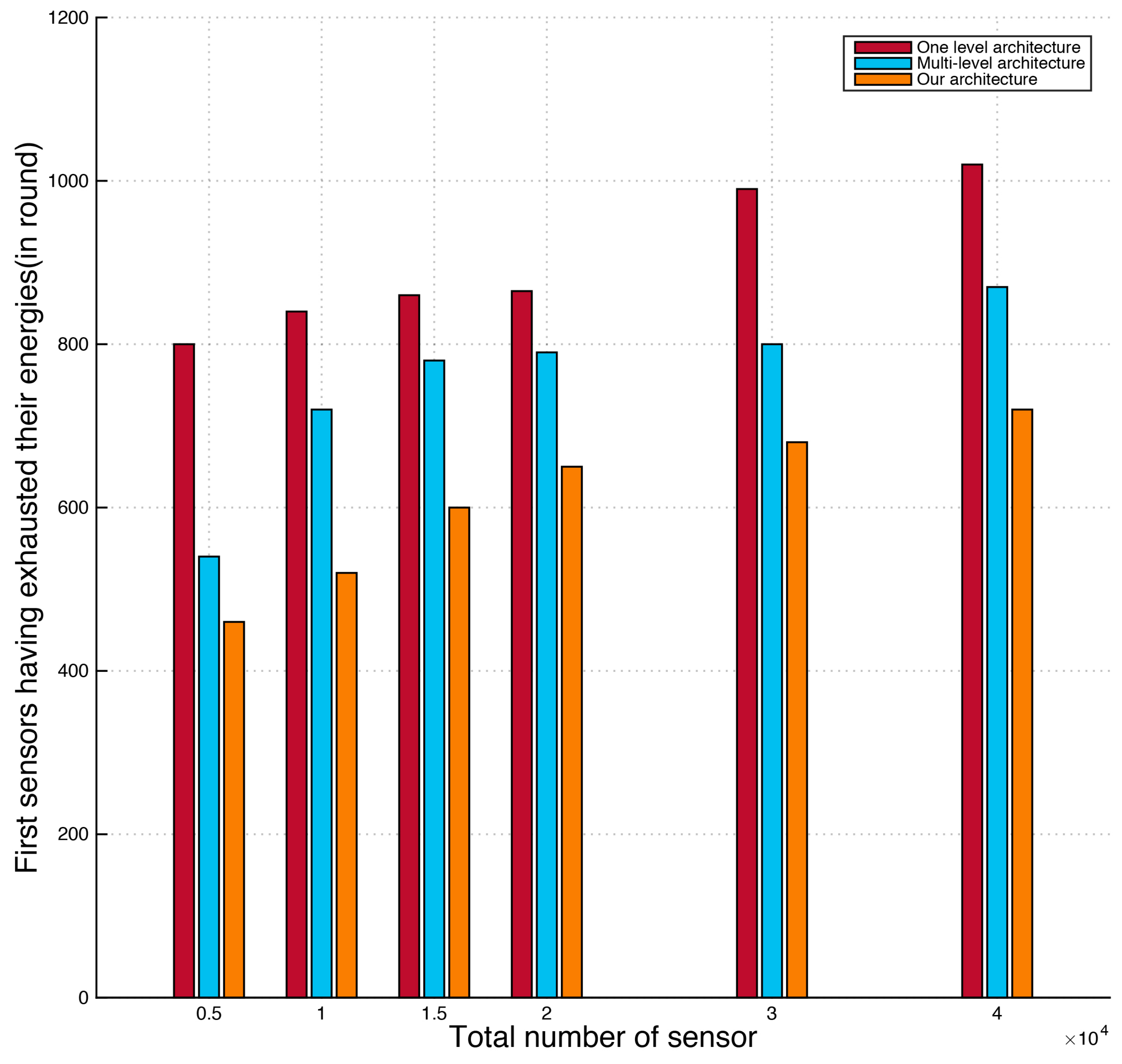
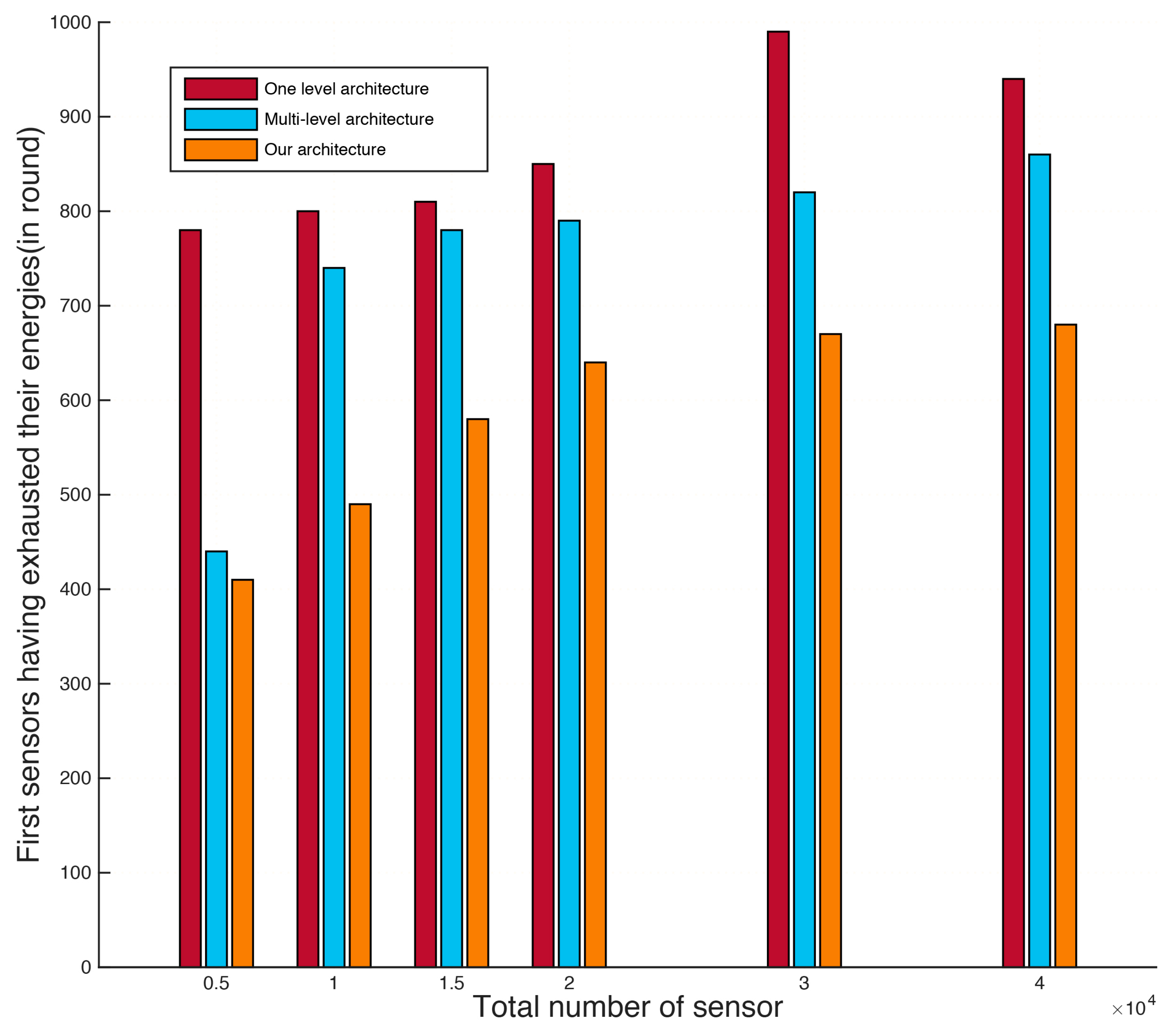
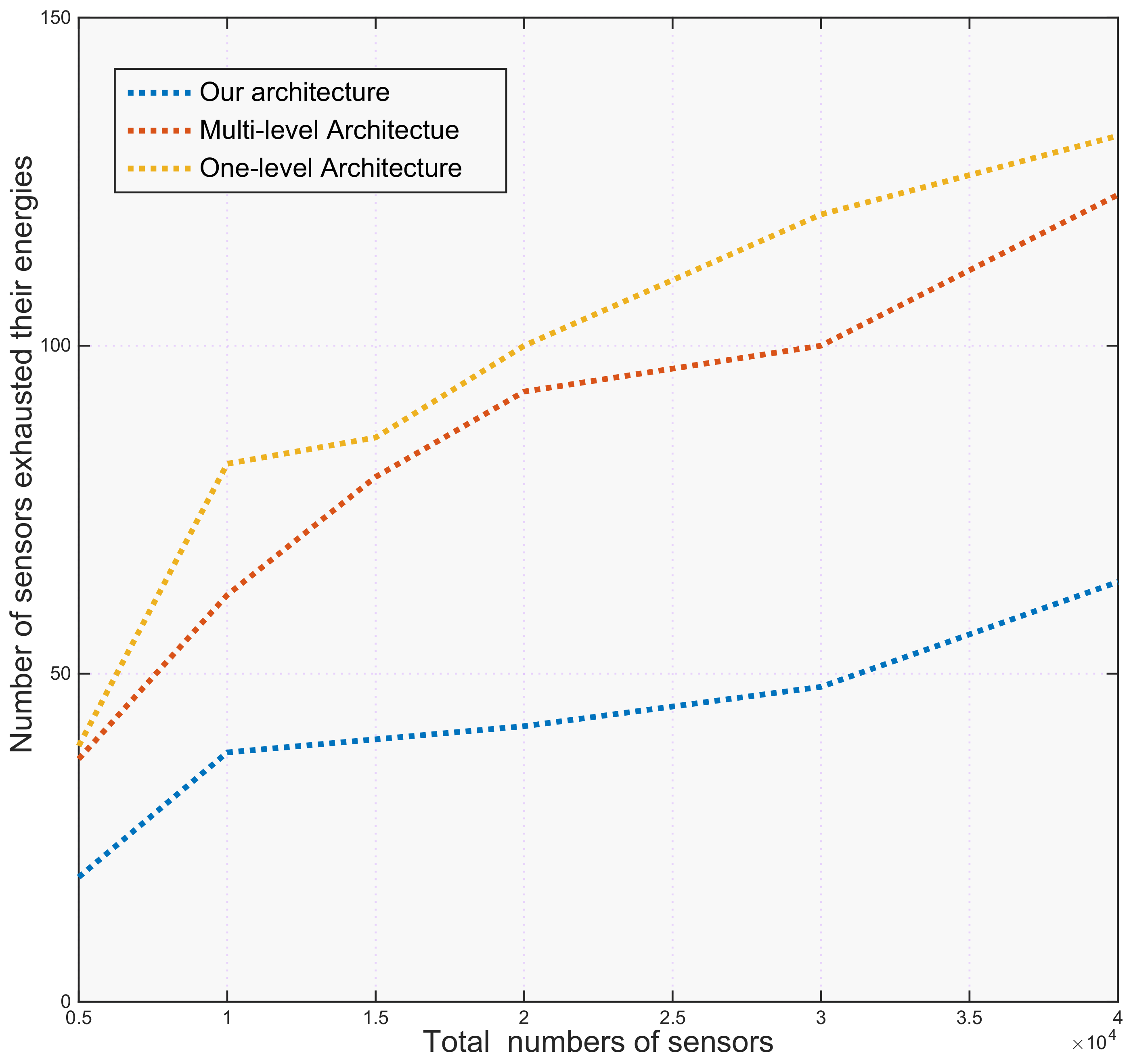
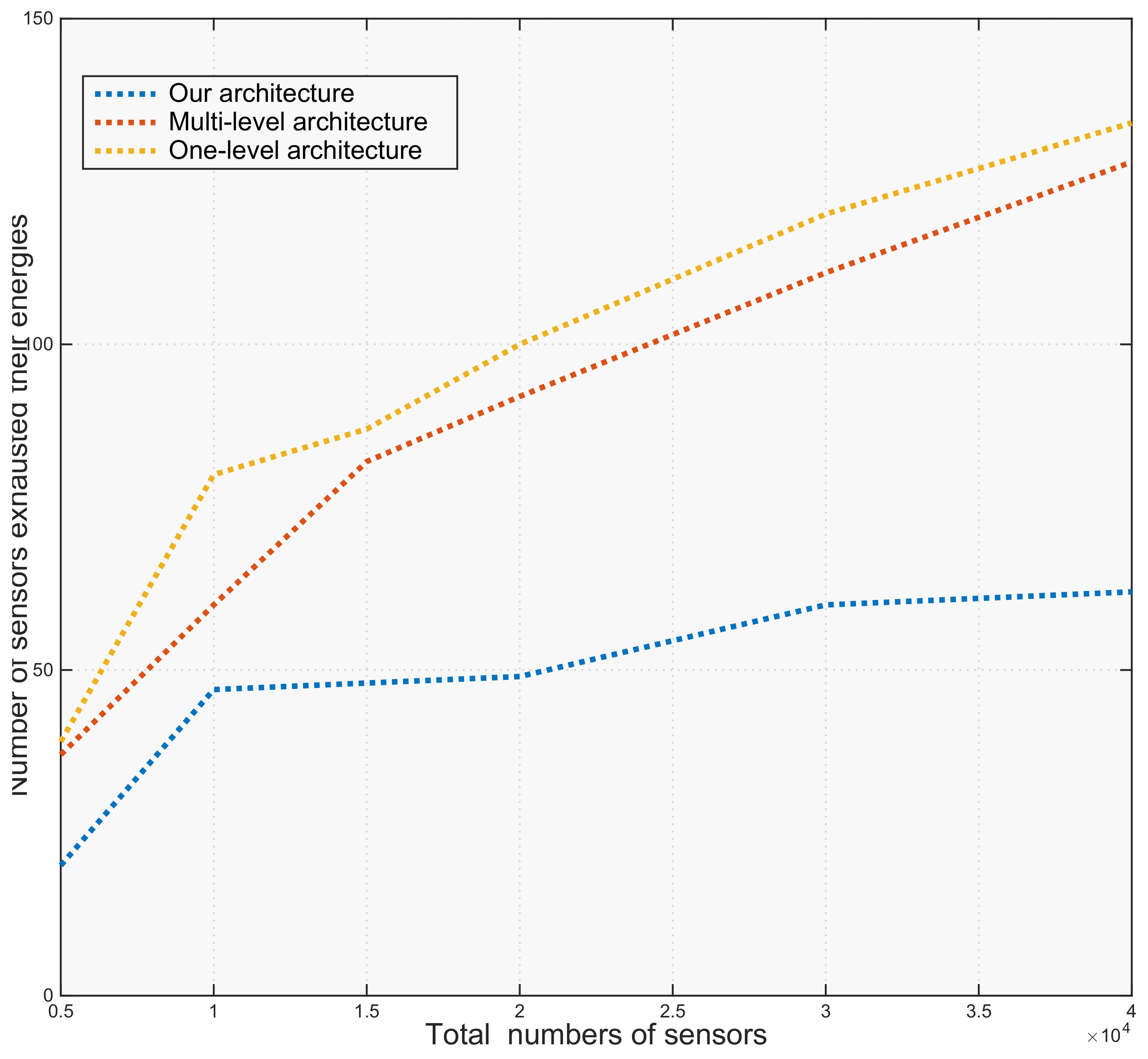
An evaluation of the performance of these different architectures proved the superiority of the proposed three-tier architecture over the other two architectures. 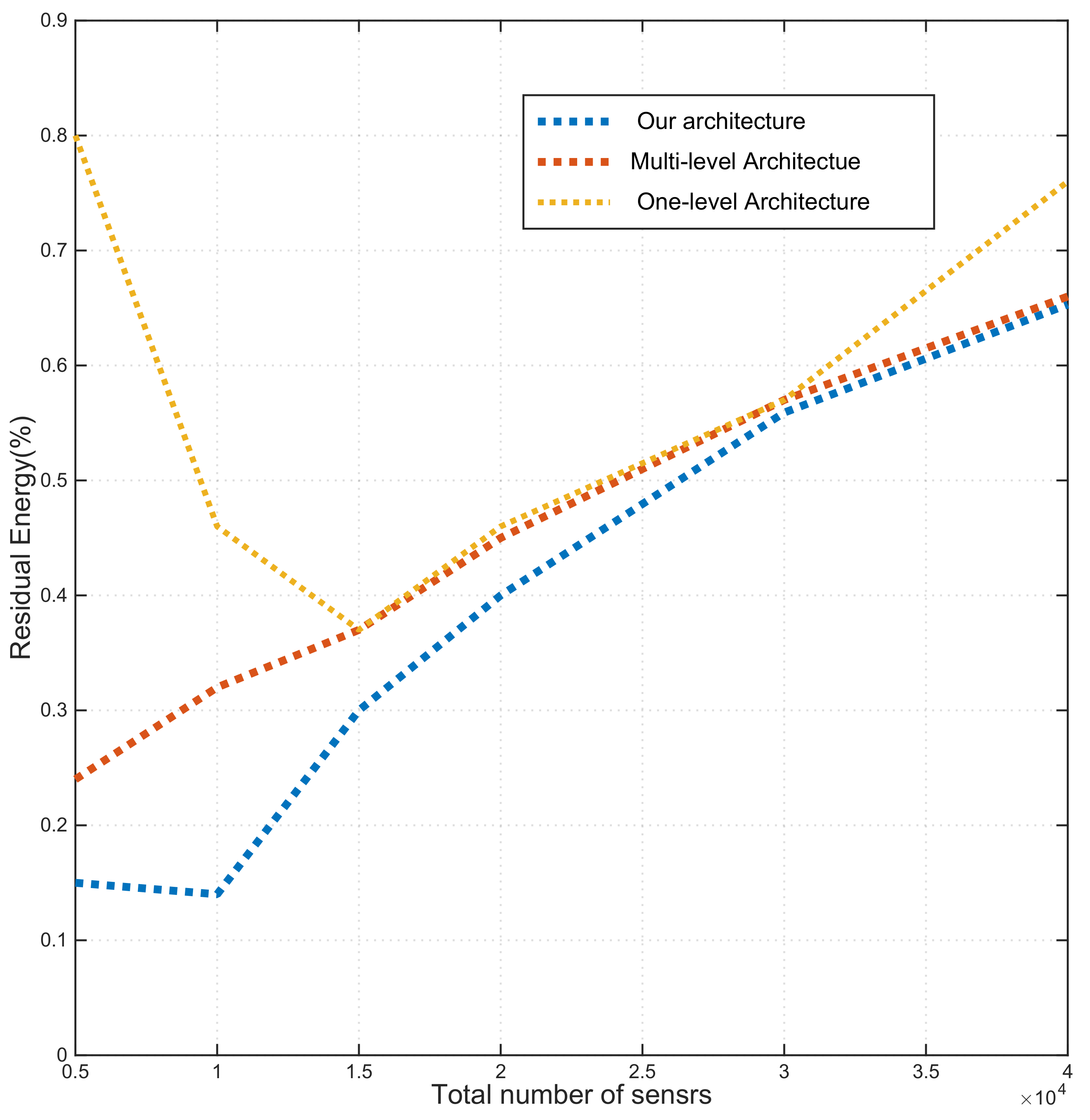This superiority is characterized by a longer network lifetime in terms of the instant of exhaustion of the battery of the first sensor (Figure 9 and Figure 10), in terms of the number of sensors having exhausted all their energy (Figure 11 and Figure 12) and in terms of average residual energy (Figure 13 and Figure 14).

Particularly, Figure 9 and Figure 10 assess the energy consumption of our architecture compared to two other architectures proposed according to two routing protocols namely SEP (Figure 9) and LEACH (Figure 10). The two figures show for each architecture, depending on the number of sensors deployed, when the energy depletion of the sensors occurs. This time is expressed in number of laps.

Our experiments have shown that our three-tier architecture provides a gain in terms of improvement in topology and energy conservation compared to these two other architectures. Then, through another series of simulations, we sought to highlight the importance of the data transmission periods (time intervals) to the well in the energy conservation strategy in the different levels of our architecture.

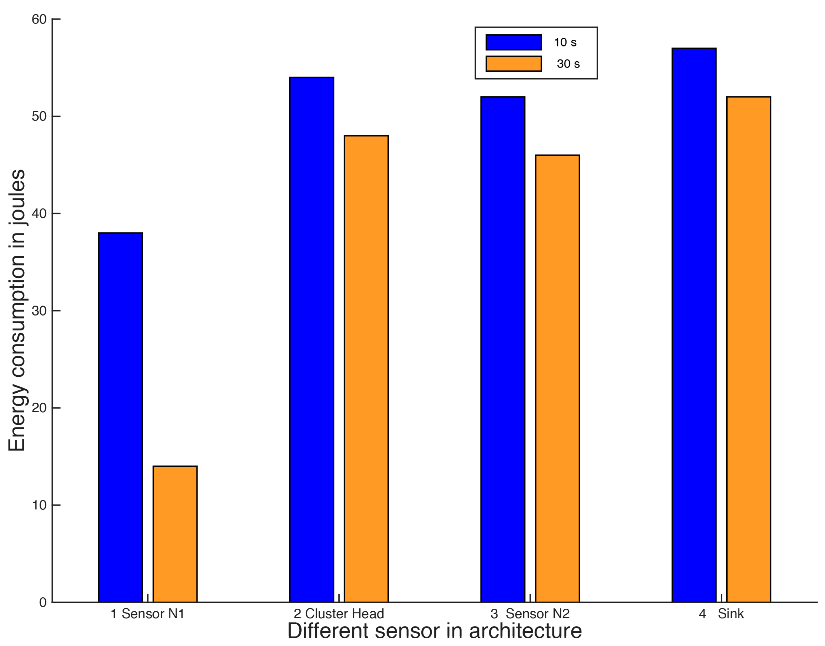
Figure 15 shows the average energy consumption (in Joule) of the sensors of the three levels of the architecture as a function of the transmission time (at a constant step of 10 s). Obviously, energy consumption varies according to the nature and types of sensors. We can clearly see that the well is the type of sensor that is gluttonous for energy: 0.36% of the well’s energy is consumed for a transmission time interval of 10 s (compared to the initial energy of 16200 Joules) and 0.34% for the interval of 30 s. The main reason for this consumption is the well’s operating mode. Due to its nature, the well is the sensor of the model whose radio component must remain in reception mode as long as possible in relation to the sensors (to receive the msg wake-up message). It can also be noted that the consumption of the other sensors (CH), (N1) and (N2) has remained close. The CH consumes 0.33% of its energy for a transmission time interval of 10 s and 0.31% for 30 s, the level 2 sensors consume 0.30% for 10 s and 0.29% for 30 s. Level 1 sensors consume the least amount of energy since 0.24% of energy is consumed for a transmission time interval of 10 s and 0.08% for 30 s. This is due to the fact that level 1 sensors wake up periodically to transfer the collected data to their CH. Confidence intervals in the simulations from Omnet/INET are less than 94.9%.

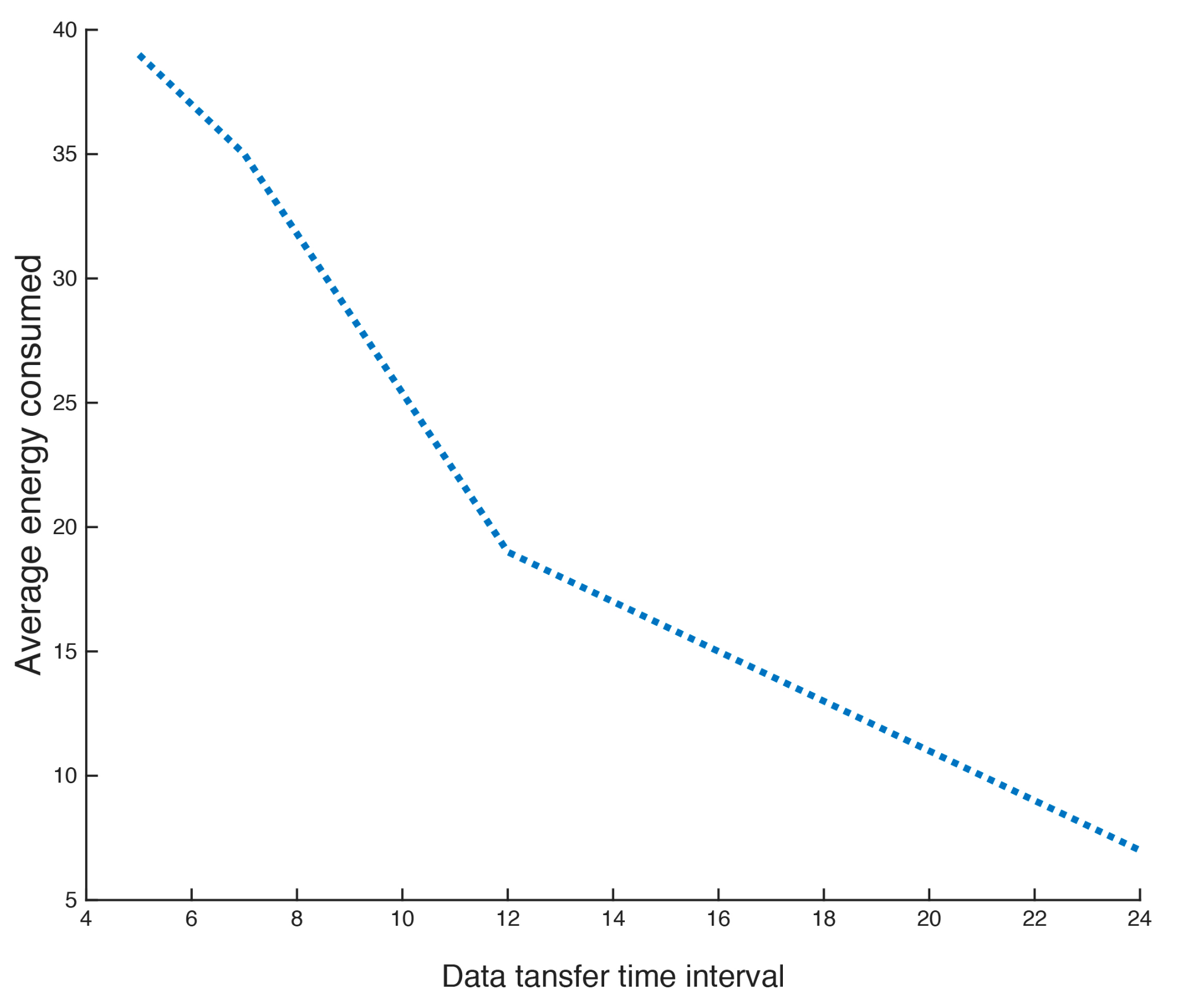
The results of the various simulations show that the data transmission period of the sensors is a significant factor in optimizing the service life of LS-WSNs. This consumption decreases as the data transfer time interval increases, as shown in Figure 16.

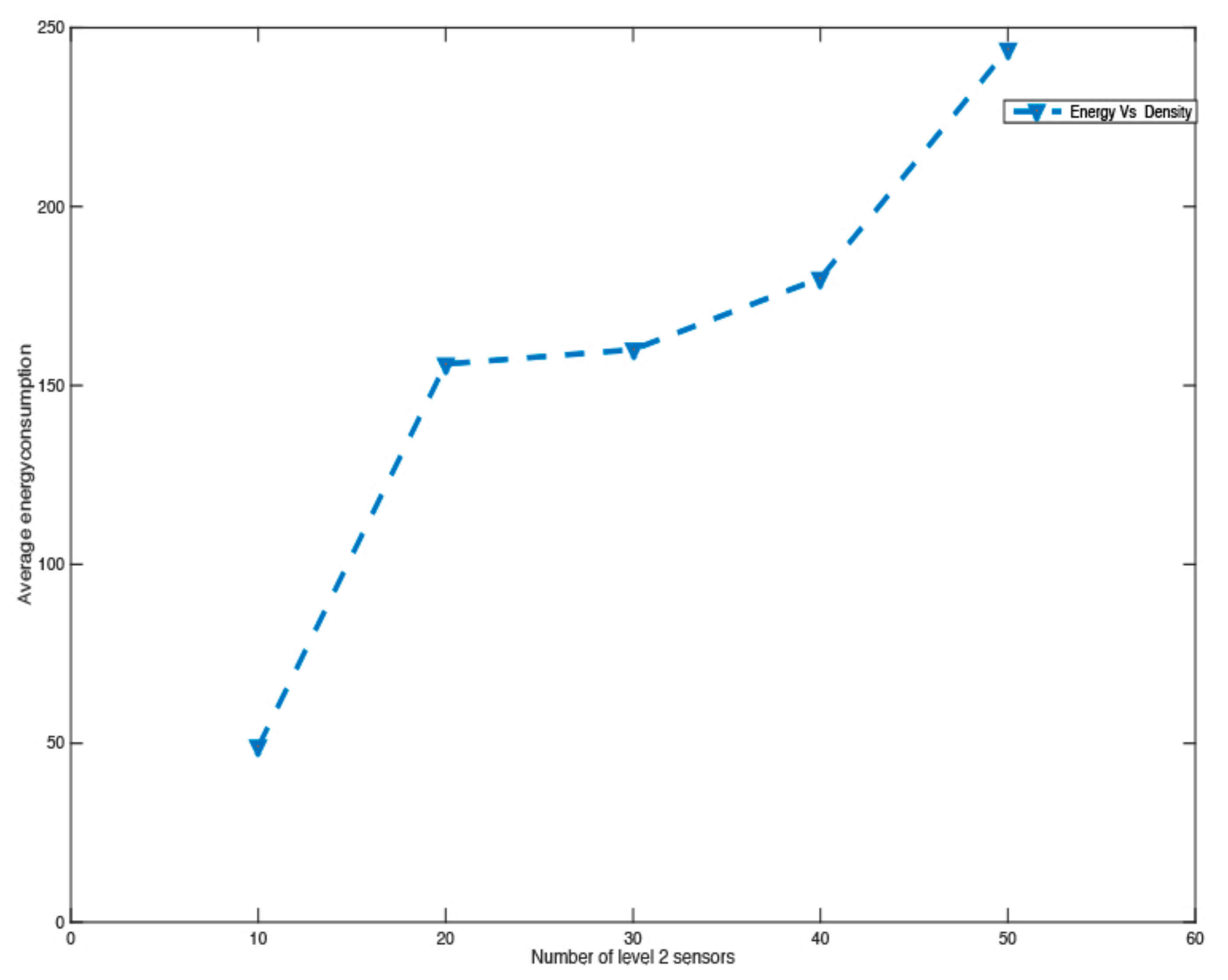
Subsequently, the impact of the network density on the life of the network was studied. Figure 17 shows that the energy consumption of the sensors on the second level of the architecture is dependent on the number of sensors deployed. It is easy to notice through our simulations that the energy consumption of the sensors of this level is proportional to the deployed sensors. These different results show that in addition to the three-tier architecture for LS-WSN deployment, the management of data transmission periods and sensor density contribute well to extending the service life of LS-WSNs.

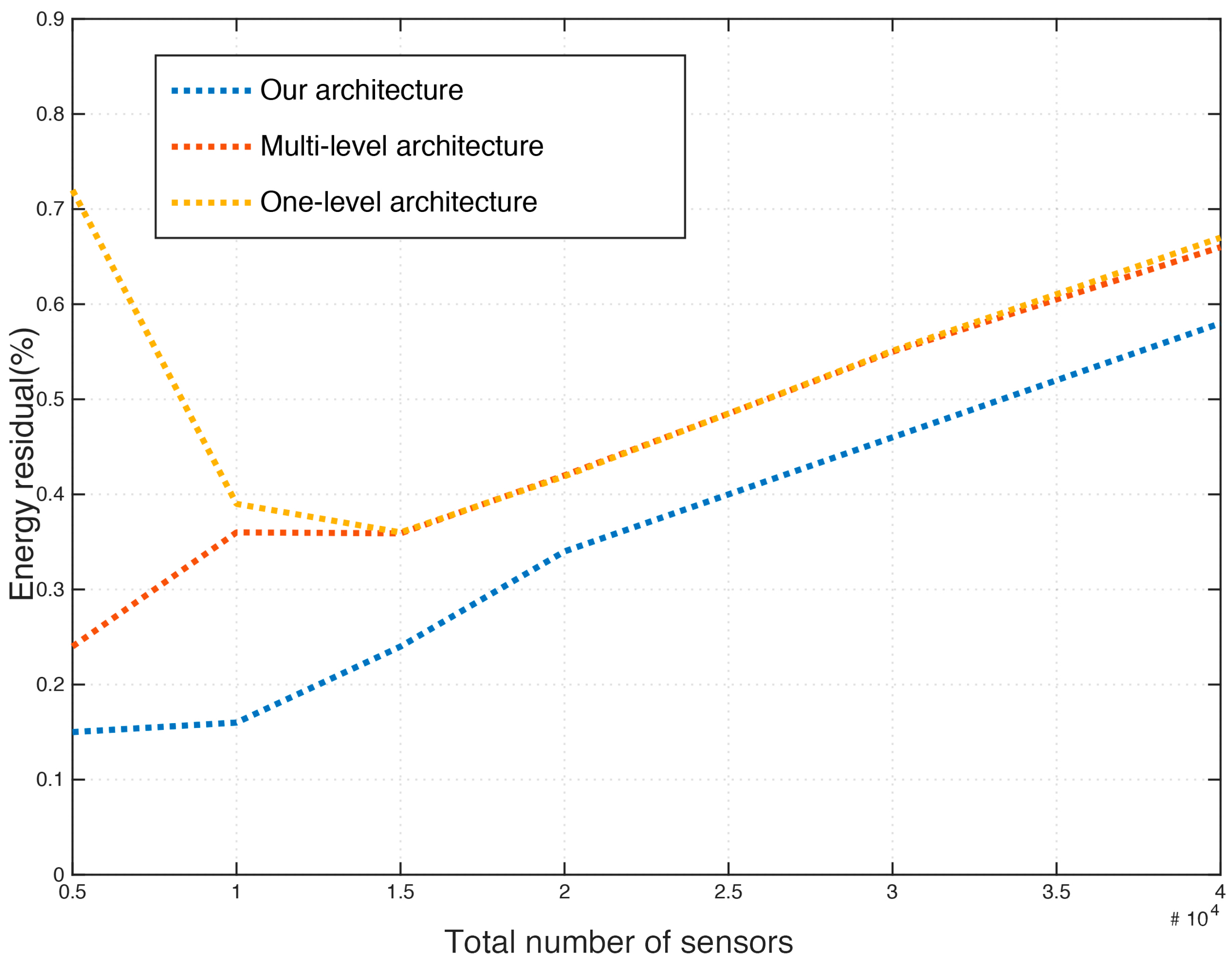
Finally, we evaluated the impact of modeling the tasks of the different sensors across the three levels of the architecture on the energy consumption of the LS-WSN. To do so, we compared our sensor arrangement model with two other models, namely the “Mannasim” model with a single sensor level implemented in the “Homogeneous network” application and the “multi-level” model (MVSN). The different figure highlights the impact of scaling on the average energy consumption of the network. This consumption decreases as the surface area increases (here 15 000 level 2 sensors, transmission interval: 10 s).

We note that the wake-up mechanism that we have implemented in our model through CH, level 2 and Sink sensors allows us to significantly reduce energy consumption by up to two compared to the “single-sensor level” model. However, in the same scenario, our model consumes about 1.7 times more energy than the MVSN network. This result can be explained by the continuous detection implemented in the behavior of the level 1 sensors. Therefore, adjusting the sensing interval could optimize performance.

These results give indications on the impact of the different parameters on the performance of our network, namely: the impact of the nature of the sensors (use of components and energy resources of the sensor groups), the impact of the sensor unit, the impact of the sensor transmission interval (N, N2) and the impact of the scaling.

6. Conclusions

WSNs have become very popular over the past two decades due to the wide range of applications they have enabled. Their autonomy, simplicity of implementation and miniature appearance have made it possible to integrate them into a wide range of small and large-scale applications. The large-scale deployment of sensor networks raises major challenges, which we cite as: (i) ensuring full connectivity and optimal coverage, (ii) ensuring efficient data dissemination, (iii) reducing interference. The ultimate goal for sensor networks is to best conserve sensor energy in order to extend the life of the network. It is within this framework that our main contributions, summarized below, are made. We first proposed various strategies to maximize the lifetime of LS-WSNs. The first solution is a three-tier sensor deployment architecture maximizing the coverage of the area of interest. The second contribution to extend the life of the LS-WSNs was a modeling and arrangement of sensor activities taking into account the location of the sensors in the three tiers of the proposed deployment architecture.

Our contributions have been validated by a series of simulations. The various results have shown that our approach provides better performance that helps maximize the life of the network. These performances are in terms of longer network lifetime in terms of the instant of exhaustion of the battery of the first sensor (Figure 9 and Figure 10), of the number of sensors having totally exhausted their energy (Figure 11 and Figure 12) and in terms of the average residual energy (Figure 13 and Figure 14) of the network. These performances are explained by the intelligent modeling of the sensors’ activity through the three levels of the architecture. We have been able to show that a significant energy gain can be achieved through the formation of clusters across the different levels of the architecture since it allows the organization of sensor activity, maintenance of topology and efficient, fast and inexpensive routing of the collected data.

Our experimental studies have revealed the undeniable contribution that can be made by adopting a three-tier architecture combined with efficient modeling of the tasks of the different sensors in comparison with hierarchical methods without management of sensor activities. On the other hand, intelligent modeling of sensor activity across the three levels of the architecture has shown its great interest in our context of large-scale networks because of the significant energy gain they induce since they are based on simple and local calculations. Finally, we managed to show that a significant energy gain can be achieved through the formation of clusters across the different levels of the architecture since it allows to organize the sensor activities, maintain the topology and allows an efficient, fast and inexpensive routing of the collected data. As future work, we continue to investigate ways to improve the quality of our proposed three-tier architecture. Thus we will seek to optimize the deployment of relay sensors in the clusters formed in the different levels of our architecture.