Can Defect Prediction Be Useful for Coarse-Level Tasks of Software Testing?

Abstract

It is popular to use software defect prediction (SDP) techniques to predict bugs in software in the past 20 years. Before conducting software testing (ST), the result of SDP assists on resource allocation for ST. However, DP usually works on fine-level tasks (or white-box testing) instead of coarse-level tasks (or black-box testing). Before ST or without historical execution information, it is difficult to get resource allocated properly. Therefore, a SDP-based approach, named DPAHM, is proposed to assist on arranging resource for coarse-level tasks. The method combines analytic hierarchy process (AHP) and variant incidence matrix. Besides, we apply the proposed DPAHM into a proprietary software, named MC. Besides, we conduct an up-to-down structure, including three layers for MC. Additionally, the performance measure of each layer is calculated based on the SDP result. Therefore, the resource allocation strategy for coarse-level tasks is gained according to the prediction result. The experiment indicates our proposed method is effective for resource allocation of coarse-level tasks before executing ST.

1. Introduction

Software testing (ST) is an necessary and vital activity in software quality assurance activities [1,2,3]. ST assists in finding defects (aka. bugs) to improve software reliability and quality [3,4,5]. Distributing test resources evenly makes defective and non-defective software entities (such as, class, file, function, subsystem) treated equally, which will lead to a waste of test resources (e.g., time, budget, software testers, etc.) or even do not meet the test objectives, especially with limited resource [6,7]. Therefore, before performing ST, it is quite important to appropriately allocate the resources.

Software defect prediction (SDP), which uses historical defect data including static code metrics (aka. features) and historical defect information (aka. labels) to predict the defect situations of entities via machine learning or deep learning techniques, is a good way to alleviate the issue mentioned above [8,9,10,11,12,13,14,15,16,17,18]. If there is lack of local historical defect data, cross-project defect data can be collected for SDP, named cross-project defect prediction (CPDP) [19,20,21,22,23,24]. However, the granularity of prediction results relies on historical defect data and prediction models. That is, if the defect information is class-level and binary (i.e., the entity is defective or non-defective), only the machine learning algorithms that are able to implement binary classification targets are used to predict the class under test defect or not.

For ST, generally, test methods can be divided into white-box testing (WBT), which focuses on source codes (such as code review, module or unit testing) and black-box testing (BBT), which is related to inputs and outputs of the system without internal structure (such as system testing or functional testing) [25]. We refer WBT and BBT as methods for fine- and coarse-level tasks of ST, respectively. Moreover, researchers or industrial practitioners proposed several approaches to design test cases and improve test quality for the two tasks [3,26,27]. For instance, Mostafa et al. proposed a coverage-based test case prioritization (TCP) method by using the code coverage data of code units and the fault-proneness estimations to prioritize test cases [26]. The authors of Chen et al. combined adaptive random sequence approach with clustering by applying black-box information to make TCP [27]. These authors wanted to refine test cases by using execution information to assist on resource allocation.

From the summary above, SDP can be widely used without execution or code coverage information for fine-level tasks instead of coarse-level test tasks. However, how should managers or project leaders arrange the resources when they face on coarse-level test tasks? Can the defect prediction results provide some meaningful information for coarse-level test tasks?

Based on the above motivation and need, in this study, we consider resource allocation for coarse-level tasks of ST as a single objective decision problem. We proposed a DP-based association hierarchy method (DPAHM) using incidence matrix and analytic hierarchy process (AHP). We conduct hierarchy framework that consists of three layers via AHP and analyze relationships between the inter-level (i.e., coarse- and fine-level) and intro-level (i.e., coarse- or fine-level) via incidence matrix, and then calculate the SDP result of the top-layer from AHP based on the SDP result of the bottom-layer, which also drives from AHP. The SDP result of the top-layer is the strategy for coarse-level test tasks. Besides, our contributions are as follows:

• We apply SDP and make use of the prediction information for coarse-level tasks of ST.
• We combine AHP with incidence matrix to conduct an up-to-down association hierarchy framework.
• We propose a defect prediction based on AHP and incidence matrix, and use an example to apply DPAHM.

Moreover, our study aims at answering the following research questions (RQs):

• RQ1: how is defect prediction used for coarse-level test tasks?
• RQ2: can DPAHM complement different defect prediction task types?
• RQ3: how do different defect prediction learners affect DPAHM?

The remainder of the study is organized, as follows: Section 2 introduces the background and reviews the related work. Section 3 describes our research method: DPAHM. Section 4 uses a project example to verify the effectiveness of our proposed method. Section 5 presents and discusses the experiment results. Section 6 points out the potential threats to validity of our study. Finally, Section 7 concludes this study and states the future work directions.

2. Reviews of Related Works

As is shown in Reviews of Related Works, state-of-art research results about ST, SDP, AHP and incidence matrix are summarized, as follows:

2.1. Software Testing

ST is an effective process in the develop cycle to reduce the defects in software. it can be divided into different ways. According to testing types, software testing includes unit testing, system testing, graphical user interface (GUI) testing, performance testing, user acceptance testing, and other types [3]. ST will be referred to unit testing (aka, module testing), integration testing, function testing, system testing, acceptance testing, and installation testing [25] from the perspective of development processes. According to testing techniques, it can be classified as functional testing, structural testing, and code reading [28]. In addition, WBT and BBT are two common methods of ST [3,25]. The ST process costs around 45% budget of the software develop cost [29]. Therefore, many practitioners or researchers reported approaches to make resource allocation more reasonably.

Several researchers analyzed software to assist on ST [29,30]. For example, Murrill proposed a model, called dynamic error flow analysis (DEFA), about the semantic behavior of a program in fine-level tasks and produced a testing strategy from DEFA analysis [30]. Yumoto et al. proposed a test analysis method for BBT by using a test category and organizing the classification based on fault and application under test knowledge [29].

Several authors proposed TCP methods using white- or black-box information [26,27]. For example, Mostafa et al. improved the coverage-based TCP method by considering the fault-proneness distribution over code units for fine-level tasks [26]. Chi et al. extended the original additional greedy coverage algorithm for TCP called Additional Greedy method Call sequence) by using dynamic relation-based coverage as measurement [31]. Parejo et al. used considered three prioritization objectives for TCP in Highly-Configurable Systems [32]. Chen et al. leveraged black-box related information in order to propose a TCP approach with adaptive random sequence and clustering [27].

Several researchers reported test case selection (TCS) or test case minimization (TCM) approaches, such as literature [33,34,35]. Banias took low memory consumption into consideration that is suited for medium to large projects and proposed a dynamic programming approach for TCS issues [33]. Arrieta et al. proposed a cost-effective approach, which defined six effectiveness measures and one cost measure relying on black-box data [34]. Zhang et al. applied the Uncertainty Theory and multi-objective search to test case generation (TCG) and TCM [35].

However, if there does not exist execution information or coverage data, their methods cannot work well for resource allocation.

2.2. Software Defect Prediction

SDP is one of the hottest topics of software engineering in two decades, because of its predictability. Test leaders or managers want to know the defect situation in a software under test (SUT) via SDP techniques before executing ST work. There has been many researchers study on SDP issues to improve prediction performances [5,8,9,10,11,12,13,14,36,37,38]. According to different prediction tasks, SDP can be divided into binary classification tasks (such as [14,37,39,40]), multi-classification tasks (such as, [41,42]), ranking tasks (such as [5,38,43] ), and numeric tasks (such as [44,45,46]).

For the issues in SDP, some research teams focus on handling defect data, such as feature selection [14,47], instance selection [47,48], and class imbalance processing [36,49]. Some groups stated some novel algorithms [36,50,51], such as TCA+ [51], CCA [52], and TNB [50]. Some articles reported different machine learning algorithms and prediction models for binary classification tasks [37,39,40]. Several research scholars used historical numeric defect data to predict the defect numbers of every entity under test [44,45,46]. Additionally, paper [38,43] paid attention to rank software entities to give testers some guidance for resource allocation.

However, these techniques are aiming at predicting defect in fine-level (such as class, function, file) with static code information without execution data. For coarse-level prediction(such as system), SDP seems to be less effective.

2.3. Analytic Hierarchy Process

Analytic hierarchy process (AHP) is a classic hierarchical decision analysis method proposed by Thomas L. Saaty to help decision-makers to quantify qualitative problems [53]. There are three steps of AHP in total. In the first step, a hierarchical structure that contains three different layers (i.e., goal, criteria, and alternatives, respectively) is built. In the second step, the relationships between inter-layers (i.e., alternatives- and goal-layer, criteria-, and alternatives-layer) are determined by judgment matrix and the relative weights are determined. In the third step, the total rank is derived and corresponding consistency is checked. Besides, the final decision of the alternatives is made (see literature [53] for a more detailed description on AHP). AHP is widely used in different areas, such as water quality management [54], safety measures [55], Technology maturity evaluation [56], and space exploration [57].

However, the weight of the AHP method is subjective (see e.g., [55,58]). Therefore, several researchers extend AHP to make the decision more objective. In software engineering, researchers improved AHP for different software objectives. For example, Thapar et al. integrated fuzzy theory with AHP, called FAHP, to measure the reusability of software components [59]. However, the premise of using AHP is that the elements of each layer are independent, which is not always satisfied. In addition to solving the subjectivity of AHP, how to use AHP to clarify the relationship between the elements in each layer is another problem.

2.4. Incidence Matrix

Before summarizing the incidence matrix, we first understand the definitions of graph, undirected or directed graph, and incidence matrix, as shown in Definitions 1–3:

Definition 1 (Graph).

The graph is composed of a finite set of non-empty vertices and a set of edges between vertices, denoted as $G(V,E)$, where

1.

G represents a graph.

2.

V is the set of vertices in graph G (i.e., the vertex set), $V=\{v_1,v_2,\dots ,v_n\}$.

3.

E is the set of edges in graph G (i.e., the edge set), $E=\{e_1,e_2,\dots ,e_m\}$.

Definition 2 (Undirected/Directed graph).

If the graph G that is defined in Definition 1 does not have a directed edge, which means that the edge between the vertices $v_i$ and $v_j$ has no direction, the graph G is called undirected graph. Otherwise, it is called directed graph, whose edge are called directed edge or arc.

1.

An undirected edge is expressed as $(v_i,v_j)$ or $(v_j,v_i)$.

2.

A directed edge is represented by $<v_i,v_j>$, where $v_i$, $v_j$ are called the arc tail and head, respectively.

Definition 3 (Incidence Matrix).

Let arbitrary graph $G(V,E)$, where $h_{ij}$ represents the number of times the vertex $v_i$ is associated with the edge $e_j$. The possible values are 0, 1, 2, …, and the resulting matrix $H\left(G\right)={\left(h_{ij}\right)}_{n\times m}$ is the incidence matrix of graph G.

That is, H is the $n\times m$ incidence matrix, such that

$$h_{ij}=\left\{\begin{array}{c}1,\text{if}{v}_i\text{is}\text{connected}\text{to}{e}_j;\hfill \\ 0,\text{else}.\hfill \end{array}\right.$$

(1)

being $h_{ij}$ the element in the ith row and jth column of matrix H.

Similarly, for directed graph $G^{\prime }$, the element $h_{ij}^{\prime }$ of corresponding incidence matrix $H^{\prime }$ is denoted as

$$h_{ij}^{\prime }=\left\{\begin{array}{c}1,\mathrm{if}{v}_i\text{is}\text{connected}\text{to}\text{the}\text{tail}\text{of}{e}_j;\hfill \\ -1,\text{else}\text{if}{v}_i\text{is}\text{conneted}\text{to}\text{the}\text{head}\text{of}{e}_j;\hfill \\ 0,\text{else}.\hfill \end{array}\right.$$

(2)

being $h_{ij}^{\prime }$ the element in the ith row and jth column of matrix $H^{\prime }$.

Incidence matrix is a graph representation method to represent the relationships between the vertices and edges. Many researchers used the incidence matrix to solve different problems, such as paper [60] for the traffic assignment problem, article [61] for urban development projects evolution, paper [62] for stability analysis of multi-agent systems, and literature [63] for tracing power flow.

In ST, coarse-level tasks need to call many functions or other fine-level units to implement the requirement. Therefore, we only take the positive direction of the directed graph. Because changes of high-level functions do less effect on the low-level functions. For example, a high-level function T calls a low-level function F. When we change the parameters in F, the output from F usually changes, which leads to the change of T. However, if we change the parameters in T that are not related to F, the output result of F will not be affected by T. Thus, in the paper, we define a positive incidence matrix (PIM) $H^{″}$. The related description of is as follows:

Definition 4 (Positive Incidence Matrix).

Let arbitrary graph $G^{″}(V,E)$, where $h_{ij}^{″}$ represents the number of times the vertex $v_i$ is associated with the tail of the edge $e_j$. The possible values are 0, 1, 2, …, and the resulting matrix $H^{″}\left(G\right)={\left(h_{ij}\right)}_{n\times m}^{″}$ is the positive incidence matrix of graph $G^{″}$.

That is, $H^{″}$ is the $n\times m$ positive incidence matrix, such that

$$h_{ij}^{″}=\left\{\begin{array}{c}1,\text{if}{v}_i\text{is}\text{connected}\text{to}\text{the}\text{tail}\text{of}{e}_j;\hfill \\ 0,\text{else}.\hfill \end{array}\right.$$

(3)

being $h_{ij}^{″}$ the element in the ith row and jth column of matrix $H^{″}$.

3. The Association Hierarchy Defect Prediction Method

3.1. Motivation of the Proposed Method

For coarse-level tasks of ST, such as system-level testing, if there are not enough execution information about the fine-level tasks, it is difficult for test leaders or project managers to arrange test resources. Before executing ST, it is more difficult to properly arrange the resource. However, for fine-level tasks, SDP provides a way to predict the defect situation without coverage data or other execution information. It is effective to assist on resource allocation. Besides, effect analysis is a key step for testing. The call relationship between coarse- and fine-level tasks can be gained by analysis.

Therefore, we inspired by AHP and incidence matrix to extend the hierarchy framework. A association hierarchy structure about the whole tasks from up to down is built. Moreover, before executing ST, the defect situation about the coarse-level tasks based on the SDP of fine-level tasks is derived.

3.2. Four Phases of the Proposed Method

The proposed method DPAHM consists of four phases: the framework conduction phase for the whole test tasks, the SDP model conduction phase for the bottom layer, the positive incidence matrix production phase of each part of the framework, and the resource allocation strategy output phase. A brief framework of the entire method is demonstrated, as illustrated in Figure 1. It should be noted that codes, software requirement specifications, and test case specifications are needed. Moreover, the proposed method is applied after code completion and before ST.

Figure 1. A Framework of The Propose Method.

Each stage is summarized, as follows.

In the framework conduction phase, an up-to-down association hierarchy structure about the three different element layers (Goal-, Criteria-, and Alternatives-layers) is conducted. The hierarchy framework is divided according to the vertical call mapping, which is obtained from software requirement specifications. For the Goal-layer, the resource allocation goal is determined by the test manager or project leader according to the requirement specification. The Criteria-layer contains l elements that are numbered from $Criterio{n}_1\left(C1\right)$ to $Criterio{n}_l\left(Cl\right)$. The elements are coarse-level or mixed coarse- and fine-level tasks. Besides, these tasks are obtained from the requirement specification or/and the architecture design specification. In the Alternatives-layer, there are q elements belonging to fine-level tasks are represented by $Alternativ{e}_1$ ($A1$) to $Alternativ{e}_q$ ($Aq$). The Alternatives are derived from specifications, such as the module design specification. In addition, the horizontal relationship between elements is connected according to the horizontal call mapping. The horizontal call mapping is gotten by specifications for coarse-level tasks and obtained by codes for fine-level tasks. That is, according to design specifications for fine- and coarse- tasks, both the horizontal and vertical call relationships can be obtained, and then the association hierarchy structure can be gained.

In the SDP model conduction phase, the SDP model of the bottom layer (i.e., Alternatives-layer) is built, which uses historical defect data from other projects and a machine learning learner $Learner$ in order to train a CPDP model.

In the positive incidence matrix production phase, PIMs from down to up are produced. That is, the vertical PIM about the inter-layer and the horizonal PIM about the intro-layer are produced by regarding the relationships as a directed graph.

In the resource allocation strategy output phase, the prediction result of Criteria-layer (i.e., coarse-level) is calculated by incidence matrix and the fine-level SDP result. Test case specifications is generated according to codes or/and software requirement specifications. Therefore, the allocation resource strategy for coarse-level tasks will be output if the most defective-prone task is predicted according to the prediction result.

Based on these four phases, the prediction order we advise is listed as follows (In the paper, we focus on resource allocation for coarse-level tasks. Thus, it is feasible that all of the prediction results are gained after completing test case specifications for system testing.):

• the prediction result of Alternatives-layer, which should be gained before unit tesing;
• the predction result of Criteria-layer, which should be obtained before system testing (or before integration testing if necessary);
• the resource allocation strategy for coarse-level tasks after completing test case specifications for system testing.

3.3. Implementation Steps of the Proposed Method

According to the framework and four phases mentioned in Section 3.2, there are seven steps in total to complete our approach. Details of each step in the framework are illustrated, as follows. In addition, the relationship between phases and steps is represented in Table 1.

Table 1. The Relationship Between Phases and Steps of Our Proposed Approach.

Phases	Steps
The framework conduction phase	Step 1
The SDP model conduction phase	Step 2
The positive incidence matrix production phase	Step 3 and Step 4
The resource allocation strategy output phase	Step 5, Step 6, and Step 7

• Step 1: determine the goal is making resource allocation for coarse-level tasks and conduct an association hierarchy structure of the ST tasks according to the calling relationship between the outer layer and the inner layer;

  −

  Step 1.1: apply the first step of AHP to build the hierarchy framework of the ST tasks including three layers (Goal-, Criteria-, and Alternatives-layer) from up to down (Note: Criteria-layer can be divided into one or more sublayers.);

  −

  Step 1.2: analyze the relationship between Criteria- or Alternatives-layer, and find the association structure;

• Step 2: conduct a SDP model (In the paper, we conduct a CPDP model for ranking as paper [38] said.) and predict the defect situation for Alternatives-layer;

  −

  Step 2.2: use historical defect training data as $Source$ and a defect learner $learner$ to train a SDP model;

  −

  Step 2.3: apply the $Learner$ to $Target$, which is target project data of Alternatives-layer (i.e., fine-level), to gain the prediction probability vector $p_{alter}$. The formula is as follows:

  $$p_{alter}=Learner(Source,Target)={[p_1,p_2,\cdots ,p_i,\cdots ,p_q]}^T$$

  (4)

  where $p_i$ means the prediction probability of the ith element of Alternatives-layer, q means the length of this layer;

• Step 3: represent the structure of inter- and intro-layers above as directed graphs: $G_{CA}=(V_1,E_1)$, $G_{CC}=(V_2,E_2)$;
• Step 4: gain incidence matrix $H_{ca}$ of inter-layers from $G_{CA}$ and $H_{cc}$ of intro-layers from $G_{CC}$.

  −

  Step 4.1: produce vertical PIM $H_{ca}$ of inter-layers from graph $G_{CA}$ (i.e., Criteria-layer and Alternatives-layer), such that

  $$h_{ca}ij=\left\{\begin{array}{c}\begin{array}{c}\hfill 1,\text{if}\text{the}i\text{th}\text{element}\text{of}\text{Criteria-layer}\text{calls}\text{the}\\ \hfill j\text{th}\text{element}\text{of}\text{Alternatives-layer};\end{array}\hfill \\ 0,\text{else}.\hfill \end{array}\right.$$

  (5)

  being $h_{ca}ij$ the element in the ith row and jth column of matrix $H_{ca}$. Besides, the size of $H_{ca}$ is $l\times q$, where l and q are the number of elements of Criteria- and Alternatives-layer, respectively;

  −

  Step 4.2: obtain horizontal PIM $H_{cc}$ of the Criteria-layer from graph $G_{CC}$. The formula is as follows:

  $$h_{cc}ij=\left\{\begin{array}{c}\begin{array}{c}\hfill 1,\text{if}\text{the}i\text{th}\text{element}\text{calls}\text{the}j\text{th}\text{element}\text{of}\\ \hfill \text{Criteria-layer}\text{or}(i=j);\end{array}\hfill \\ 0,\text{else}.\hfill \end{array}\right.$$

  (6)

  being $h_{cc}ij$ the element in the ith row and jth column of matrix $H_{ca}$. Moreover, the size of $H_{cc}$ is $l\times l$.

• Step 5: calculate the prediction probability vector $p_{cri}$ of Criteria-layer by the following formula:

  $$p_{cri}=H_{l\times l}\times H_{l\times q}\times p_{alter}={[p_1,p_2,\cdots ,p_j,\cdots ,p_l]}^T$$

  (7)

  where $p_j$ denotes the prediction probability of the jth element of Criteria-layer, l means the length of this layer;
• Step 6: normalize the prediction probability vector $p_{cri}$. The formula is illustrated, as follows:

  $$p_{cri}=\frac{p_{cri}-min\left(p_{cri}\right)}{max\left(p_{cri}\right)-min\left(p_{cri}\right)}$$

  (8)

  where $max\left(p_{cri}\right)$ and $min\left(p_{cri}\right)$ are the maximum and minimum value in $p_{cri}$, respectively.
• Step 7: according to the prediction result to arrange the test resource.

4. Case Study

4.1. Research Questions

To verify the effective of our proposed method, three RQs are summarized, as follows.

RQ1: How is SDP used for coarse-level tasks of software testing?

To the best of our knowledge, SDP is widely used for fine-level tasks (i.e., WBT), but is rarely used for coarse-level tasks. Therefore, a basic defect prediction learner $LRMLearner$ is selected for SDP to implement the processes of DPAHM. The question is a complete implementation of the method to show how to use SDP techniques for coarse-level tasks of ST.

RQ2: Can DPAHM complement different defect prediction task types?

The proposed method DPAHM is based on SDP. For different tasks of SDP, the types can be parted into classification, numeric, ranking and so on as Section 2.2 introduced. This question is to explore the prediction granularity-levels of coarse-level task.

RQ3: How do different defect prediction learners affect DPAHM?

Many research indicated that different defect prediction learners make different results for the same datasets [9,38]. This question is to discuss the effect of different learners on DPAHM.

4.2. Experimental Subjects

To answer the three RQs in Section 4.1. We apply our approach to a proprietary software under test. The software named $MC$ is a safety-related electronic system for railway signals, which is completed by the C programming language. $MC$ includes three coarse-level tasks and seventeen fine-level tasks.

For fine-level tasks, there are thirtheen files and four functions. Files are the basic modules which contain a total of 5334 lines of code (LOC). We collected 48 static metrics by LDRA TESTBED, which is an embedded test tool provided by LDRA (https://ldra.com/). Basic information about ID, file name, and some static metrics of $MC$ is illustrated in Table 2. From the table, LOC, McCabe metrics (Cyclomatic Complexity ($vg$), Essential Cyclomatic Complexity ($e\left(vg\right)$ ) ) and Halsteads metrics (Total Operators ($N_1$), Total Operands ($N_2$), Unique Operators(${\eta }_1$), Unique Operands (${\eta }_2$), Length (N), and Volume (V)) are shown. The meaning of McCabe metrics and Halsteads metrics can be referred in paper [64,65], respectively. The basic files are served for four parts (Function 1, Function 2, Function 3, and Function 4) to complete related functions. Table 3 lists the basic descriptive information.

Table 2. The Basic information bout Thirteen Files from Fine-level tasks of MC.

ID	File Name	#Metrics	LOC	$\mathit{vg}$	$\mathit{e}\left(\mathit{vg}\right)$	${\mathit{N}}_1$	${\mathit{N}}_2$	${\mathit{\eta }}_1$	${\mathit{\eta }}_2$	N	V
A1	AD Sample	48	137	6	1	48	67	13	18	115	569
A2	AD Value Acquisition	48	367	1	1	9	47	2	9	56	193
A3	Analog In Press Processing	48	408	6	1	90	130	11	30	220	1178
A4	Analog Condition Calculation	48	1049	29	1	188	524	13	54	712	4319
A5	Rescale Press Value	48	266	3	1	27	41	9	8	68	277
A6	Read BCD ID	48	373	1	1	12	76	1	17	88	366
A7	BCD ID Bit Value Calculation	48	257	2	1	6	5	5	2	11	30
A8	Bogie ID Identification	48	464	5	1	53	173	8	27	226	1159
A9	BCU ID Bit to Byte	48	365	11	1	27	36	7	1	63	189
A10	Car Type Identify	48	298	5	1	7	12	3	1	19	38
A11	Mass Calculation	48	873	49	1	152	326	15	60	478	2977
A12	Mass Valid Arrange	48	290	1	1	10	26	3	9	36	129
A13	Fixed Weight Factor Calculation	48	387	6	1	26	60	11	9	86	371

Table 3. The Basic Information about Four Functions from Fine-level Tasks of MC.

ID	Name	Description
Function1 (F1)	AD calculation Function	Calculate AD value by sampling AD.
Function2 (F2)	Press calculation Function	Calculate the press and rescale the press value.
Function3 (F3)	Read Bogie ID Function	Convert ID bit value to byte, and calculate the Bogie ID.
Function4 (F4)	Mass Weight Calculation Function	When the mass weight signal is valid, Calculate the weight.

Three are three tasks in the coarse level. The names are Stress Calculation Task, Frame Number Acquisition Task, and Frame Number Acquisition Task. These tasks collect voltage signal and mass weight for safety of railway. Moreover, these tasks depend on fine-level tasks. The basic information (such as ID, Description) is presented in Table 4.

Table 4. The Basic Information about Coarse-level Tasks of MC.

ID	Name	Description
Task1 (T1)	Stress Calculation Task	Collect AD current signal and convert the current value to air spring press signal by AD conversion module. The effective range of current signal is 4∼20 mA.
Task2 (T2)	Frame Number Acquisition Task	Collect four channels of AD voltage signal and convert the analog signal through AD conversion module, and determine the car number and bogie ID by the analog signal. The voltage signal that is <2.7 V corresponds to position number 0 and the voltage signal ≥2.7 V corresponds to position number 1.
Task3 (T3)	Mass Weight Calculation Task	Calculate the mass weight by the air spring pressure and the frame information.

4.3. Apply Our Method to MC

4.3.1. The First Phase

According to the test requirement, $MC$ needs to be checked by system testing, integration testing, and unit testing. For coarse-level tasks, the call relationship is derived from development specifications (or documents) and software development engineers. Our goal is to make system testing about three tasks, which is implemented by calling four integration functions. For fine-level tasks, the relationship is gained by the code and specifications. Besides, the functions, which will be tested in the integration testing process, call thirteen files (units), which will be checked by unit testing.

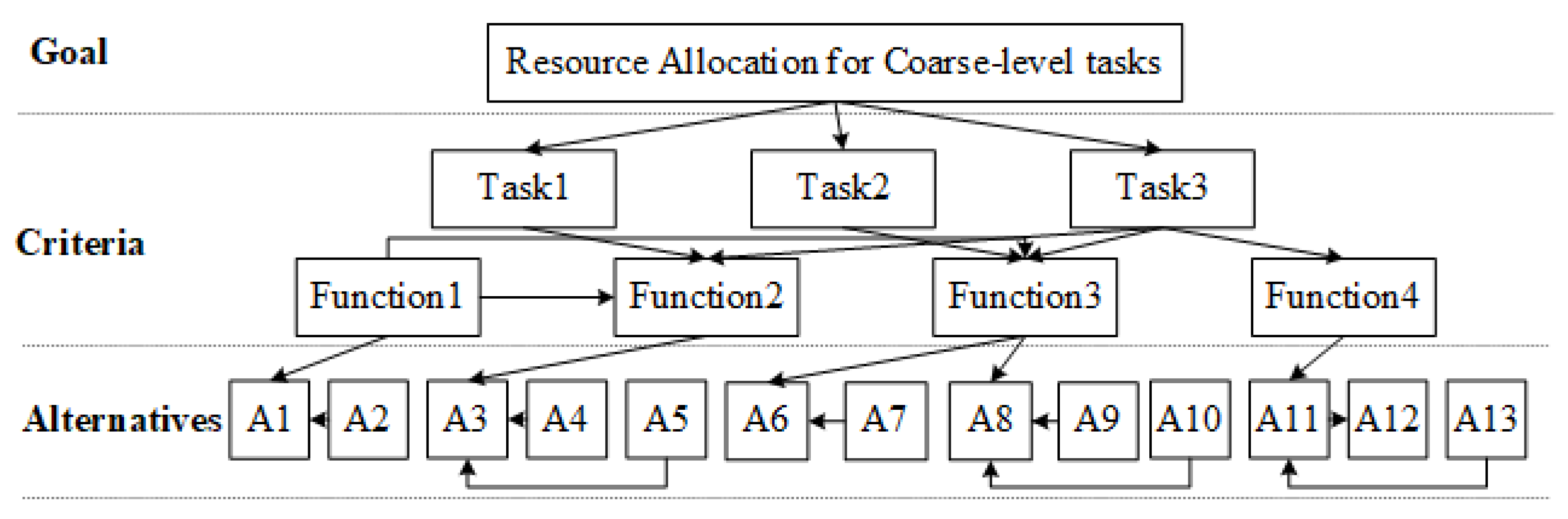
After the analysis, we complement the first phase of our method. The structure of MC is divided into Goal-layer, Criteria-layer, and Alternatives layer. Our target is to obtain the resource allocation strategy of ST for $MC$. Moreover, there are two sublayers in Criteria-layer. The whole structure is conducted as Figure 2 indicated. As the figure depicted, the inter-layers and intro-layers are interdependent. For example, Task 1 calls Function 2, and Function 2 needs A3, who calls A4 and A5 to work.

Figure 2. The Association Hierarchy Structure of Software MC (Note: “A → B” represents that B calls A to implement the task).

4.3.2. The Second Phase

After obtaining the framwork of $MC$, we carry out the second phase to predict the defect situation for Alternatives-layer. In the paper, we use the same 10 historical defect datasets from the other projects, as in paper [38]. The basic information about these data is listed in Table 5. For the target project $MC$, we use LDRA TESTBED, as mentioned in Section 4.2, to gain the metrics. Moreover, the linear regression model (LRM), which is applied in paper [38], is also used as the basic learner for predicting the result.

Table 5. The Basic Information about Historical Cross-project Defect Data.

Name	#Examples	#Metrics	Defect %	Source	Language	Description
ar1	147	29	6.12	Softlab	C	Embedded controller
ar4	117	29	17.01	Softlab	C	Embedded controller
cm1	352	21	11.93	NASA	C++	Spacecraft instrument
kc1	2096	21	15.51	NASA	C++	Storage management for ground data
kc3	194	39	18.56	NASA	Java	Storage managementfor ground data
mc2	125	21	35.20	NASA	C++	Video guidance system
mw1	253	37	11.49	NASA	C++	A zero gravity experiment
pc1	705	21	8.65	NASA	C++	Flight software
pc3	1125	21	12.44	NASA	C++	Flight software
pc4	1399	21	12.72	NASA	C++	Flight software

Finally, we obtain the predict result of Alternatives-layer, which is listed in Table 6. Therefore, the probability vector of the layer is as Formula (9).

$$P_{alter}={\left[0.0450.0270.0400.0270.0530.0220.0180.0200.0120.0120.1620.0640.057\right]}^T$$

(9)

Table 6. The Defect Probability of Alternatives-layer by Linear Regression Model (LRM) for $MC$.

ID	A1	A2	A3	A4	A5	A6	A7
Probability	0.045	0.027	0.040	0.027	0.053	0.022	0.018
ID	A8	A9	A10	A11	A12	A13
Probability	0.020	0.012	0.012	0.162	0.064	0.057

4.3.3. The Third Phase

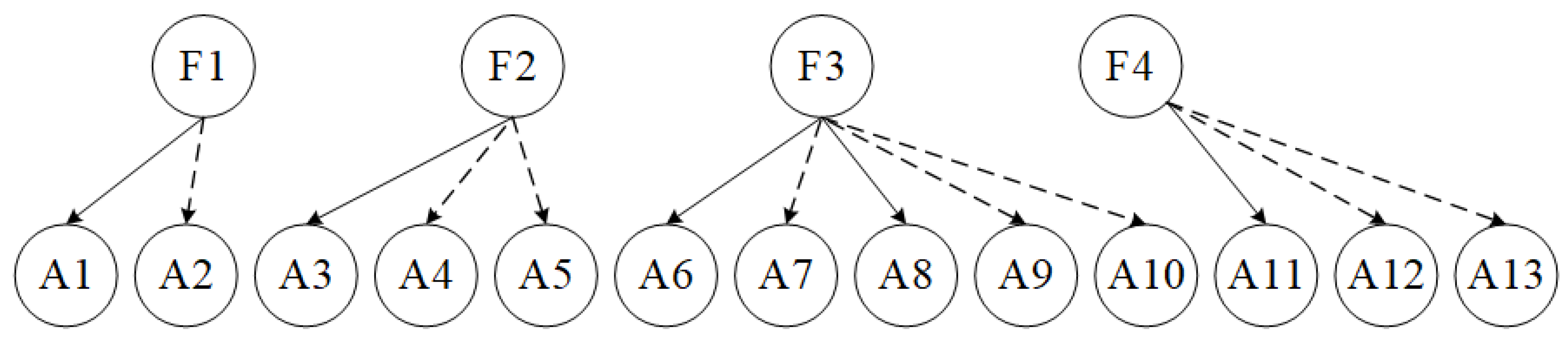
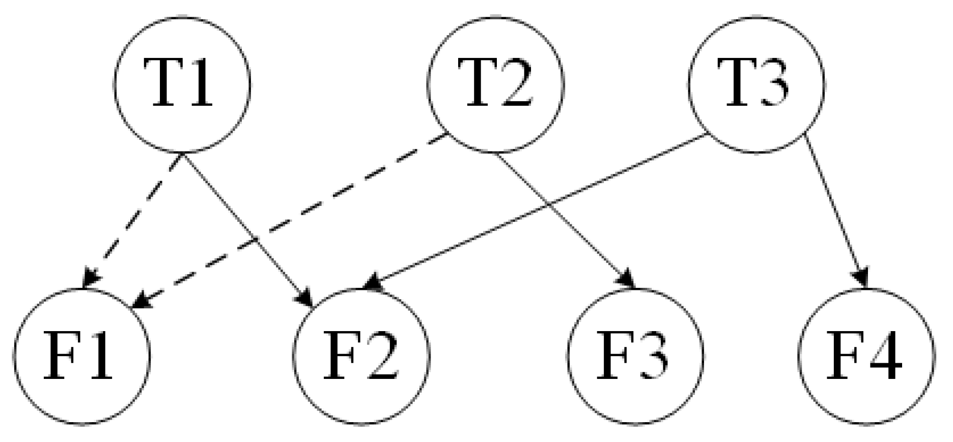
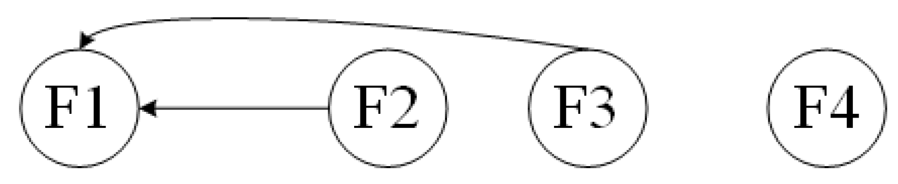
The graphs of Criteria-sublayer 1 (i.e., Function-layer) and Alternatives-layer from the structure of Figure 2 are shown as Figure 3 and Figure 4. The graphs of Criteria-sublayer (i.e., Task-layer) and Function-layer from the structure of Figure 2 are illustrated as Figure 5 and Figure 6.

Figure 3. The Vertical Graph of Function- and Alternatives-layer from The Association Hierarchy Structure of $MC$ (Note: the arrow from A to B represents that A calls B directly; the dash arrow from A to B means A calls B undirectly).

Figure 4. The Horinzonal Graph of Function-layer from The Association Hierarchy Structure of Software $MC$ (Note: the arrow from A to B represents that A calls B directly; the dash arrow from A to B means A calls B undirectly).

Figure 5. The Vertical Graph of Task- and Function-layer from The Association Hierarchy Structure of $MC$ (Note: the arrow from A to B represents that A calls B directly).

Figure 6. The Vertical Graph of Function-layer and from The Association Hierarchy Structure of $MC$.

As Figure 3 illustrated, the vertical PIM $H_{fa}$ between Function-layer and Alternatives-layer and the horizonal PIM of Function-layer are obtained. They are denoted as Formula (10) and Formula (11), respectively.

$$H_{fa}=\left[\begin{array}{ccccccccccccc}1& 1& 0& 0& 0& 0& 0& 0& 0& 0& 0& 0& 0\\ 0& 0& 1& 1& 1& 0& 0& 0& 0& 0& 0& 0& 0\\ 0& 0& 0& 0& 0& 1& 1& 1& 1& 1& 0& 0& 0\\ 0& 0& 0& 0& 0& 0& 0& 0& 0& 0& 1& 1& 1\end{array}\right]$$

(10)

$$H_{ff}=\left[\begin{array}{cccc}1& 0& 0& 0\\ 1& 1& 0& 0\\ 1& 0& 1& 0\\ 0& 0& 0& 1\end{array}\right]$$

(11)

As Figure 5 shows, the vertical PIM $H_{tf}$ between Task- and Function-layer is obtained as Formula (12). Because the elements of Task-layer are independent, the PIM $H_{tt}$ is obtained as Formula (13).

$$H_{tf}=\left[\begin{array}{cccc}1& 1& 0& 0\\ 1& 0& 1& 0\\ 0& 1& 0& 1\end{array}\right]$$

(12)

$$H_{tt}=\left[\begin{array}{ccc}1& 0& 0\\ 0& 1& 0\\ 0& 0& 1\end{array}\right]$$

(13)

4.3.4. The Four Phase

In the last phase, we derive the defect probability of each element in Criteria-layer. For the Function-layer, their defect probability vector $P_{fun}$ are as Formula (14). Besides, the probability vector $P_{task}$ of the Task-layer is displayed in Formula (15).

$$P_{fun}=H_{ff}\times H_{fa}\times P_{alter}={\left[\begin{array}{cccc}0.072& 0.192& 0.156& 0.283\end{array}\right]}^T$$

(14)

$$P_{task}=H_{tt}\times H_{tf}\times P_{fun}={\left[\begin{array}{ccc}0.264& 0.228& 0.475\end{array}\right]}^T$$

(15)

We normalize the $P_{task}$ by Formula (8). Subsequently, we obtain the normalized defect probability values of the three tasks (i.e., 0.146, 0, 1).

5. Results Analysis and Discussion

RQ1: How is SDP used for coarse-level tasks of software testing?

For RQ1, the result of $P_{task}$ indicates that Task 2 is the least defective and Task 3 is the most defective. If a test leader or manager does not know the prediction result in advance, he or she will divide the resource evenly and make the testers test each task randomly. However, when the defectiveness of each task is predicted, the test leader or manager needs to arrange more resource for Task 3, less resource for Task 2. Besides, for test resource, it includes number of test cases, testers, test environment (such as, test tool, test devices, support staff), time, budget, etc.

For instance, the test manager totally has four test environments and four testers of equivalent professional level to execute ST for the three tasks. According to the coarse-level predict result, the manager can arrange two testers to check Task 3, one tester to check Task 2, and the left one to check Task 1. Besides, For Task 3 and Task 2, testers can use two days. However, for Task1, it is enough for the tester to use one day.

RQ2: Can DPAHM complement different defect prediction task types?

From the processes of DPAHM in Section 3 and the implementation steps of an example software $MC$ in Section 4.3, we can realize that the result of SDP for Alternatives-level is an input value for coarse-level prediction. Thus, the final result form of coarse-level totally depends on the input value form. That is, the prediction granularity of the SDP result is binary, numeric, or ranking labels according to the SDP model which relies on prediction learners. For example, if a machine learning technique for regression task is chosen as a basic learner, the result from SDP on Alternatives-level will be numeric and the result of coarse-level will be the number of defect in each element of the Criteria-layer.

Therefore, for RQ2, the answer is “YES”.

RQ3: How do different defect prediction learners affect DPAHM?

For RQ3, we can analyze from two different perspectives:

One perspective is to discuss the effect of the prediction tasks. Because of RQ2, we know DPAHM can finish different prediction tasks. Therefore, we analyze how the different prediction tasks affect DPAHM. For classification models of SDP, the result of coarse-level tasks is binary. Each task will be predicted as defective or non-defective. The project manager cannot obtain extra information for all tasks. Therefore, the resource allocation strategy is coarse, but better than evenly resource allocation. For regression models of SDP, the result is numeric or ranking. For ranking result, the project manager can manage the resource according to the order. For numeric result, the manager can not only arrange the resource according to the numeric values, but also design different test cases to find these bugs. Therefore, we advise practitioners to do numeric or ranking prediction tasks. Because the result will provide more detailed information for resource allocation than classification prediction tasks.

The other perspective is the different learners for the same prediction tasks. Different learners may indicate different prediction results [9,38]. For ranking prediction tasks as examples, Xiao et al. analyzed the effect of different learners (i.e., LRM, Random Forest, and gradient boost regression tree) on FIP [38], we use the same prediction approach as a basic SDP model. Therefore, we do not use the other learners for our experiment. Our final prediction result relies on the result of the Alternatives-layer. Therefore, the practitioners need to select a proper learner according to what result you want to get.

6. Threats to Validity

Potential threats to the validity of our research method are shown as follows.

Threats to internal validity: we use the SDP technique as the basic method for coarse-level tasks. The datasets we used in the experiment are cleaned, which means 18 common metrics are used and similar instances with software MC from cross-projects are selected. Besides, we have checked our experiments four times by all of the authors, there may still be some errors. Moreover, to the best of our knowledge, it is the first time to apply SDP for coarse-level tasks. Therefore, we did not execute control experiments. However, we explain the advantage of our proposed approach as compared with the uncertainty of evenly allocating resources.

Threats to external validity: we have verified the effectiveness of DPAHM via applying it to a specific software. Moreover, we only use LRM to make defect prediction for Alternatives-layer. Because our goal is to provide a method about allocating test resource for coarse-level tasks instead of finding the best model for the tasks. In order to generalize our proposed approach, we analyze the different types SDP methods (i.e., classification, ranking, numeric types) of DPAHM. In the future, more software for coarse-level tasks should be considered to reduce external validity.

Threats to construct validity: DPAHM relates to AHP and PIM. Therefore, the framework and relationships are important for the final result. We carefully check and draw the structure via the specifications and codes. In addition, our proposed DPAHM is based on SDP. According to previous SDP studies [14,38,63], different performance measures are used. In the paper, we just follow paper [38] and also use PoD to assess the performance of SDP in the Alternatives-layer.

7. Conclusions and Future Work

To alleviate the difficult resource allocation situation without execution information for coarse-level tasks, an approach, called DPAHM, is proposed in this paper. The method regards the resource allocation problem for ST as a multiple decision-making problem and combine AHP with a variation of incidence matrix to predict the defect situation of coarse-level tasks based on SDP techniques. Thus, the corresponding resource allocation strategy is born.

The approach is divided into four phases: association hierarchy framework conduction phase, software defect prediction model establishment phase, positive incidence matrix from vertical and horizonal direction production phase, and resource allocation strategy output phase. We apply the proposed method to a true software $MC$ and the result indicates our method can provide ideas about resource allocation strategies for coarse-level testing tasks, such as system-level testing.

In the study, we aim at resource allocation for coarse-level tasks of ST. Accordingly, we only depend on SDP to predict defect situation for coarse-level tasks. DPAHM provides guidance for allocating resource. In the future, we will collect more resource allocation information (such as the number of test cases executed by each person every day, proportion of system testing time, budget for each person) to optimize the allocation strategy. Moreover, we assume that the call relationship between fine- and coarse-level is known or obtained by analysis. However, for complex software, it is difficult to analyze the association or hierarchy structure. Therefore, it is another direction in the future to provide resource allocation strategies for the coarse-level tasks of complex software.