Dynamic Behavior of Steel and Composite Ferry Subjected to Transverse Eccentric Moving Load Using Finite Element Analysis

Abstract
1. Introduction
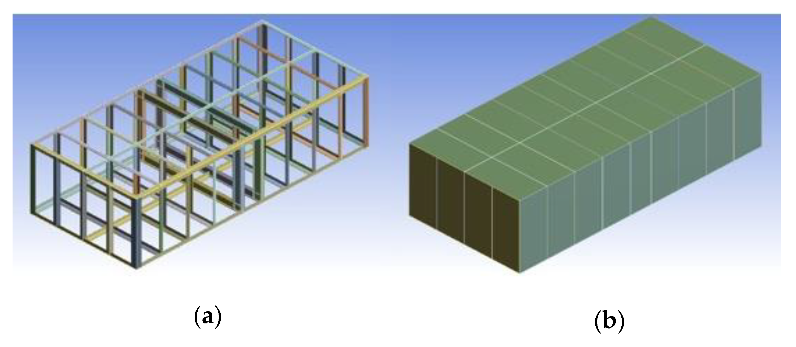
2. Finite Element Modeling of the Steel Ferry
3. Model Definition
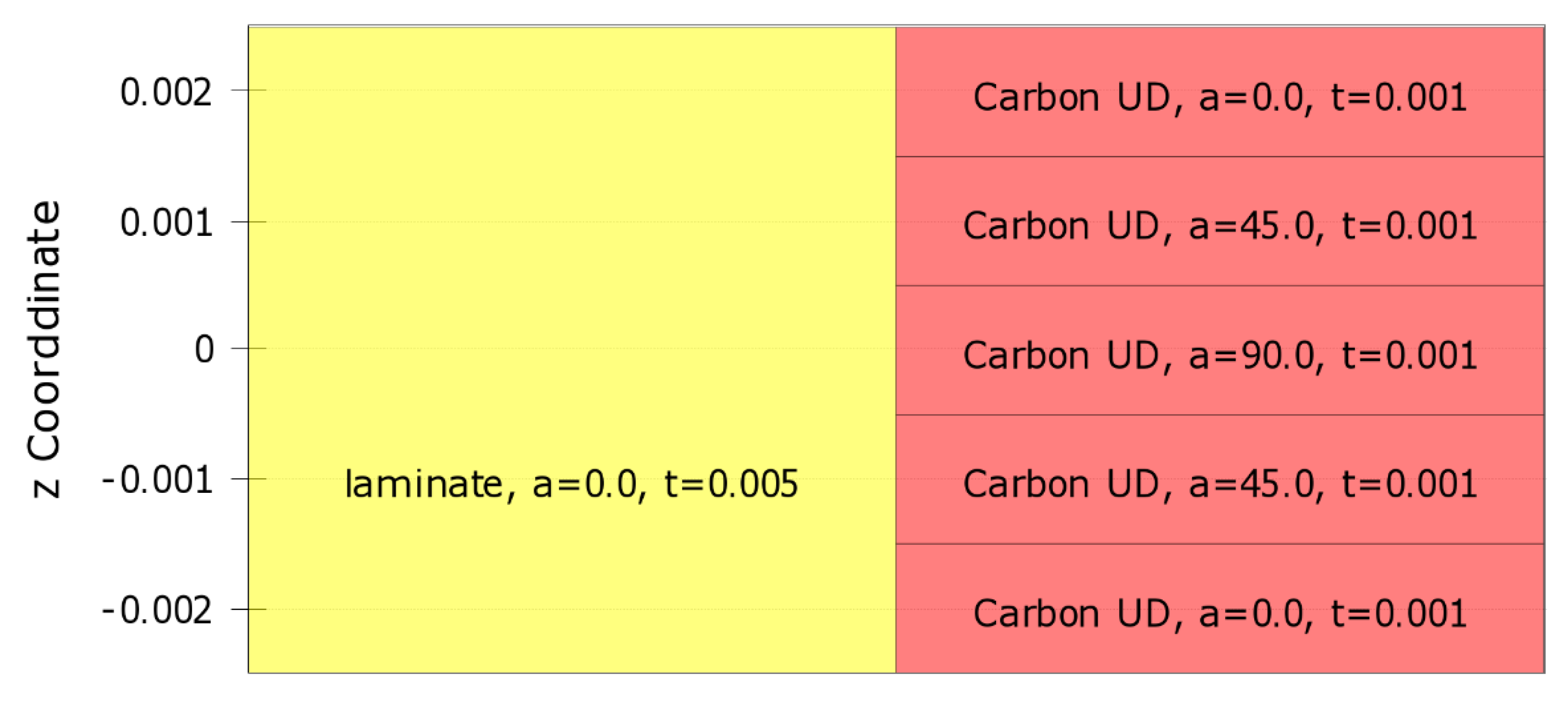
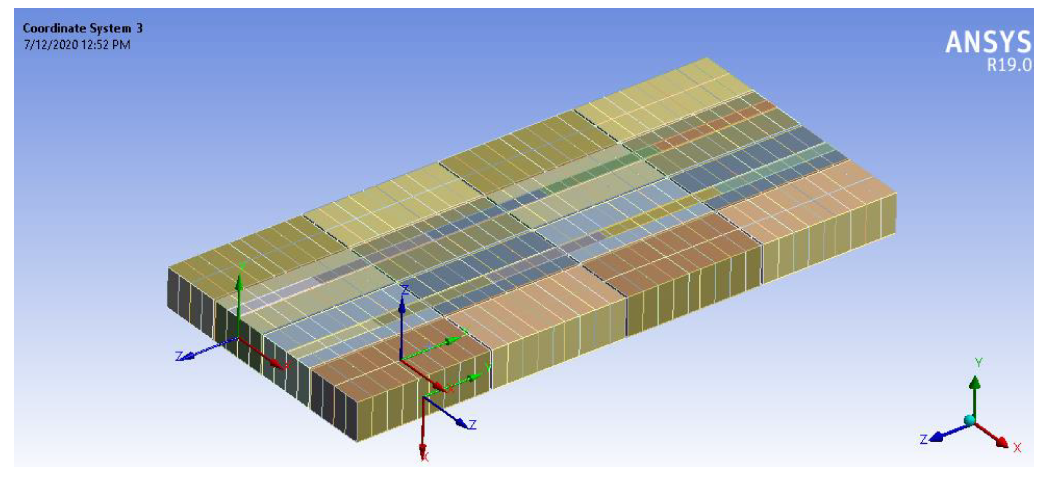
3.1. Geometry and Material
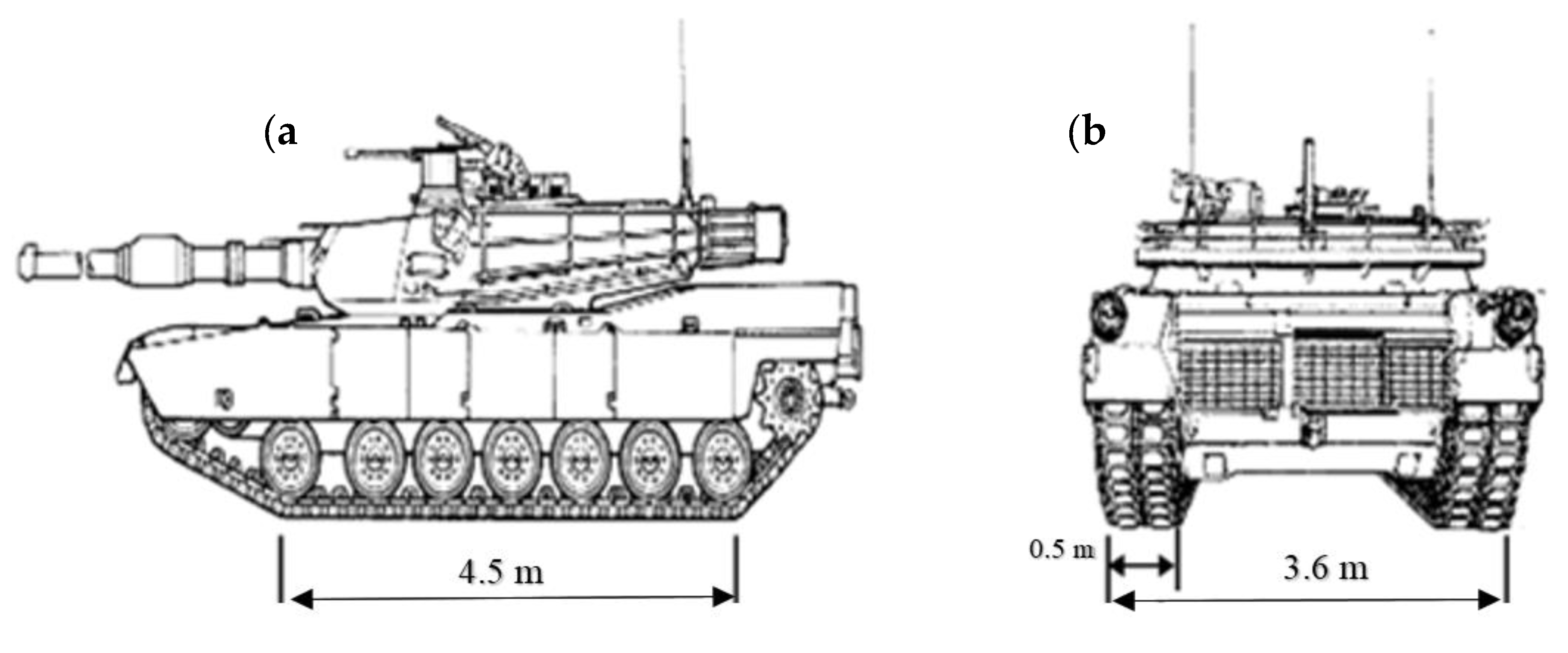
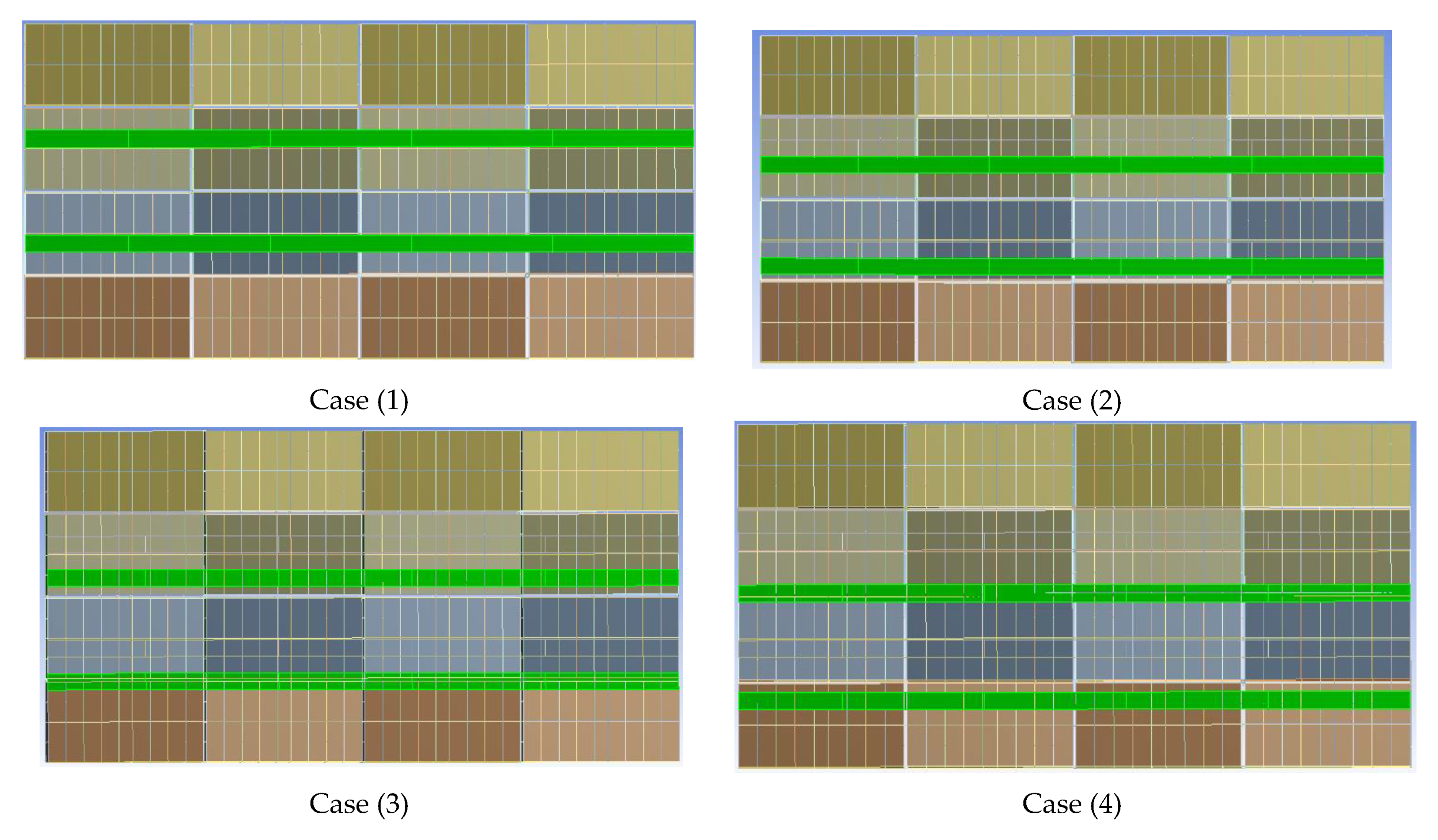
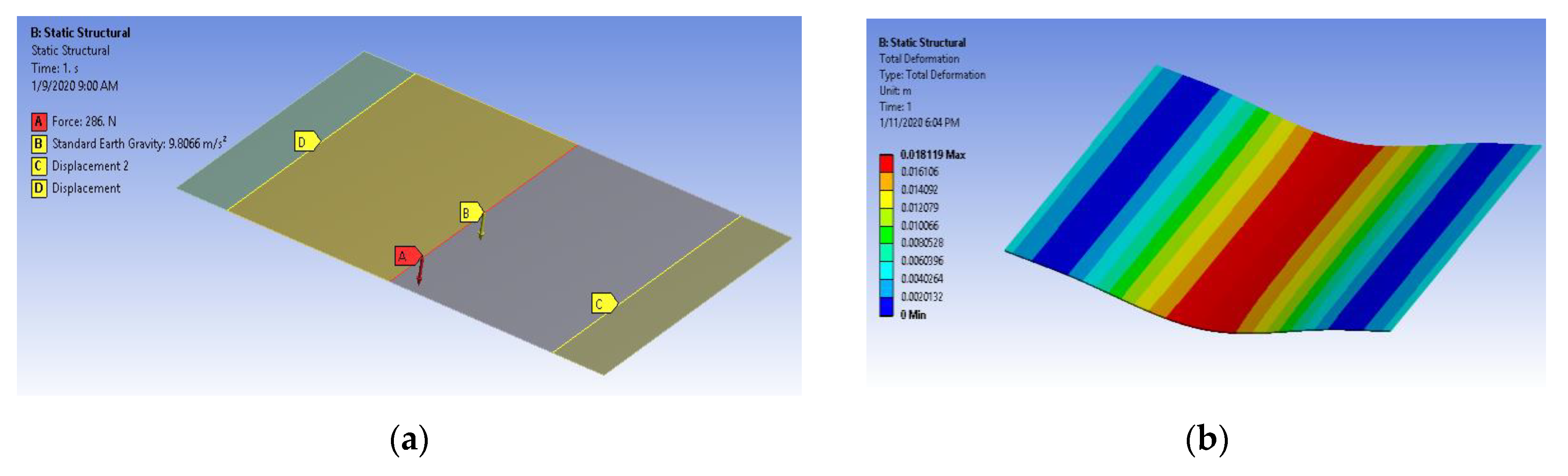
3.2. Loads
3.3. Boundary Conditions
3.4. Elastic Support Stiffness
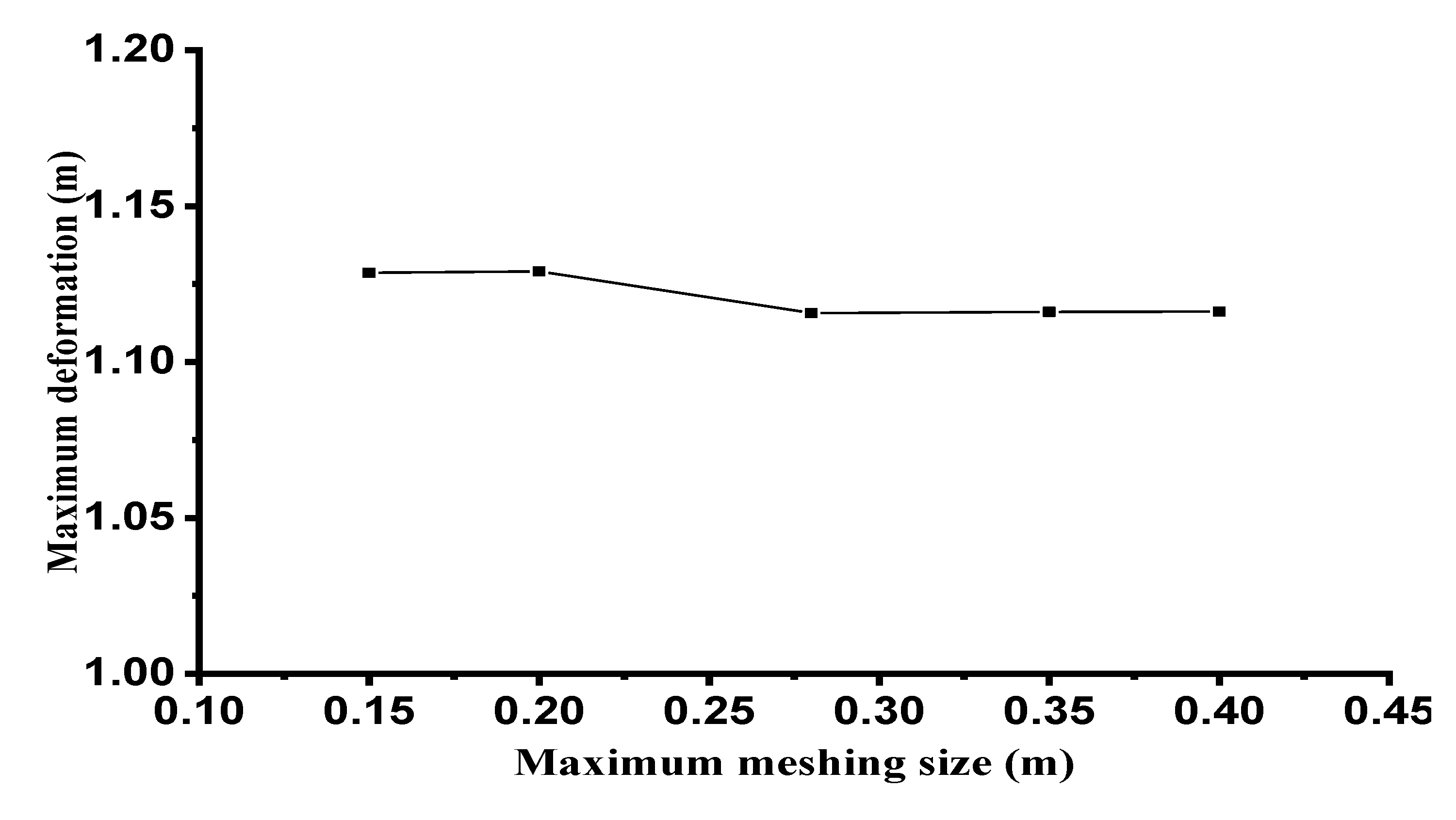
3.5. Convergence Study
4. Validation
5. Composite Ferry
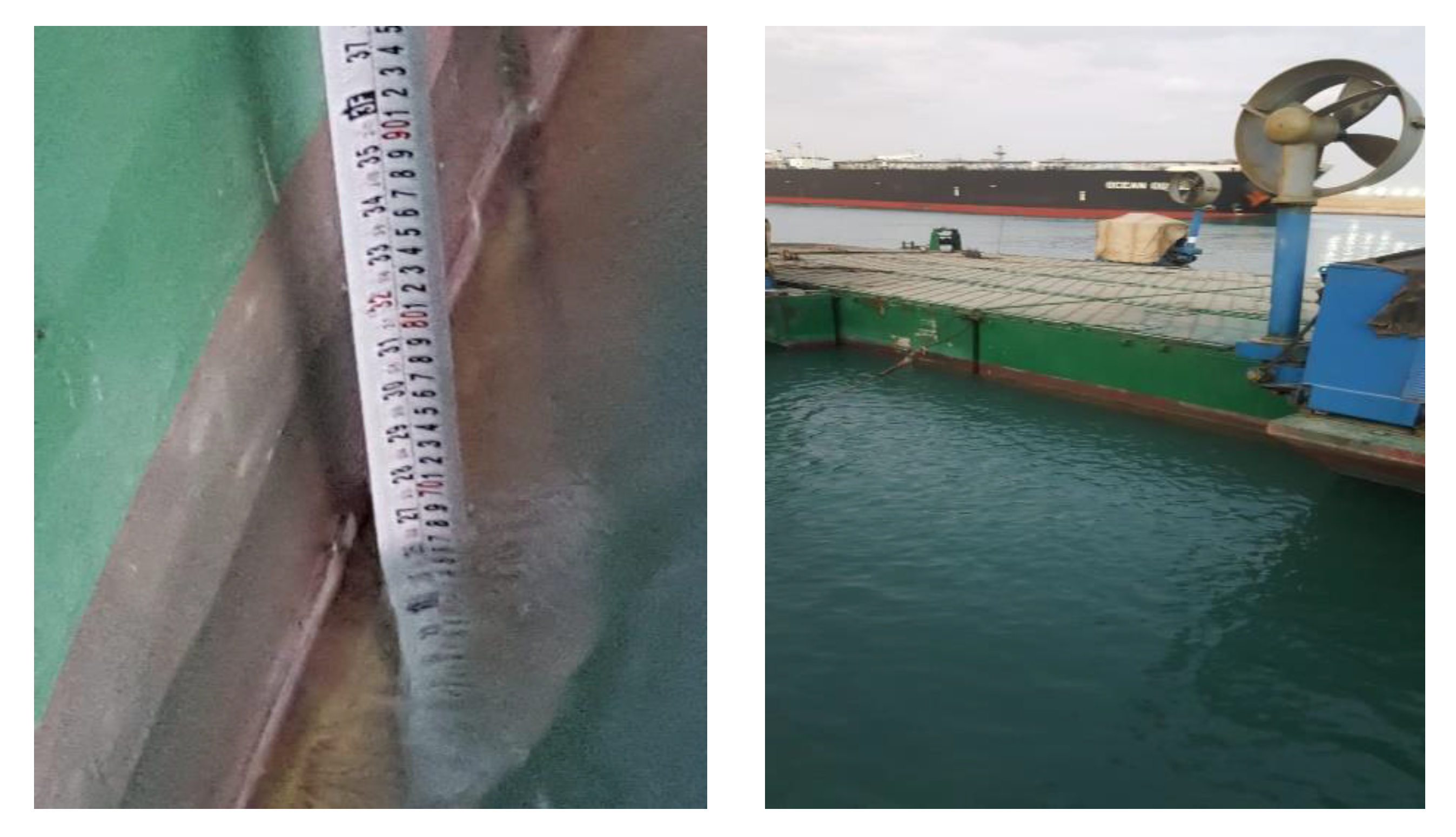
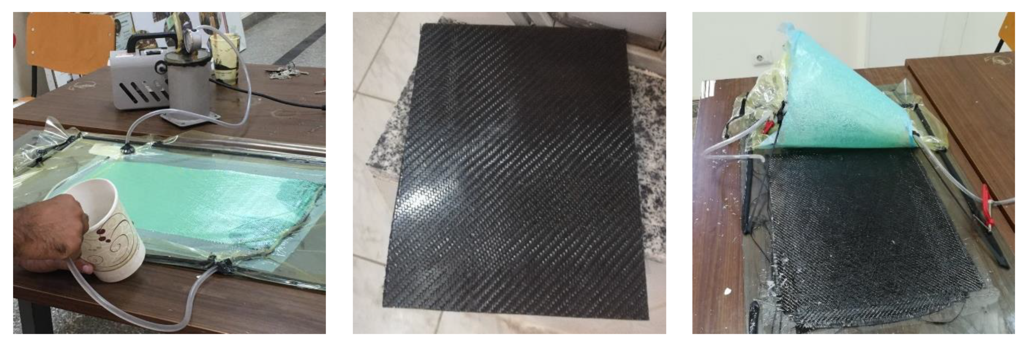
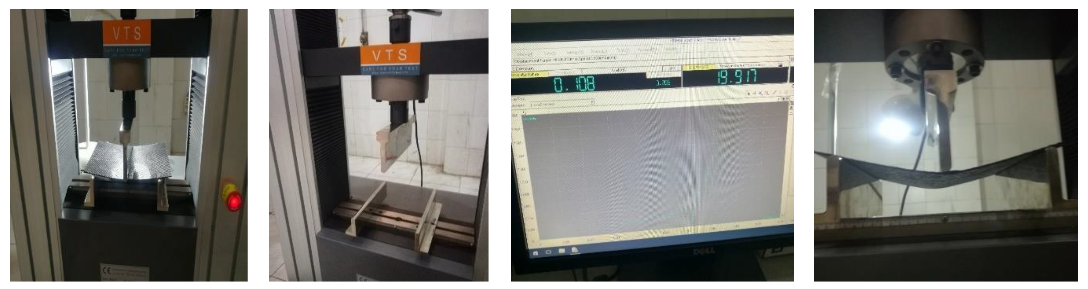
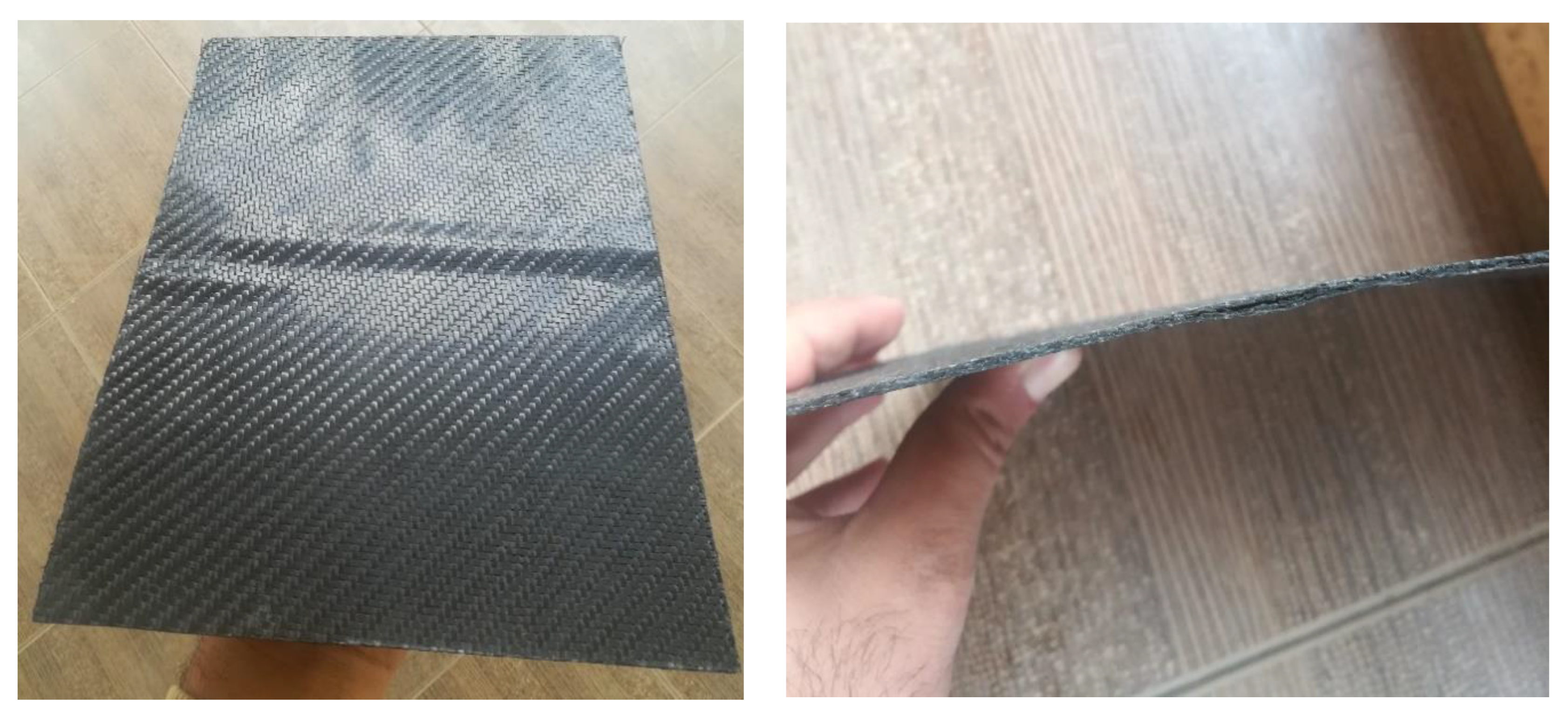
5.1. Practical Validation for CFRP
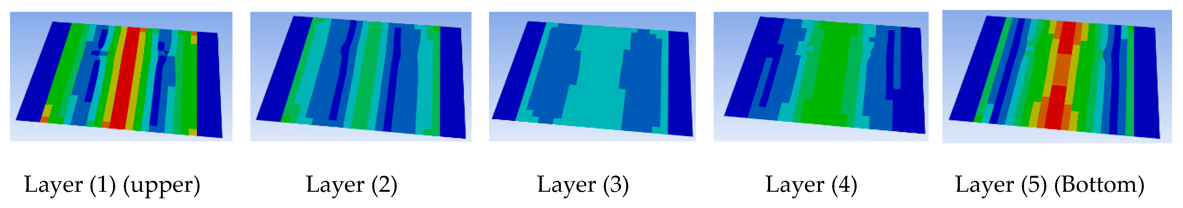
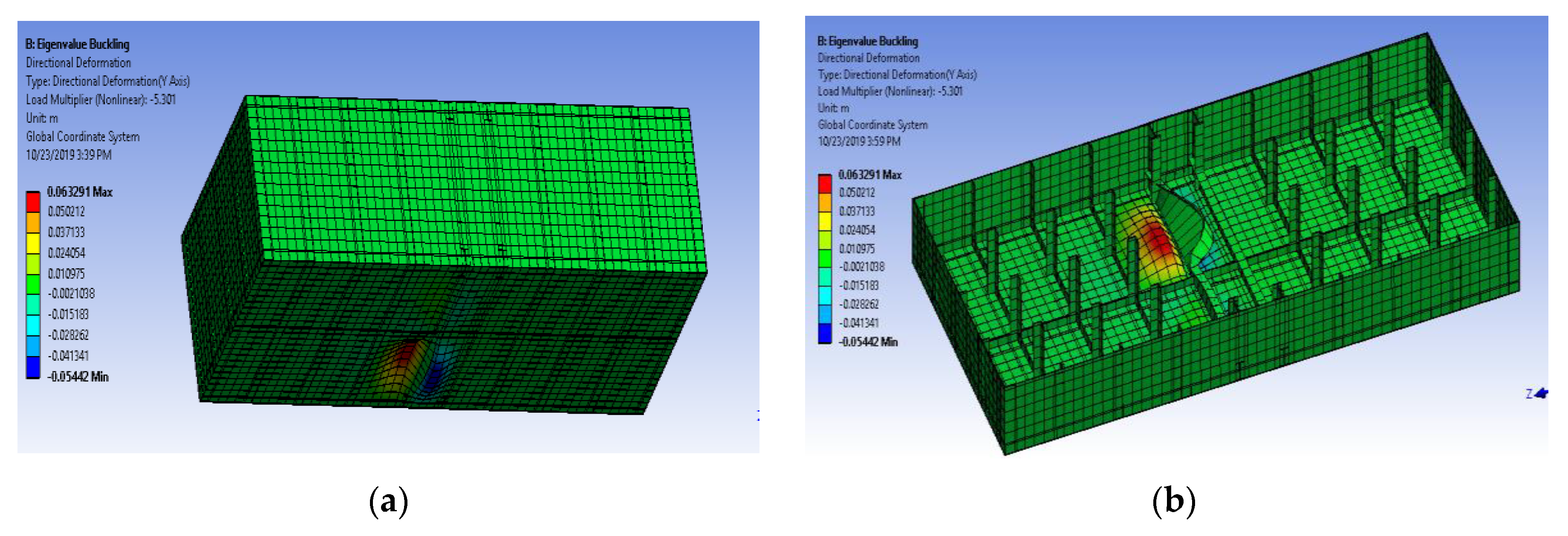
5.2. Nonlinear Buckling Analysis
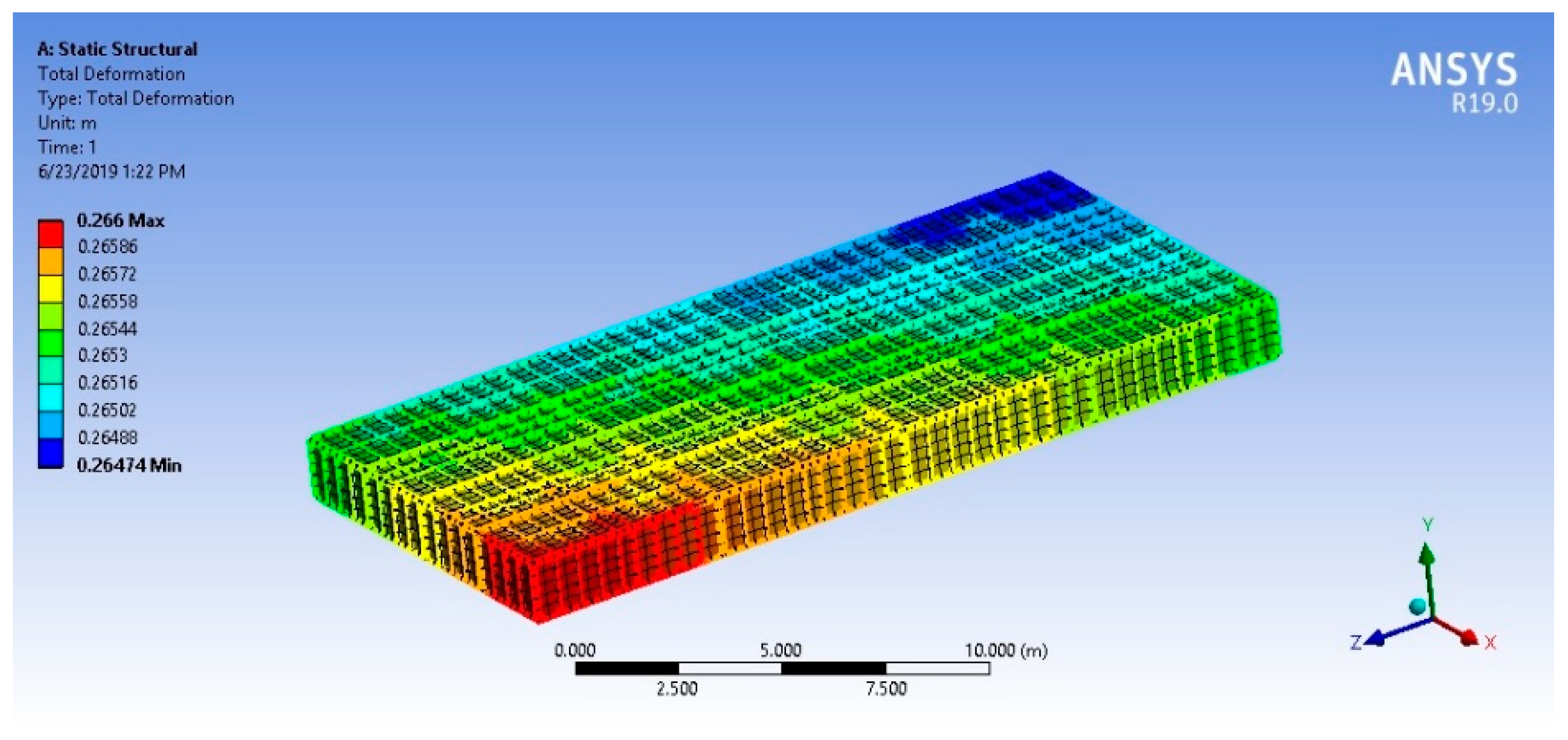
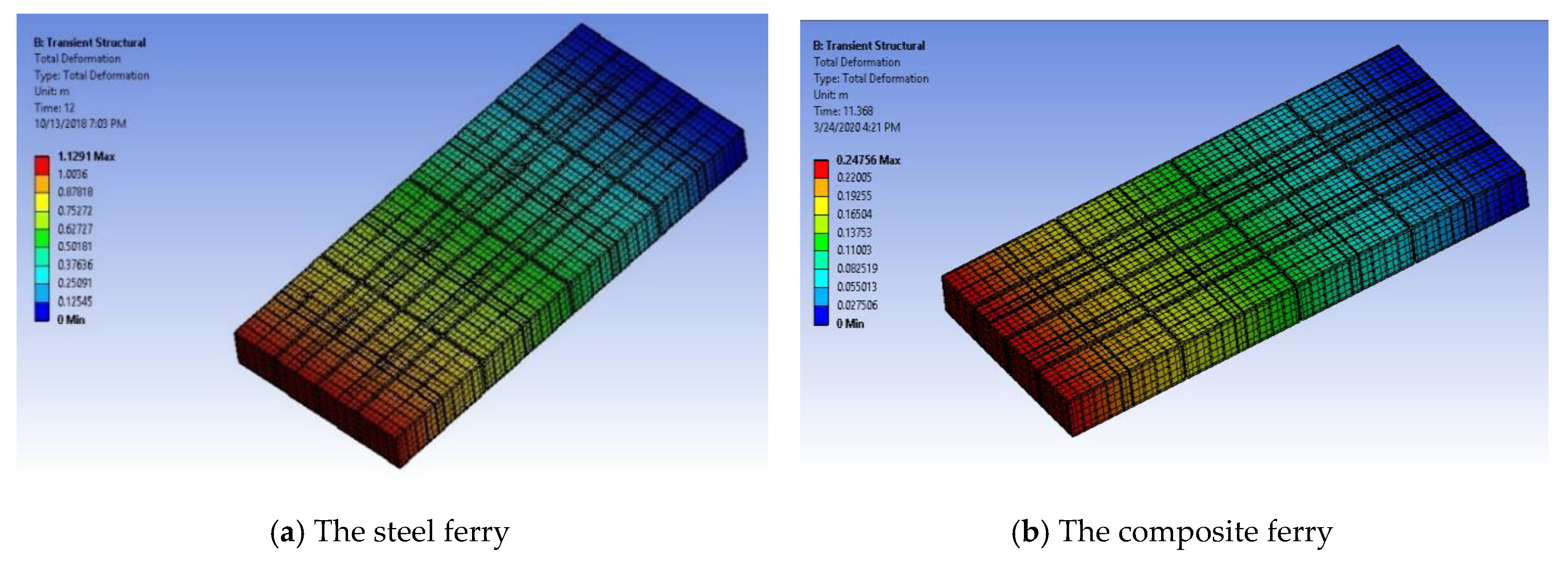
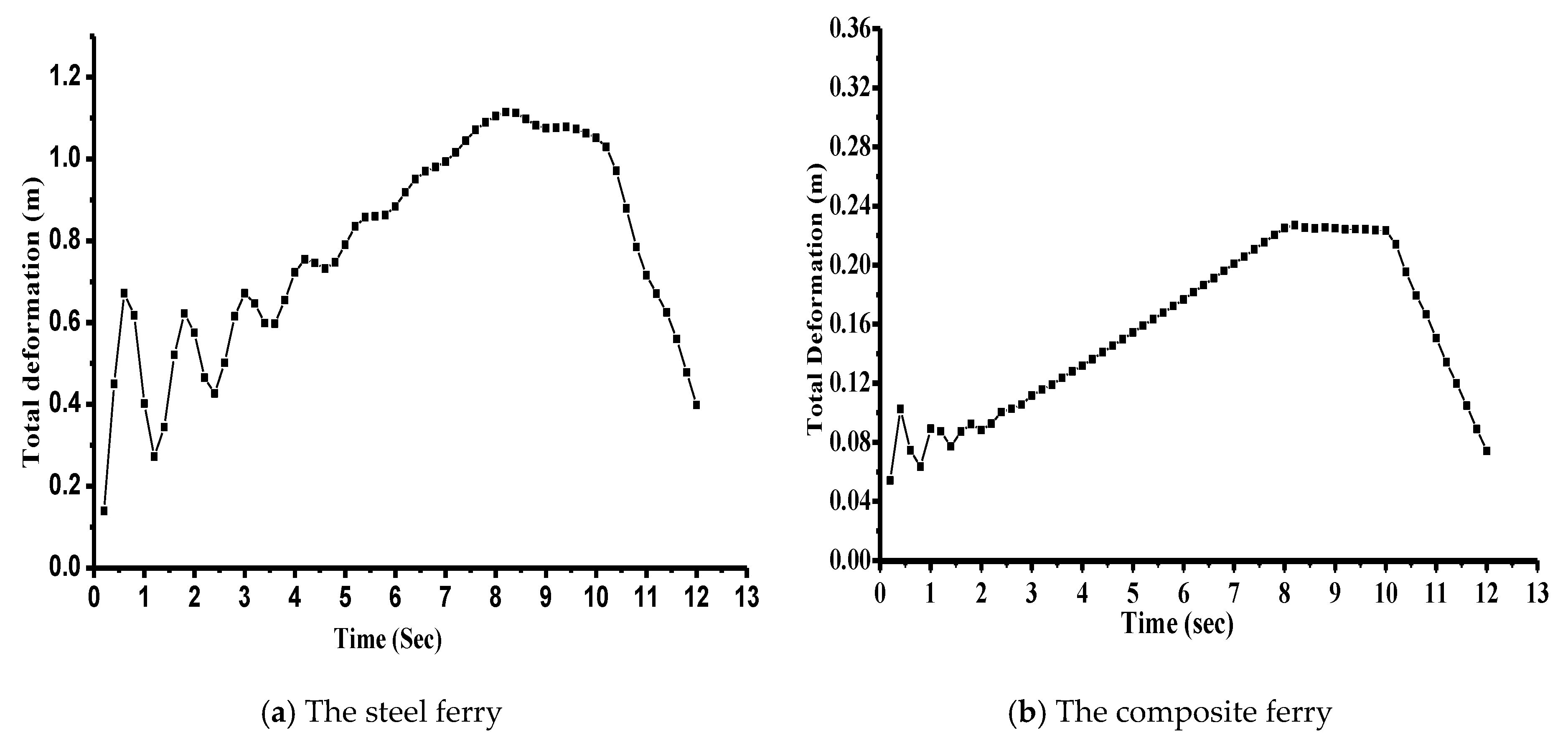
6. Results and Discussion
6.1. Case 1
6.2. Case 2
6.3. Case 3
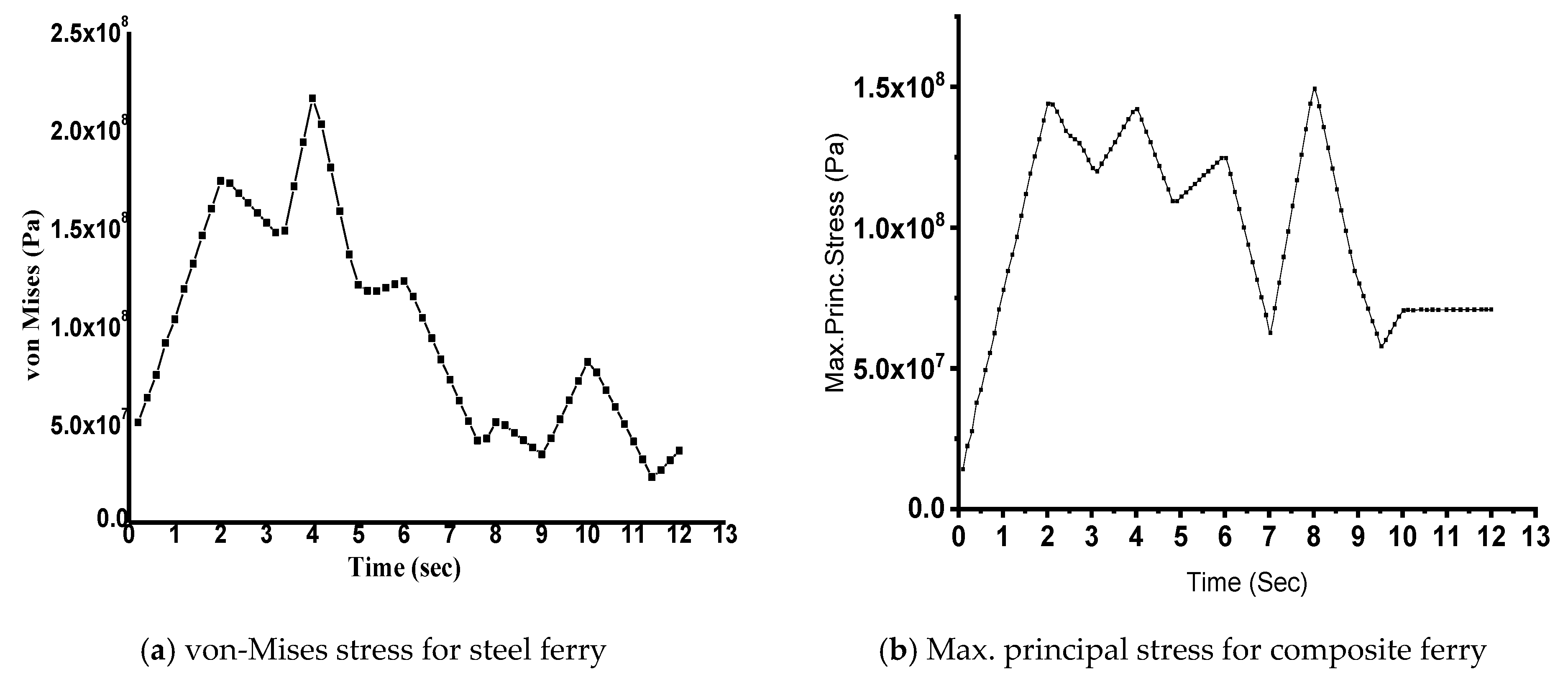
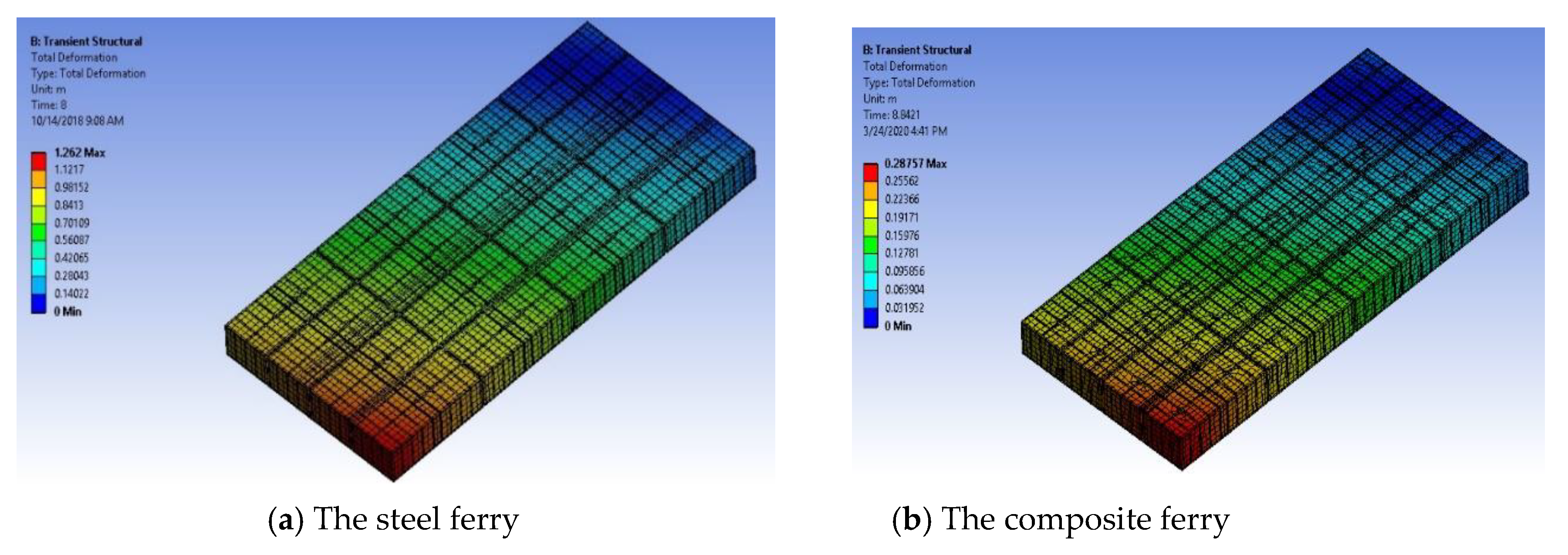
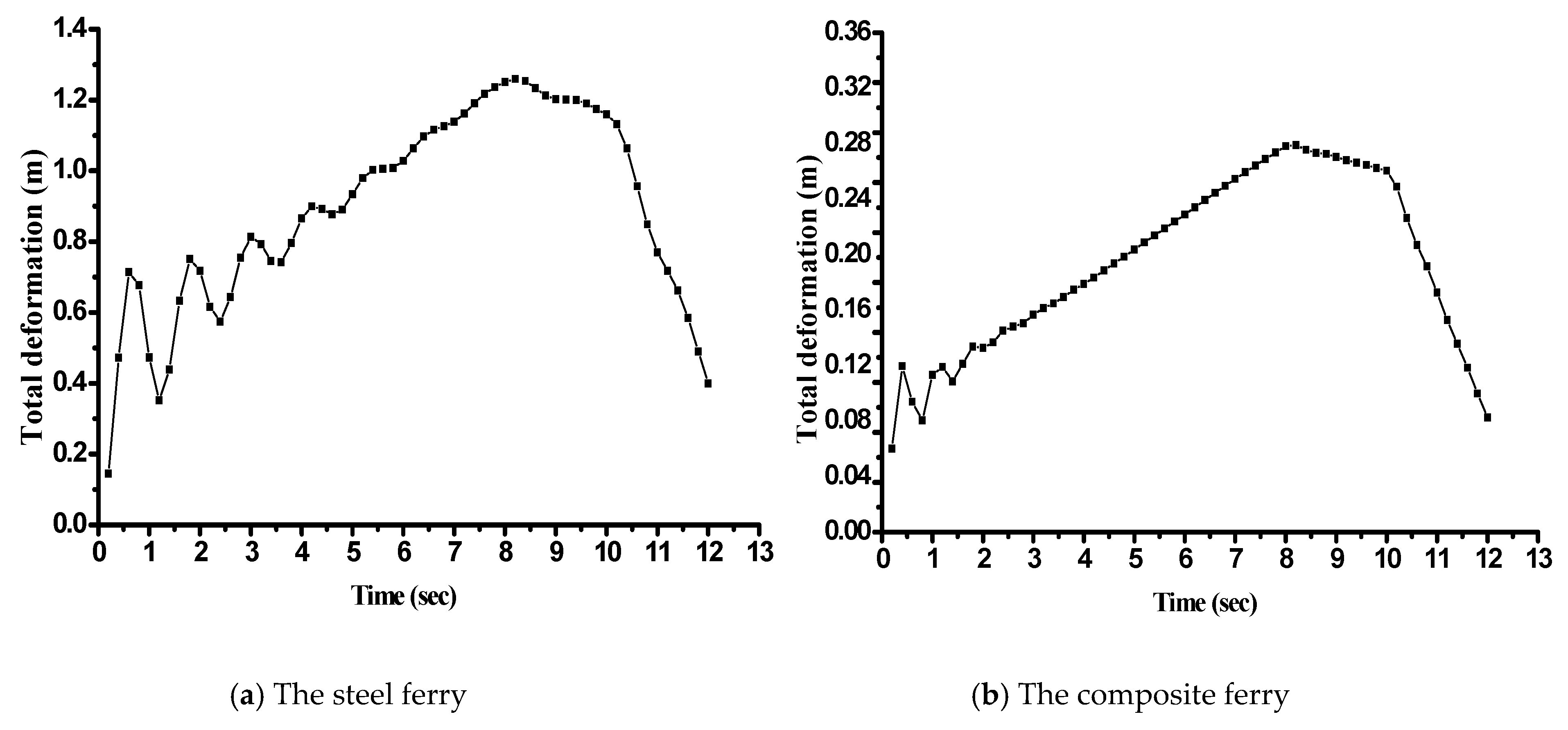
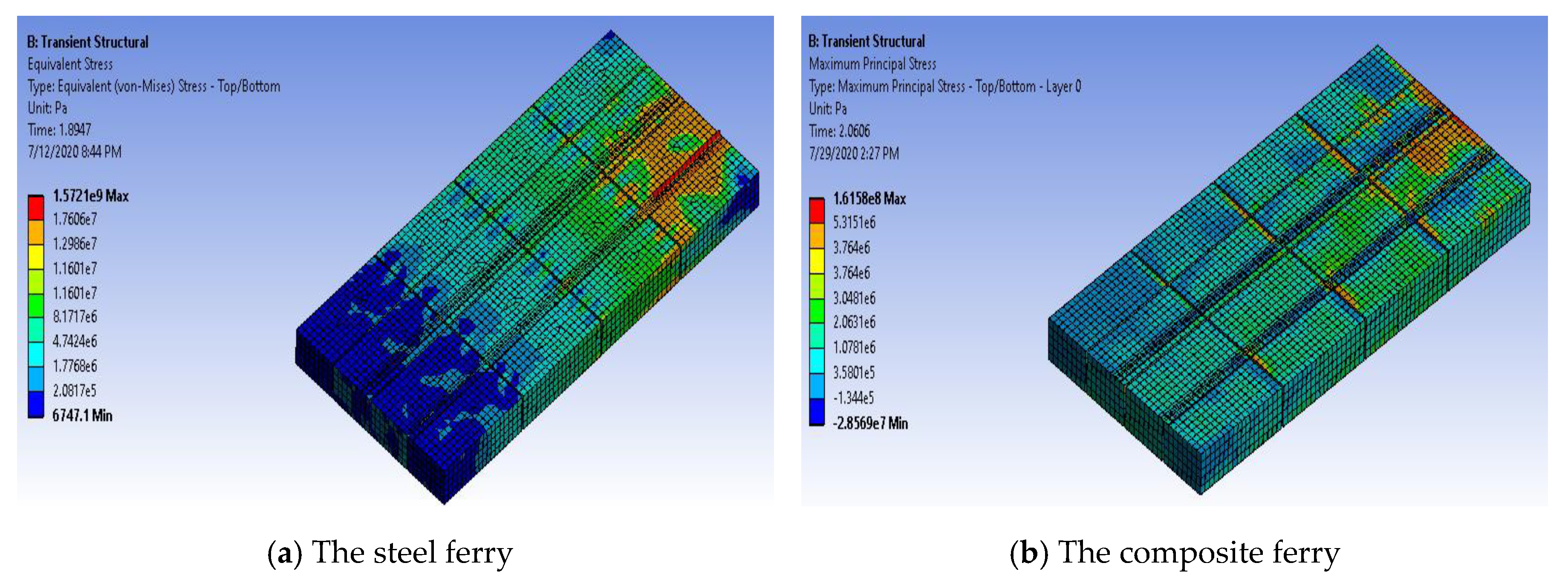
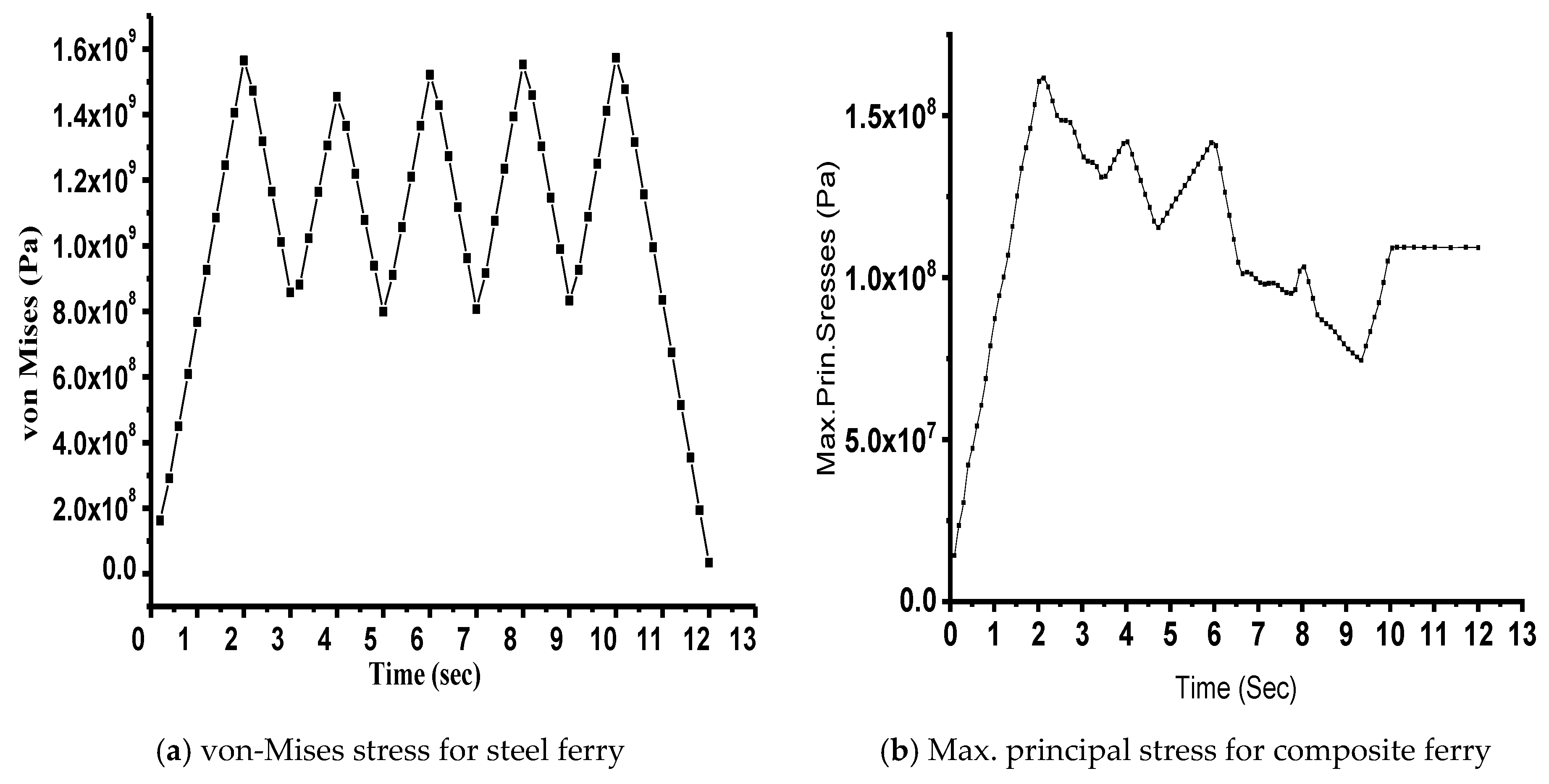
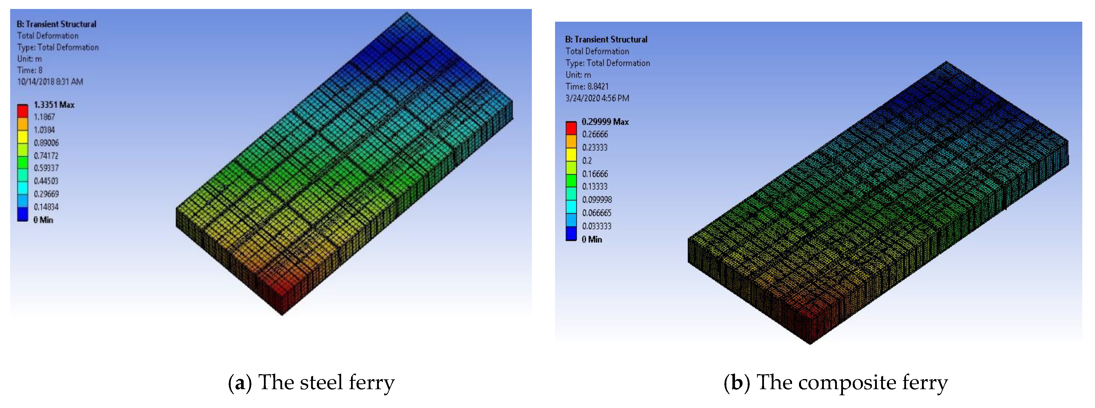
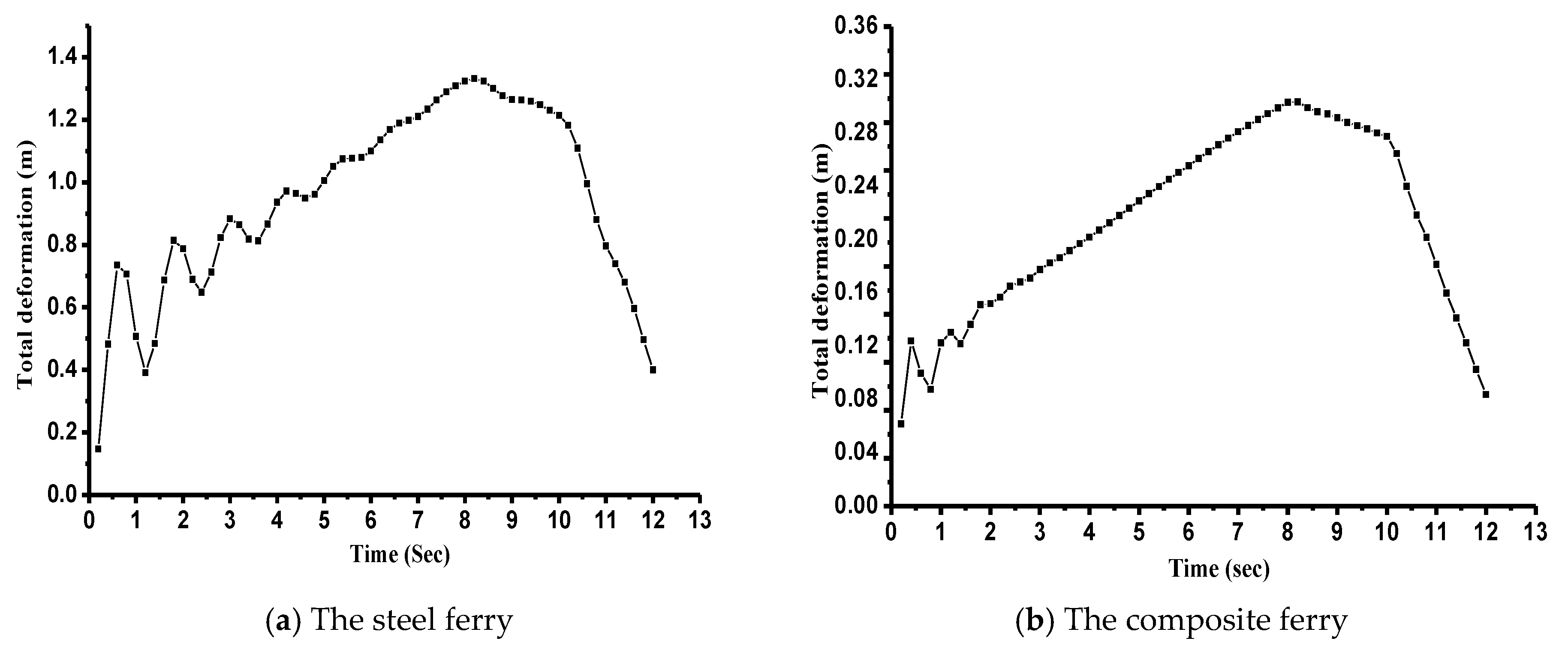
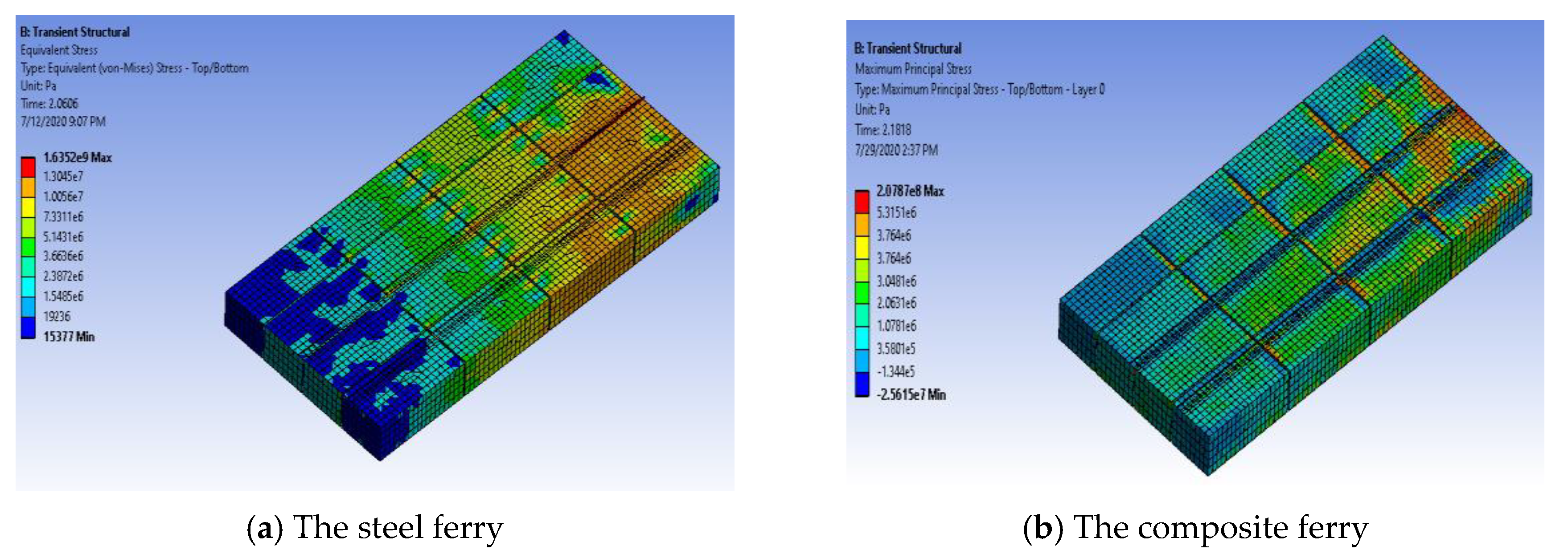
6.4. Case 4
7. Conclusions
Author Contributions
Funding
Acknowledgments
Conflicts of Interest
References
- Cheng, Z.; Gao, Z.; Moan, T. Wave load effect analysis of a floating bridge in a fjord considering inhomogeneous wave conditions. Eng. Struct. 2018, 163, 197–214. [Google Scholar] [CrossRef]
- Watanabe, E.; Utsunomiya, T. Analysis and design of floating bridges. Prog. Struct. Eng. Mater. 2003, 5, 127–144. [Google Scholar] [CrossRef]
- Sun, J.; Jiang, P.; Sun, Y.; Song, C.; Wang, D. An experimental investigation on the nonlinear hydroelastic response of a pontoon-type floating bridge under regular wave action. Ships Offshore Struct. 2017, 13, 233–243. [Google Scholar] [CrossRef]
- Shahrabi, M.; Bargi, K. Numerical simulation of multi-body floating piers to investigate pontoon stability. Front. Struct. Civ. Eng. 2013, 7, 325–331. [Google Scholar]
- Zhang, J.; Miao, G.-P.; Liu, J.-X.; Sun, W.-J. Analytical Models of Floating Bridges Subjected by Moving Loads for Different Water Depths. J. Hydrodyn. 2008, 20, 537–546. [Google Scholar] [CrossRef]
- Hirono, Y. Positional displacement measurement of floating units based on aerial images for pontoon bridges. In International Conference on Advanced Engineering Theory and Applications; Springer: Berlin/Heidelberg, Germany, 2016. [Google Scholar]
- Wu, J.-S.; Shih, P.-Y. Moving-load-induced vibrations of a moored floating bridge. Comput. Struct. 1998, 66, 435–461. [Google Scholar] [CrossRef]
- Ibrahim, M.M.; Hassan, M.A.; Ghanim, A.D. Effect of Floating Bridges on Velocity Distribution. J. Eng. Res. Rep. 2019, 1–16. [Google Scholar] [CrossRef]
- Fu, S.; Cui, W. Dynamic responses of a ribbon floating bridge under moving loads. Mar. Struct. 2012, 29, 246–256. [Google Scholar] [CrossRef]
- Khalifa, Y.A. Study the Structural System Effect on the Stability of Floating Metallic Bridges. Ph.D. Thesis, Military Technical College, Cairo, Egypt, 2008. [Google Scholar]
- Raftoyiannis, I.G.; Avraam, T.P.; Michaltsos, G.T. Analytical models of floating bridges under moving loads. Eng. Struct. 2014, 68, 144–154. [Google Scholar] [CrossRef]
- Wang, H.-H.; Jin, X.-L. Dynamic analysis of maritime gasbag-type floating bridge subjected to moving loads. Int. J. Nav. Arch. Ocean Eng. 2016, 8, 137–152. [Google Scholar] [CrossRef]
- Jun, Z.; Liu, J.; Ni, X.L.; Li, W.; Mu, R.; Zhang, J. Dynamic Model of a Discrete-Pontoon Floating Bridge Subjected by Moving Loads. Appl. Mech. Mater. 2010, 29, 732–737. [Google Scholar] [CrossRef]
- Nguyen, X.V. A Moving Element Method for Hydroelastic Response of a Floating Thin Plate Due to a Moving Load. In ACMSM25; Springer: Berlin/Heidelberg, Germany, 2020; pp. 189–198. [Google Scholar]
- Dai, J.; Leira, B.J.; Moan, T.; Kvittem, M.I. Inhomogeneous wave load effects on a long, straight and side-anchored floating pontoon bridge. Mar. Struct. 2020, 72, 102763. [Google Scholar] [CrossRef]
- Kvåle, K.A.; Sigbjörnsson, R.; Øiseth, O. Modelling the stochastic dynamic behaviour of a pontoon bridge: A case study. Comput. Struct. 2016, 165, 123–135. [Google Scholar] [CrossRef]
- Taetragool, U.; Shah, P.; Halls, V.; Zheng, J.; Batra, R.C. Stacking sequence optimization for maximizing the first failure initiation load followed by progressive failure analysis until the ultimate load. Compos. Struct. 2017, 180, 1007–1021. [Google Scholar] [CrossRef]
- Tsai, S.W.; Wu, E.M. A General Theory of Strength for Anisotropic Materials. J. Compos. Mater. 1971, 5, 58–80. [Google Scholar] [CrossRef]
- Helal, M.; Huang, H.; Wang, D.; Fathallah, E. Numerical Analysis of Sandwich Composite Deep Submarine Pressure Hull Considering Failure Criteria. J. Mar. Sci. Eng. 2019, 7, 377. [Google Scholar] [CrossRef]
- Kim, T.W.; Lee, D.H.; Trong, V.; Son, C.H.; Yoon, J.I.; Choi, K.H.; Kim, Y.B. A Study on Motion Control of Multiple Floating Units. In Proceedings of the 4th World Congress on Mechanical, Chemical, and Material Engineering, Madrid, Spain, 16–18 August 2018. [Google Scholar]
- Fathallah, E.; Qi, H.; Tong, L.; Helal, M. Design optimization of lay-up and composite material system to achieve minimum buoyancy factor for composite elliptical submersible pressure hull. Compos. Struct. 2015, 121, 16–26. [Google Scholar] [CrossRef]
- Fathallah, E. Optimal Design Analysis of Composite Submersible Pressure Hull. Appl. Mech. Mater. 2014, 578, 89–96. [Google Scholar]
- Helal, M.; Fathallah, E. Multi-Objective optimization of an intersecting elliptical pressure hull as a means of buckling pressure maximizing and weight minimization. Mater. Test. 2019, 61, 1179–1191. [Google Scholar] [CrossRef]
- Kim, S.-H.; Yoon, S.J.; Choi, W. Design and Construction of 1 MW Class Floating PV Generation Structural System Using FRP Members. Energies 2017, 10, 1142. [Google Scholar] [CrossRef]
- Imran, M.; Shi, D.; Tong, L.; Waqas, H.M.; Muhammad, R.; Uddin, M.; Khan, A. Design Optimization and Non-Linear Buckling Analysis of Spherical Composite Submersible Pressure Hull. Materials 2020, 13, 2439. [Google Scholar] [CrossRef]
- Omidali, M.; Khedmati, M.R. Reliability-Based design of stiffened plates in ship structures subject to wheel patch loading. Thin Walled Struct. 2018, 127, 416–424. [Google Scholar] [CrossRef]
- Abozaid, M.A.; Elbeblawy, M.S.A.; Sayed-Ahmed, E.Y. Structural Performance of Hybrid Composite Pontoon Compared to Steel. In The International Conference on Civil and Architecture Engineering; Zagazig University Medical Journal: Ash Sharqiyah, Egypt, 2016; Volume 11, pp. 1–14. [Google Scholar]
- Siwowski, T.; Rajchel, M. Structural performance of a hybrid FRP composite—lightweight concrete bridge girder. Compos. Part B Eng. 2019, 174, 107055. [Google Scholar] [CrossRef]
- Botros, F.; Williams, J.; Coyle, E. Application of composite materials in deep water offshore platforms. In Proceedings of the Offshore Technology Conference, Houston, TX, USA, 5–8 May 1997. [Google Scholar]
- Błażejewski, W.; Filipiak, A.; Barcikowski, M.; Łagoda, K.; Stabla, P.; Lubecki, M.; Stosiak, M.; Śliwiński, C.; Kamyk, Z. Design and implementing possibilities of composite pontoon bridge. Sci. Lett. Rzesz. Univ. Technol. Mech. 2018, 35, 411–420. [Google Scholar] [CrossRef]
- Mégel, J.; Kliava, J. Metacenter and ship stability. Am. J. Phys. 2010, 78, 738–747. [Google Scholar] [CrossRef]
- Schetz, J.A.; Fuhs, A.E. Fundamentals of Fluid Mechanics; John Wiley & Sons: Hoboken, NJ, USA, 1999. [Google Scholar]
- Mégel, J.; Kliava, J. On the buoyancy force and the metacentre. arXiv 2009, arXiv:0906.1112. [Google Scholar]
- Chirica, I.; Boazu, D.; Beznea, E.-F. Retracted: Response of ship hull laminated plates to close proximity blast loads. Comput. Mater. Sci. 2012, 52, 197–203. [Google Scholar] [CrossRef]
- King, R. Principles of Flotation; South African Institute of Mining and Metallurgy Johannesburg: Johannesburg, South Africa, 1982. [Google Scholar]
- Fathallah, E.; Qi, H.; Tong, L.; Helal, M. Design Optimization of Composite Elliptical Deep-Submersible Pressure Hull for Minimizing the Buoyancy Factor. Adv. Mech. Eng. 2014, 6. [Google Scholar] [CrossRef]
- Chopra, A.K. Theory and applications to earthquake engineering. In Dynamics of Structures, 4th ed.; Prentice Hall: Upper Saddle River, NJ, USA, 2015. [Google Scholar]
- Helal, M.M.K.; Elsayed, F. Dynamic behavior of stiffened plates under underwater shock loading. Mater. Test. 2015, 57, 506–517. [Google Scholar] [CrossRef]
- Fathallah, E. Multi-Objective Optimization of Composite Elliptical Submersible Pressure Hull for Minimize the Buoyancy Factor and Maximize Buckling Load Capacity. Appl. Mech. Mater. 2014, 578, 75–82. [Google Scholar]
- Hornbeck, B.; Kluck, J.; Connor, R.; Bauer, L.; Pfenning, F.; Reiter, M.; Chaudhuri, K.; Garg, D.; Garriss, S.; McCune, J.; et al. Trilateral Design and Test Code for Military Bridging and Gap-Crossing Equipment. In Trilateral Design and Test Code for Military Bridging and Gap-Crossing Equipment; Defense Technical Information Center (DTIC): Alexandria, VA, USA, 2005. [Google Scholar]


| Properties | Value |
|---|---|
| Density | 77 kN/ |
| Tensile yield strength | 2.5 × 10⁸ (Pa) |
| Compressive yield strength | 2.5 × 10⁸ (Pa) |
| Tensile ultimate strength | 3.6 × 10⁸ (Pa) |
| Epoxy Carbon UD (230 GPa) | Epoxy Carbon Woven | |
|---|---|---|
| Density | 14.62 (kN/) | 14.23 (kN/) |
| Tensile strength in X direction | 2231 (MPa) | 513 (MPa) |
| Tensile strength in Y direction | 29 (MPa) | 513 (MPa) |
| Tensile strength in Z direction | 29 (MPa) | 50 (MPa) |
| Compressive strength in X direction | −1082 (MPa) | −437 (MPa) |
| Compressive strength in Y direction | −100 (MPa) | −437 (MPa) |
| Compressive strength in Z direction | −100 (MPa) | −150 (MPa) |
| Shear modulus XY | 4700 (MPa) | 17,500 (MPa) |
| Shear modulus YZ | 3100 (MPa) | 2700 (MPa) |
| Shear modulus XZ | 4700 (MPa) | -(MPa) |
| Weight (kN) | Case 1 | Case 2 | Case 3 | Case 4 | |||||
|---|---|---|---|---|---|---|---|---|---|
| Def. (m) | Stress (Pa) | Def. (m) | Stress (Pa) | Def. (m) | Stress (Pa) | Def. (m) | Stress (Pa) | ||
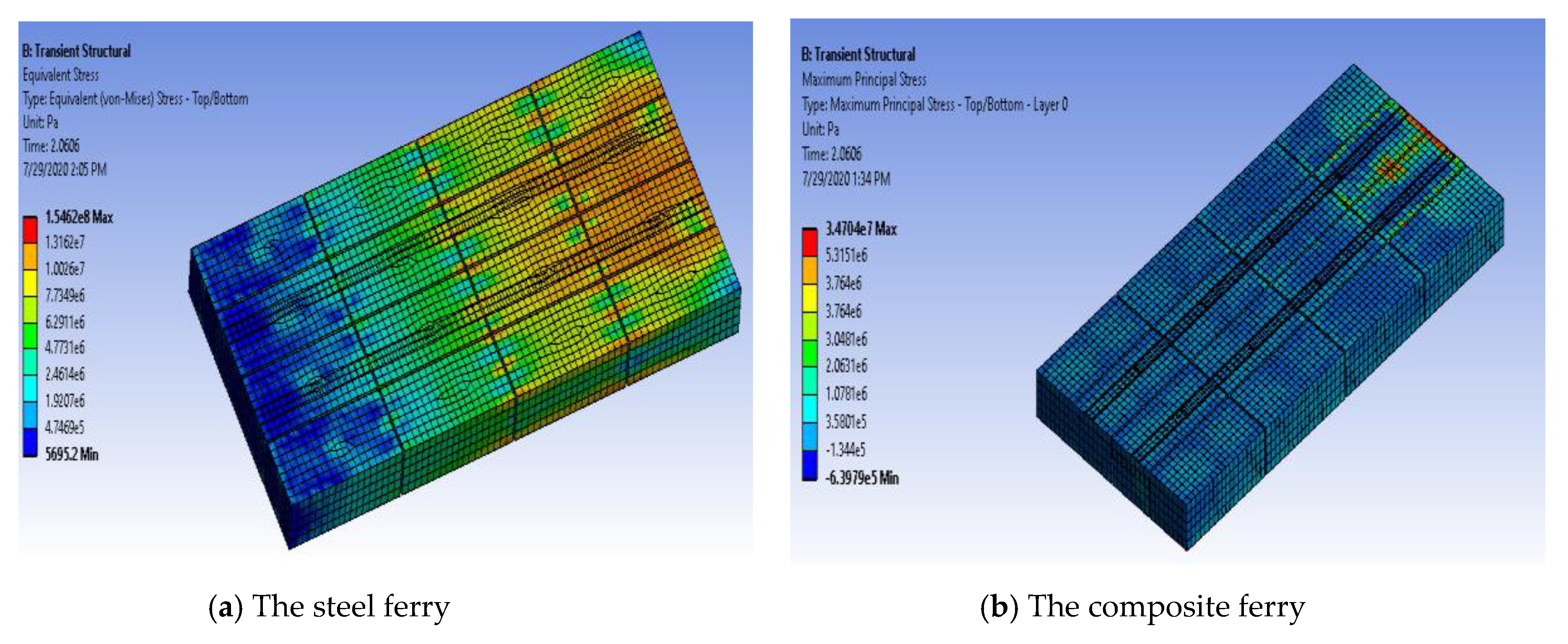
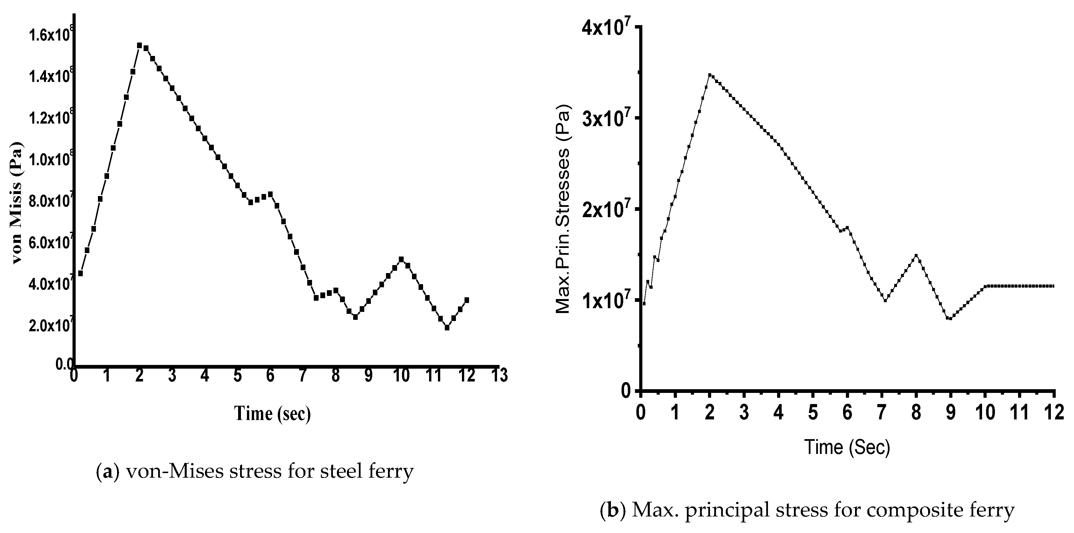
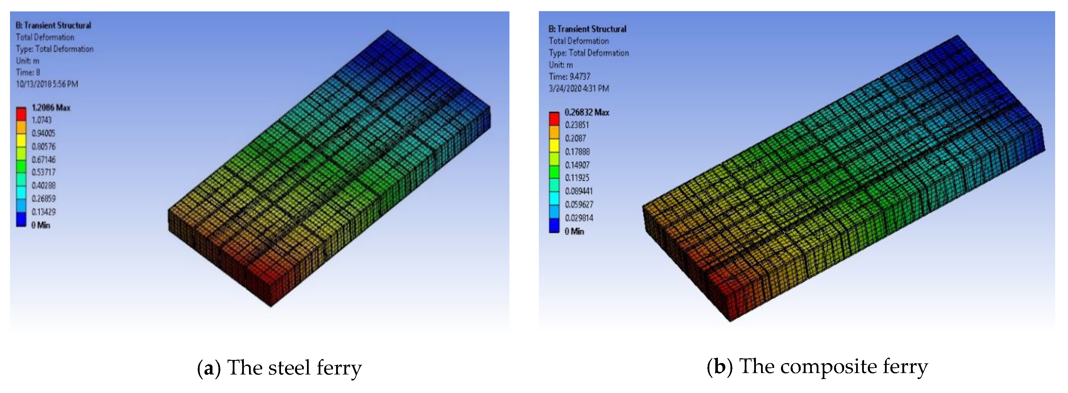
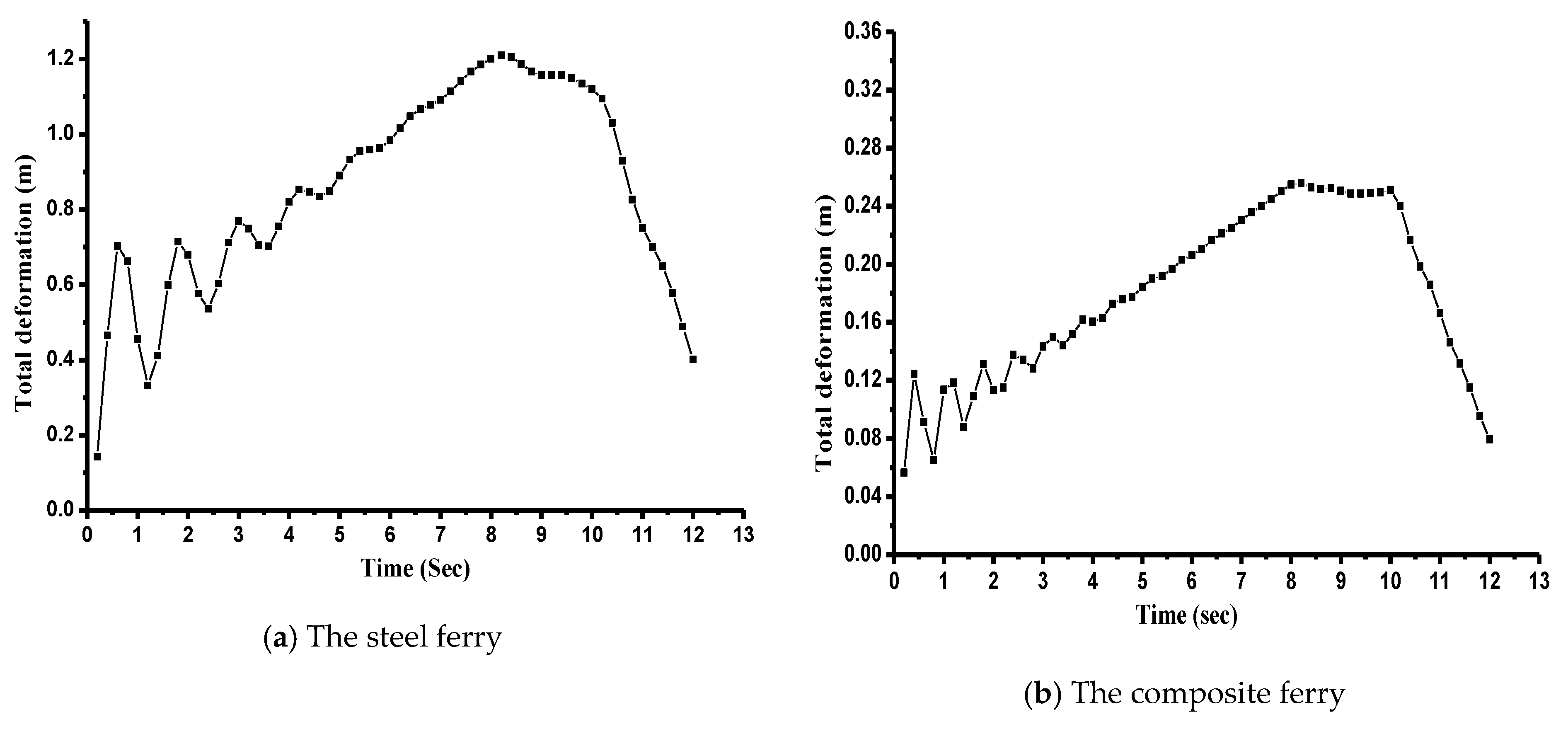
| Steel ferry | 562.5 | 1.1291 | 1.54 × | 1.2086 | 2.2 × | 1.262 | 1.58 × | 1.335 | 1.65 × |
| Comp. ferry | 153 | 0.2335 | 3.47 × | 0.2557 | 1.49 × | 0.279 | 1.62 × | 0.3034 | 2.078 × |
© 2020 by the authors. Licensee MDPI, Basel, Switzerland. This article is an open access article distributed under the terms and conditions of the Creative Commons Attribution (CC BY) license (http://creativecommons.org/licenses/by/4.0/).
Share and Cite
Lotfy, M.N.; Khalifa, Y.A.; Dessouki, A.K.; Fathallah, E. Dynamic Behavior of Steel and Composite Ferry Subjected to Transverse Eccentric Moving Load Using Finite Element Analysis. Appl. Sci. 2020, 10, 5367. https://doi.org/10.3390/app10155367
Lotfy MN, Khalifa YA, Dessouki AK, Fathallah E. Dynamic Behavior of Steel and Composite Ferry Subjected to Transverse Eccentric Moving Load Using Finite Element Analysis. Applied Sciences. 2020; 10(15):5367. https://doi.org/10.3390/app10155367
Chicago/Turabian StyleLotfy, Mohamed N., Yasser A. Khalifa, Abdelrahim K. Dessouki, and Elsayed Fathallah. 2020. "Dynamic Behavior of Steel and Composite Ferry Subjected to Transverse Eccentric Moving Load Using Finite Element Analysis" Applied Sciences 10, no. 15: 5367. https://doi.org/10.3390/app10155367
APA StyleLotfy, M. N., Khalifa, Y. A., Dessouki, A. K., & Fathallah, E. (2020). Dynamic Behavior of Steel and Composite Ferry Subjected to Transverse Eccentric Moving Load Using Finite Element Analysis. Applied Sciences, 10(15), 5367. https://doi.org/10.3390/app10155367