Machine-Learning Based Optimal Seismic Control of Structure with Active Mass Damper

Abstract

In recent years, optimal control which minimizes a cost function formulated by weighted states and control inputs has been applied to the seismic control of structures. Optimal control requires structural states which may not be available in real application; therefore, state estimation is essential, which inevitably takes additional computation time. However, time delay and state estimate error could affect the control performance. In this study, a multilayer perceptron (MLP) model and an autoregressive with exogenous inputs (ARX) model in machine learning are applied to learn the control force generated from a linear-quadratic regulator (LQR) with weighting matrices optimized by applying symbiotic organisms search algorithm. A 10-story building is adopted as a benchmark model for training and validation of the MLP and ARX models. Numerical simulation results demonstrate that the MLP and ARX models are able to emulate the LQR control force from the acceleration response directly, indicating that state estimation is not essential for optimal control implementation in real application. Finally, the machine-learning based approach is experimentally validated by conducting shake table testing in the laboratory in which the structural model is controlled by an active mass damper. The experimental results and structural control performance of the MLP and ARX models are compared with those of the LQR with a Kalman filter.

1. Introduction

Structural control systems have been extensively applied to suppress vibration responses of structures subjected to dynamic loads, particularly earthquake excitation. Modern structural control systems can be divided into passive control, active control, semi-active control, and hybrid control systems according to the characteristics of control devices and approaches [1]. Among the four strategies, active control is able to adapt structural response to take control actions to the structure during dynamic loads. Therefore, structures with active control application are mostly referred to as smart structures which can regulate structural response within the linear range and reduce or eliminate structural damage after strikes of earthquakes. For the realization of active control, two critical issues must be considered. The first issue is a structural control algorithm that is robust and clear enough to compute the control force to be imposed on the structure in real time. The other issue is an actuator controller that is able to apply the desired control force to the structure with acceptable tracking error in real time.

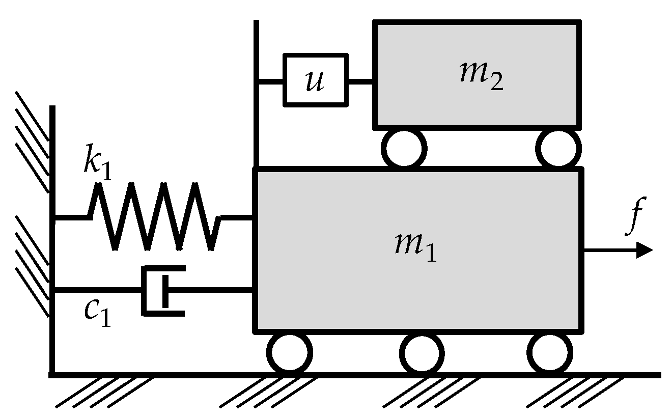
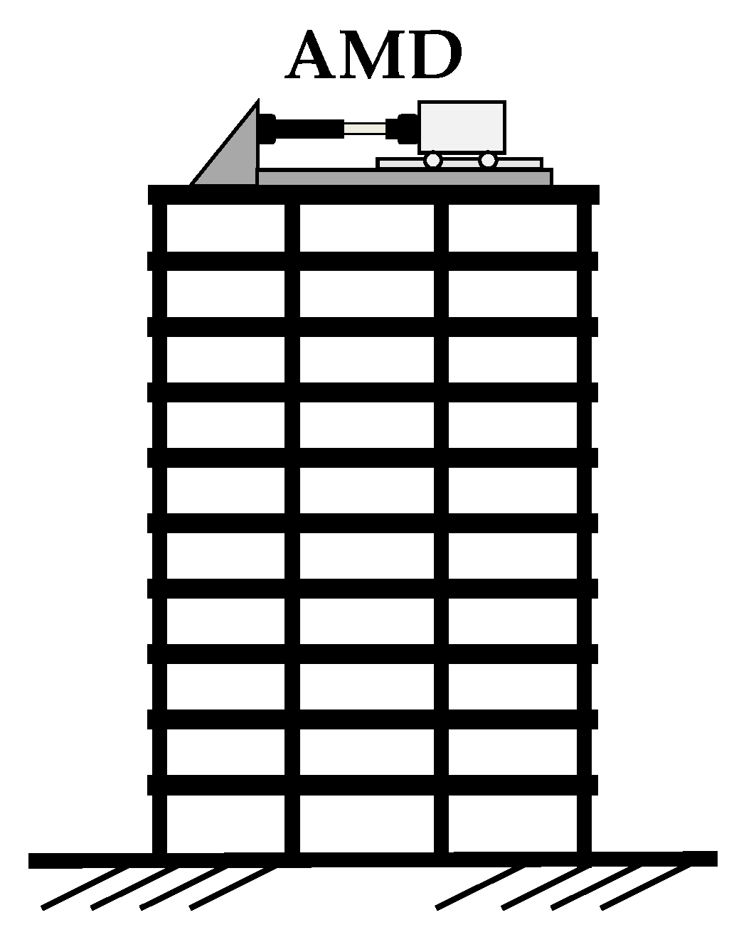
1.1. Active Mass Damper

An active mass damper (AMD)—which connects a moving mass block to the structure to be controlled through a hydraulic actuator—has been applied to mitigate vibration responses due to dynamic loads. The hydraulic actuator of an AMD system aims to reproduce desired force computed from the structural control algorithm through generating acceleration response of the mass block. Herein, the accuracy of the achieved control force is related to the acceleration control performance of the movement of the AMD mass block. Figure 1 illustrates the mathematical model of a building with an active mass damper in which m₁, c₁, and k₁ represent the mass, damping coefficient, and stiffness of the primary structure; m₂ is the mass of the AMD mass block; u is the control force; and f is the equivalent external force. Numerous studies have been focused on controller synthesis and analysis for computing desired force for AMD installed on a structure for the past decades. Various control algorithms for AMD have been proposed and validated such as the complete-feedback control algorithm which incorporates displacement, velocity and acceleration measurements as the feedback signal [2]; the linear-quadratic regulator (LQR) which requires displacement and velocity feedback [3]; and the linear-quadratic Gaussian (LQG) controller with acceleration feedback control [4,5]. Meanwhile, the neural network has been proposed and become an alternative to replace the control algorithm for structural control [6]. Chen et al. used the back-propagation algorithm proposed by Rumelhart et al. [7] for training neural network in structural control [8]. Bani-Hani and Ghaboussi applied the neural network control algorithm to a nonlinear three degrees-of-freedom steel frame model [9]. Kim et al. proposed an optimal control algorithm using neural networks through minimization of the cost function [10]. Hung et al. used neural networks with a training algorithm for active pulse structural control without the trial-and-error selection of the learning rate [11]. Cho et al. applied a neural network control for nonlinear bridge systems with earthquake excitation [12]. Lin et al. proposed a smart active control framework which utilized fiber Bragg grating sensors and neural networks [13]. In addition, the neural network controller has been applied to reduce the wind-induced vibration of a tall building through an active tuned mass damper [14]. An AMD controller used neural network based on optimal control method for a cable-stayed bridge structure [15]. Most of these studies have been focused on numerical simulation without experimental validation. Recently, Chen and Yang [16] proposed a neural network with modified Newton method for structural control with an AMD and validated the control performance through shake table testing. Experimental results have shown that the neural network controller is effective in damping control applications. However, the mass ratio of the AMD used in the experiment was more than 20% which is not realistic in real implementation for buildings. Practical experimental studies regarding to the AMD seismic control performance achieved by using machine learning are considered limited.

1.2. Motivation

LQR has been considered one of the most effective controllers for structural control; however, it requires structural states for feedback which may not be measurable in real application. As a result, a state observer or estimator is necessary which could increase the computational effort and lead to time delay in the control loop. Furthermore, state estimation error could reduce the control performance or even lead to inferior structural response. Last but not least, control performance of LQR depends on the weighting matrices in the cost function. Well-determined weighting matrices lead to effective control performance with limited force capacity of active devices. Therefore, the objectives of this study are (1) to optimize the weighting matrices of LQR that leads to effective control performance; (2) to replace the LQR with a controller that intends to emulate the control performance of the LQR without a state estimator; and (3) to demonstrate the control performance of the LQR and the controllers that emulate the LQR through numerical and experimental approaches. In this study, machine learning-based control models are proposed and trained to emulate an LQR with weighting matrices optimized by applying a novel and simple metaheuristic algorithm named symbiotic organisms search (SOS). A 10-story benchmark building controlled by an AMD is adopted for numerical studies. The AMD is controlled by an LQR in the modal configuration optimized by the SOS with respect to the objective function considering the square root of sum of squares (SRSS) of maximum acceleration of the selected modes. The LQR with optimized weighting matrices is expected to achieve effective seismic control performance, which, however, may be affected by the performance of state estimator. As a result, two neural network models are adopted for data training including the multilayer perceptron (MLP) model and the autoregressive with exogenous inputs (ARX) model to emulate the control performance of LQR. However, state estimation is not critical in the neural network models which reduces the effect of state estimation error on the seismic control performance of LQR. Afterwards, the numerical simulation results are compared and discussed thoroughly. Finally, shake table testing is performed for experimental validation in the structural laboratory and the results are summarized and concluded.

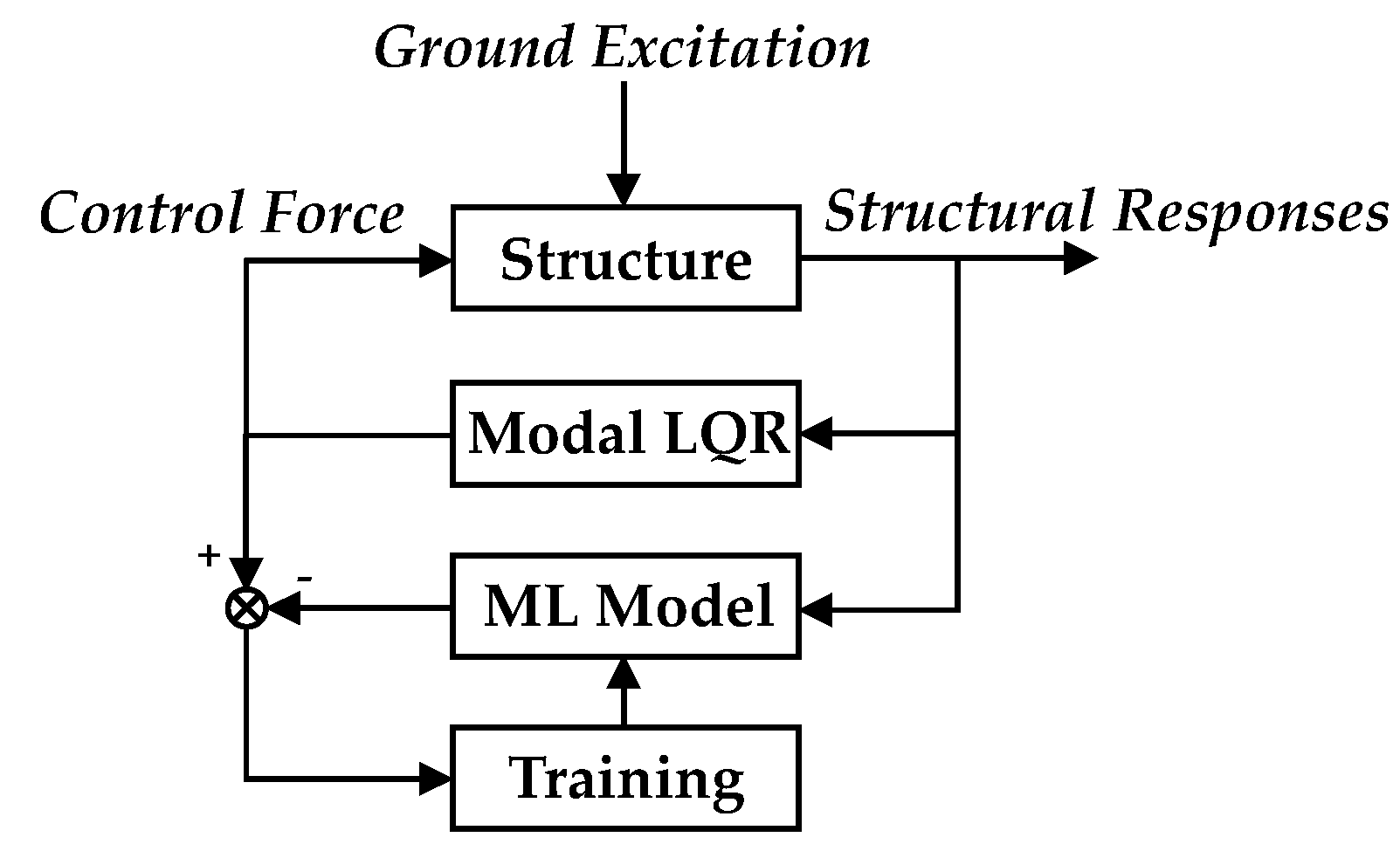
2. Modal LQR with Optimized Weighting Matrices

LQR minimizes a cost function related to weighted states and control inputs. However, it is not straightforward to tune the weighting matrices in the cost function for designing the LQR. Generally, the weighting matrices are determined by trial and error which could lead to limited seismic control performance. Therefore, optimization of LQR weighting matrices has become a research topic recently. In particular, metaheuristic optimization algorithms have been applied to determine the weighting matrices of LQR with respect to user-defined objective functions. For completeness, the optimization procedure of LQR weighting matrices in modal configuration is introduced briefly.

2.1. Modal LQR

Consider a N-degrees-of-freedom building with an AMD at the top, its equations of motion can be expressed as:

$$M\ddot{x}(t)+C\dot{x}(t)+Kx(t)=-Ml{\ddot{x}}_g(t)+\Lambda u(t)$$

(1)

where M, C, and K represent the mass, damping, and stiffness matrix of the building, respectively; x(t) is the displacement vector; u(t) is the control force; Λ is the location vector of the control force; l is a vector of order N with each element equal to unity; and ${\ddot{x}}_g(t)$ is the ground acceleration. It is noted that proportional damping of structures has been frequently assumed in structural dynamic analyses. As a result, if the building is proportional damping system, the equation of motion can be expressed in modal configuration by letting $x(t)=\Phi q(t)$. Hence, the equation of motion in modal space becomes:

$$\ddot{q}(t)+\overline{C}\dot{q}(t)+{\Omega }^{2}q(t)=-{\Phi }^{T}Ml{\ddot{x}}_g(t)+{\Phi }^T\Lambda u(t)$$

(2)

where Φ is the modal matrix which contains all the mode shapes; q(t) is the modal displacement vector; $\overline{C}=diag\left(\begin{array}{ccc}2{\zeta }_1{\omega }_1& \cdots & 2{\zeta }_N{\omega }_N\end{array}\right)$ is a modal damping matrix in which the parameters ζ_i and ω_i represent the damping ratio and natural frequency of the i-th mode, respectively; and Ω² is the modal natural frequency matrix and can be expressed as ${\Omega }^2=diag\left(\begin{array}{ccc}{\omega }_1^2& \cdots & {\omega }_N^2\end{array}\right)$. The state-space formulation of the building in modal space can be represented as:

$$\begin{array}{l}{\dot{z}}_m(t)=A_m{z}_m(t)+B_{m}u(t)+E_m{\ddot{x}}_g(t)\\ y_m(t)=C_m{z}_m(t)+D_{m}u(t)\end{array}$$

(3)

where ${\dot{z}}_m(t)={\left[\begin{array}{cc}q(t)& \dot{q}(t)\end{array}\right]}^T$ defines the modal states. Accordingly, the system matrix A_m, the control force distribution matrix B_m, and the disturbance location matrix E_m in modal configuration become

$$A_m=\left[\begin{array}{cc}0& I\\ -{\Omega }^2& -\overline{C}\end{array}\right];B_m=\left[\begin{array}{c}0\\ {\Phi }^T\Lambda \end{array}\right];E_m=\left[\begin{array}{c}0\\ -{\Phi }^{T}Ml\end{array}\right]$$

(4)

On the other hand, the output y_m(t) is selected as the modal absolute acceleration of each mode and the matrices C_m and D_m become:

$$C_m=\left[\begin{array}{cc}-{\Omega }^2& -\overline{C}\end{array}\right];D_m=\left[{\Phi }^T\Lambda \right]$$

(5)

As mentioned previously, LQR intends to minimize a cost function related to the states and control inputs with weighting matrices Q and R determined by users. In the modal LQR design, the modal absolute acceleration is taken as the state to be regulated. Therefore, the quadratic cost function of LQR for structural control is defined as:

$$J={\displaystyle {\int }_0^{\infty }\left(y_m{}^{T}Q{y}_m+u^{T}Ru\right)\mathrm{d}t}$$

(6)

The dimension of the weighting matrix Q depends on the number of selected modes to be controlled. The weighting R is a scalar since there is merely one control force imposed on the top of the structure. The state feedback gain matrix K_m can be obtained by solving the Ricatti equation:

$$K_m=R^{-1}{B}_m{}^{T}P$$

(7)

where P is the solution of the Ricatti equation:

$$A_m{}^{T}P+P{A}_m-P{B}_m{R}^{-1}{B}_m{}^{T}P+C_m{}^{T}Q{C}_m=0$$

(8)

The control force for modal LQR control becomes u(t) = −K_mz_m(t). In order to convert the control input from the modal space to the configuration space, the gain matrix K_m needs to be converted into K_g through:

$$K_g=K_m\left[\begin{array}{cc}{\Phi }^{-1}& 0\\ 0& {\Phi }^{-1}\end{array}\right]$$

(9)

Accordingly, the state feedback gain matrix K_g can be used to calculate the control force for the structure by u(t) = −K_gz(t) where z is the states in the configuration space which contains the displacement and velocity vectors, i.e., $\dot{z}(t)={\left[\begin{array}{cc}x(t)& \dot{x}(t)\end{array}\right]}^T$.

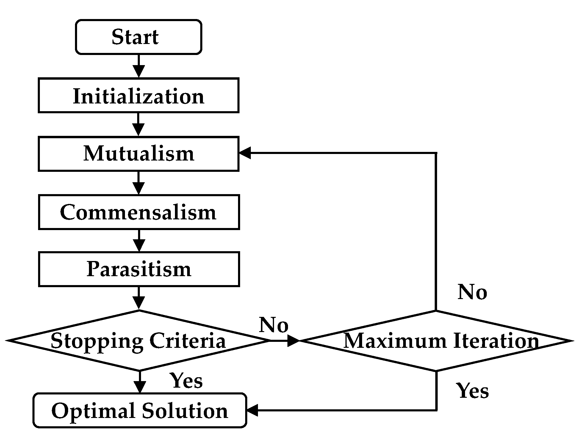
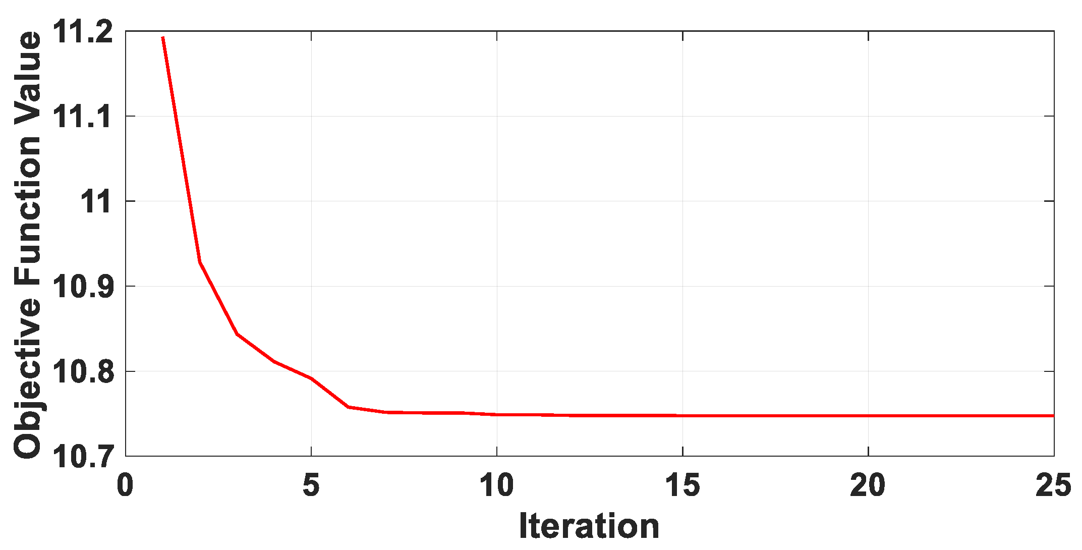
2.2. Symbiotic Organisms Search

Symbiotic Organisms Search (SOS), proposed by Cheng and Prayogo [17], is a novel metaheuristic optimization algorithm which emulates the interactive behavior among organisms in nature with three phases, namely mutualism, commensalism, and parasitism. Figure 2 shows the simplified flowchart of SOS procedure. In the initialization, each organism is assigned random location in the n-th dimensional search space where n represents the number of parameters to be optimized. The fitness of each organism with respect to the objective function is evaluated and the one with the best fitness value is recorded as x_best. In the mutualism phase, two organisms are randomly selected and the position of each organism is updated by following the equation:

$${x_i}^{\prime }=x_i+rand(0,1)\cdot (x_{best}-\frac{x_i+x_j}{2}\cdot B{F}_1);{x_j}^{\prime }=x_j+rand(0,1)\cdot (x_{best}-\frac{x_i+x_j}{2}\cdot B{F}_2)$$

(10)

where x_i’ and x_j’ are the updated position of the i-th and j-th organisms, respectively; and BF₁ and BF₂ are the benefit factors of the i-th and j-th organisms, respectively which are randomly assigned as either 1 or 2 at each iteration step. The benefit factors are utilized to simulate whether the two organisms partially or fully benefit from the other. Since BF₁ and BF₂ are randomly assigned, tuning is not required in the mutualism phase. The commensalism phase is performed after the mutualism phase is completed. Similar to the mutualism phase, two organisms are randomly selected and one of them intends to benefit from the other by:

$${x_i}^{\prime }=x_i+rand\left(-1,1\right)\cdot (x_{best}-x_j)$$

(11)

Finally, the parasitism phase is conducted after the commensalism phase is completed. A parasite organism is created by duplicating an organism which is picked randomly and modifying the arbitrarily selected dimensions using a random number. Then, another organism is selected randomly from the ecosystem as the host to be attacked by the parasite organism. The fitness values of the parasite and the host are both evaluated. If the fitness value of the parasite organism is better than that of the host, the parasite organism kills the host organism and assumes its position in the ecosystem. On the contrary, if the parasite does not have a better fitness value, it is terminated immediately. Consequently, the mutualism, commensalism, and parasitism phases work in sequence until the predefined number of iteration steps is reached.

3. Neural Network Models

In this study, a machine-learning based controller is aimed to replace the modal LQR in the control loop. The structural responses controlled by the modal LQR is used as input of the model and the control force generated by the modal LQR is the output of the model. Machine learning (ML) is used to train the input-output relationship of the model as illustrated in Figure 3. Since the structural responses and control force are time series data, two artificial neural network models are adopted for training in this study. Artificial neural networks (ANN) are biologically inspired computational networks based on studies of the brain and nervous system. Processing elements named as neurons or perceptrons are arranged in a layer with the output of one layer becoming the input to the neurons in the next layer. The entire neural network transfers the input signals to output signals through layers of neurons with various weightings and activation functions.

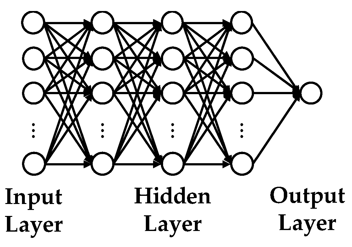
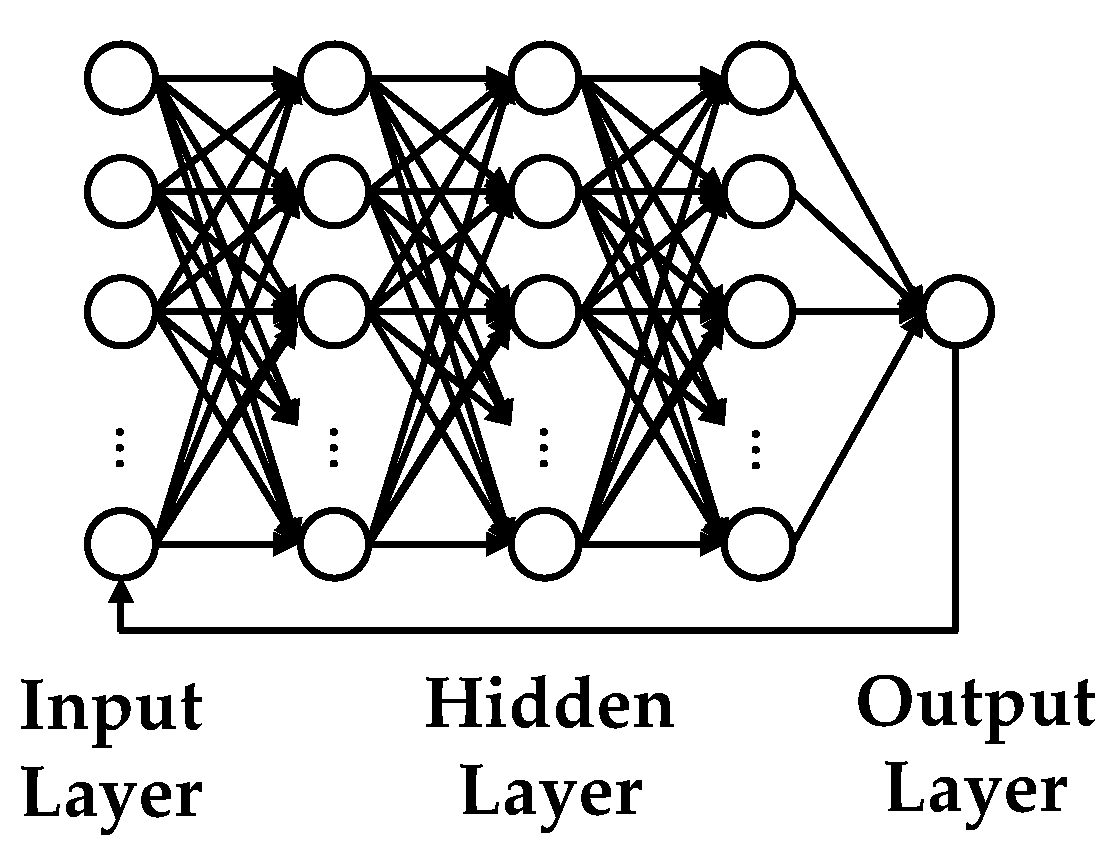
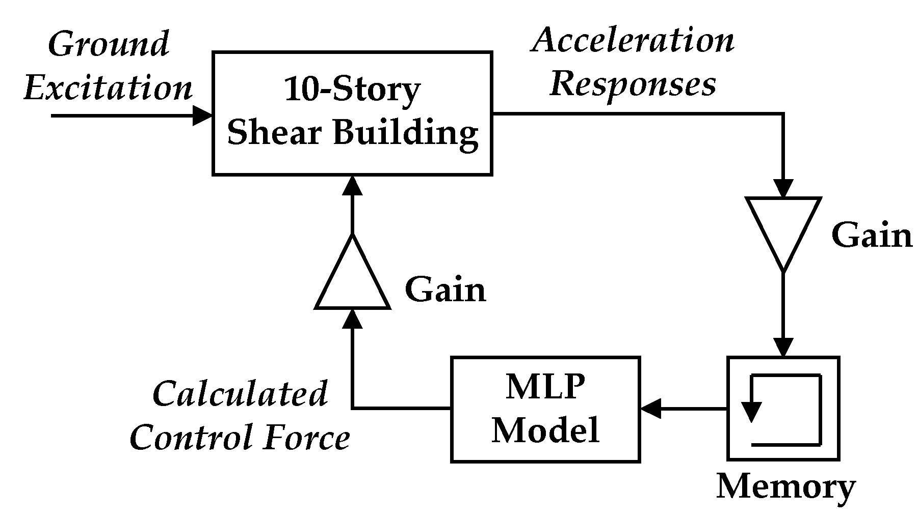
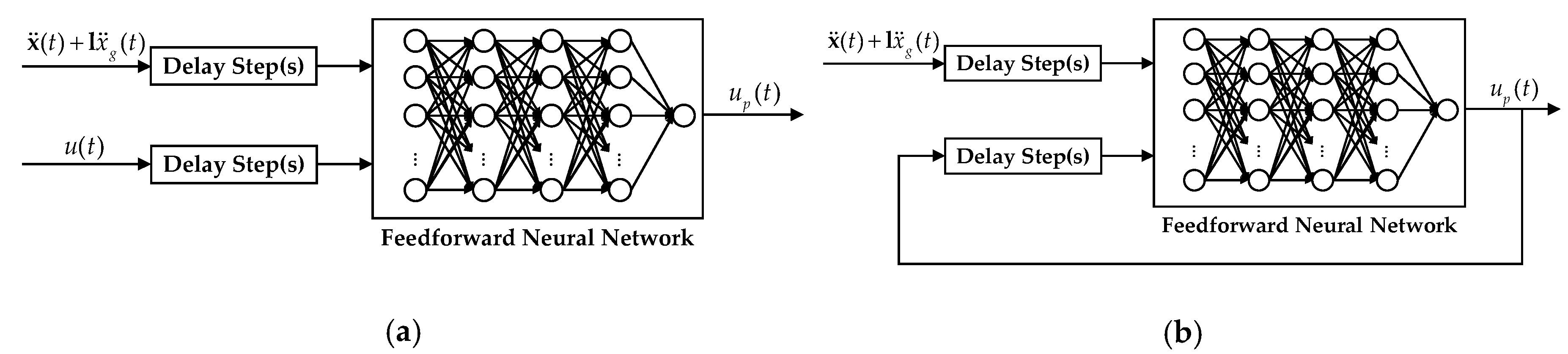
3.1. Multilayer Perceptron Model

Multilayer perceptron (MLP) is a supervised learning algorithm that learns a function from inputs to outputs. Generally, an MLP model is composed of an input layer, an arbitrary number of hidden layers, and an output layer as depicted in Figure 4. Each neuron converts the weighted sum of inputs into an output using an activation function which can be either linear or nonlinear. The MLP network is used frequently in time series prediction as it is able to learn nonlinear models, and support multiple input with online learning. In this study, the input of the MLP model is the structural acceleration responses at each floor with previous multiple time steps while the output is the control force of the AMD at the predicting step.

3.2. Autoregressive Exogenous with Exogenous Inputs Model

An autoregressive with exogenous inputs (ARX) model, which is a recurrent dynamic neural network has been used in various applications of time-series modeling. In the ARX architecture as shown in Figure 5, the predicted output is performed from the present and past values of input as well as the past predicted values. In this study, the input of the ARX model is the structural acceleration responses at each floor with previous multiple time steps and the control force at the previous step. The output is the control force of the AMD at the predicting step. Since an ARX model requires output as input, it is considered as a recurrent neural network model.

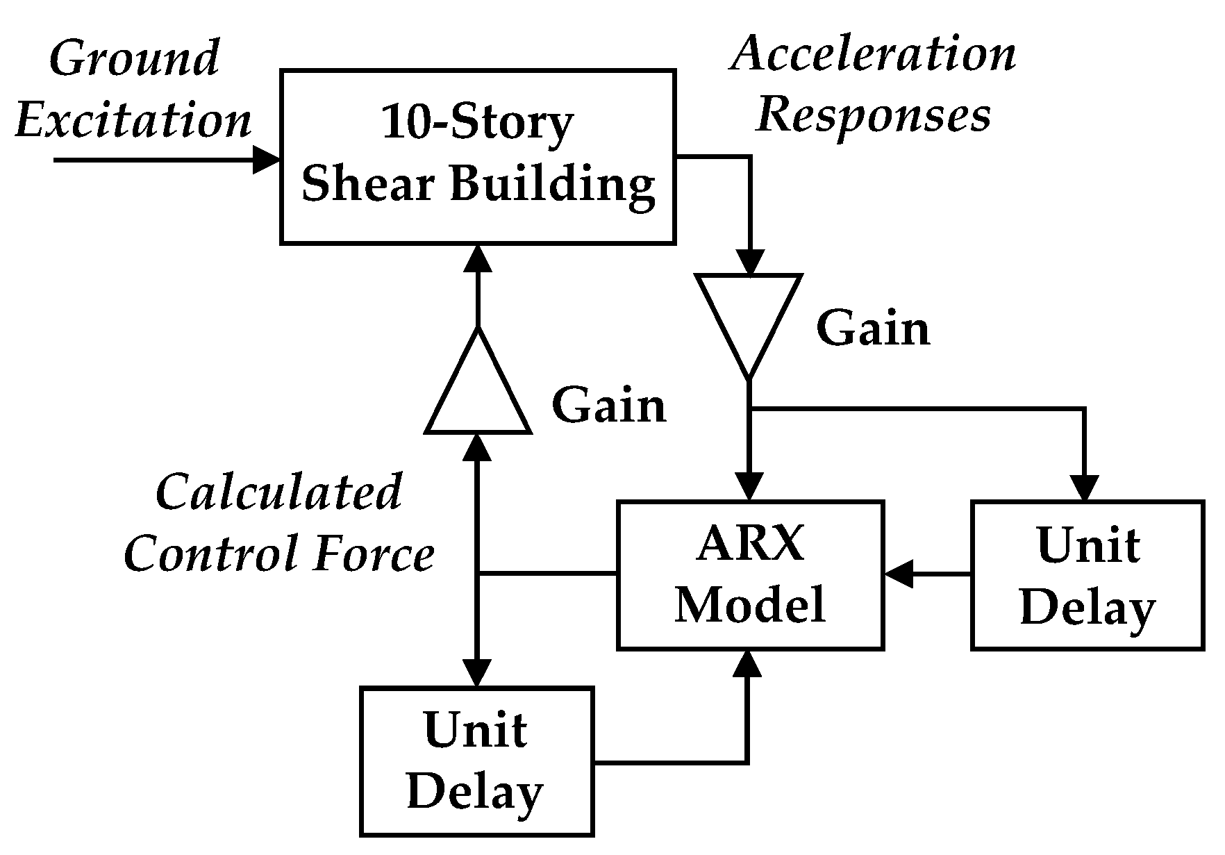
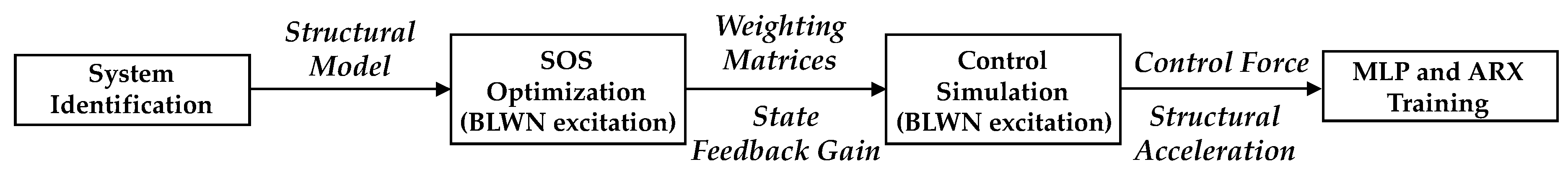
4. Numerical Study: A 10-Story Shear Building

4.1. Modal LQR with Optimized Weighting Matrices

A 10-story shear building used by Amini et al. [18] was adopted as a benchmark structural model for training and validation of the machine-learning based control, which was aimed to replace the modal LQR in the control loop. The mass and the stiffness of each story of the shear building were 10 kN-s²/m and 2000 kN/m, respectively. The undamped natural frequencies of the first five modes of the structure are shown in

Table 1. Natural frequencies of the benchmark structural model (Hz).

1st Mode	2nd Mode	3rd Mode	4th Mode	5th Mode
0.336	1.002	1.644	2.250	2.807

. An active mass damper was assumed to be installed on the top floor of the structural model with a force capacity of ±50 kN, which was roughly equal to 5% structural weight. The damping ratio of the structural model was assumed 2% for all vibration modes. Figure 6 depicts the schematic of the 10-story shear building with an AMD at the top.

For modal LQR control approach, the number of control modes need to be determined first. In this study, the effective modal mass was adopted to determine the number of control modes because it provided a straightforward approach for assessing the importance of each vibration mode. It is known that the effective modal mass can be interpreted as part of the total mass of a structure responding to an earthquake in each mode which is associated with natural frequencies and mode shapes. Merely the modes which have significant effective modal masses are critical to represent the structural response in a certain frequency range. The selection strategy was that the accumulated effective modal mass of the selected control modes must be larger than 95% of the total mass of the structure. Since the effective modal mass of the 1st, 2nd, and 3rd mode was 84.79 kN-s²/m, 9.14 kN-s²/m, and 3.09 kN-s²/m, respectively, the accumulated effective modal mass of the first three modes were 97.02 kN-s²/m which was larger than 95% of the structural weight (95 kN-s²/m). As a result, the first three modes were adopted as the control modes in the numerical study. MATLAB/Simulink, provided by The Mathworks Inc., Natick, MA, USA was adopted to conduct the numerical simulation of the 10-story building with AMD optimized by SOS with respect to the objective function:

$$\sqrt{\max \left[y_{m1}{\left(t\right)}^2\right]+\max \left[y_{m2}{\left(t\right)}^2\right]+\cdots +\max \left[y_{m{n}_m}{\left(t\right)}^2\right]}$$

(12)

where y_mi represents the modal acceleration of the i-th mode; and n_m is the number of control modes. Actually, the objective function is the SRSS of maximum acceleration of the selected modes. For the optimization of weighting matrices, the weighting R was remained a fixed value of 100 while 10¹⁰ and 0 were selected as the upper and lower bounds value of each element in the weighting marix Q. A band-limited white noise (BLWN) with a peak ground acceleration (PGA) of 2.4 m/s², a bandwidth from 0 Hz to 15 Hz, and a duration of 140 s was used to excite the 10-story shear building. The root-mean-square (RMS) of the BLWN was 0.5526 m/s². The bandwidth was considered sufficient to cover the frequency component of most historical earthquake. It is worth noting that saturation with 10% of the actuator capacity of AMD was used in the optimization because the generated force of the LQR could reach the force capacity of the AMD actuator without the 10% saturation. A number of 100 organisms and 35 iterations were adopted for SOS optimization. Figure 7 depicts the convergence curve with respect to the objective function. It shows that the optimal value was reached at the 11th iteration. Note that the initial values in the weighting matrix Q were randomly assigned; however, the corresponding LQR still achieved effective control performance. After the first iteration, the objective function value was significantly reduced. Finally, the corresponding optimized state feedback gain matrix K_g was obtained as:

$$\begin{array}{l}{K}_g=[38.0559.8857.0532.71-0.47-27.04-36.66-28.85-12.420.18\\ 5.635.89-1.17-12.62-21.96-22.60-11.648.1429.1742.61]\end{array}$$

(13)

Note that the control force is calculated by multiplying the state feedback gain matrix by the states of the 10-story shear building. The states of the 10-story shear building can be directly obtained without noise or distortion in the numerical simulation. However, the states of a structure to be controlled are not always measurable in real practice. Thus, an observer or a state estimator such as the Kalman filter is essential.

4.2. Training and Validating of MLP Model

In this study, Keras, a high-level neural networks application programming interface written in Python, was used as the framework for programming. TensorFlow was adopted as the backend engine for Keras which is compatible with most of the processors available in the marketplace. As a result, Keras was executing on top of TensorFlow providing a quick and efficient approach for neural-network training. For the software version used in this study, the Python version was 3.7.4; Tensorflow version was 1.14; Keras version was 2.3.1; and the CUDA version for GPU accelerated applications was 10.0. Furthermore, Intel Core i7-9700 with Windows 10 operating system and NVIDIA RTX-2080 Super graphics card were used for the hardware devices.

The MLP model is a fully connected feedforward model. In this study, the MLP with a linear activation function was adopted as the 10-story shear building was linear. The state feedback gain matrix K_g shown in Equation (13) was used in the time history analysis of the 10-story shear building with an AMD at the roof subjected to a BLWN ground acceleration. The corresponding absolute acceleration of each floor was taken as the input of the MLP model and the generated control force was the desired output to be predicted by the MLP model. In the training process, the MLP model with one input layer, three hidden layers, and one output layer was structured. Each hidden layer contained 300 neurons. The output layer had merely one neuron representing the control force at the current predicting step. Since the control force at the current step was related to previous various steps of structural response, the number of neurons in the input layer was investigated first in the study. Note that the acceleration and control force from the time history analysis were normalized to a peak value of ±1.0 before the training process of MLP was conducted. The objective of training the MLP aims to optimize the weights of the model; therefore, a loss function was required for training. In this study, the mean square error (MSE) between the predicted and desired control force was adopted as the loss function. The adaptive moment estimation (Adam) optimizer [19] which computed adaptive learning rates for each parameter was used to train the model in addition to the characteristics of adaptive gradient descent. Since the calculation of Adam included offset correction, the weight updating of the MLP model was sustained within a specific range. As a result, the update of parameters was relatively smooth and the calculation efficiency was exceptional.

As mentioned previously, the number of acceleration steps for training was investigated as a parametric study in order to confirm the appropriate number of neurons in the input layer. The number of epochs in the parametric study was selected 5000. The learning effectiveness of the MLP model was evaluated by calculating the root-mean-square error (RMSE) between the desired and predicted control force which can be expressed as:

$$\mathrm{RMSE}(\%)=\sqrt{\frac{{\displaystyle \sum _{k=1}^N{\left(u[k]-u_p[k]\right)}^2}}{{\displaystyle \sum _{k=1}^{N}u{[k]}^2}}}\times 100\%$$

(14)

where u[k] and u_p[k] are the desired and the predicted control force at the kth step, respectively. It is realized that better learning leads to smaller RMSE. After training, the MLP model was then implemented in the control simulation model as shown in Figure 8 using MATLAB/Simulink. The input of the MLP was the acceleration response of each floor with the current and previous steps, and the output was the calculated control force imposed on the 10-story shear building. Note that the training data of acceleration and control force for MLP were normalized to a peak value of ±1.0; therefore, the acceleration responses of the building were scaled by a gain before they were input to the MLP model. Similarly, the calculated control force of the MLP model was also scaled before it was imposed on the shear building.

Table 2. Training results considering various acceleration steps for the multilayer perceptron (MLP).

Number of Acceleration Steps
	10	50	100	120	150	200
Training RMSE (%)	1.95	0.40	0.62	0.68	0.89	0.87
Simulation RMSE (%)	N.A.	N.A.	N.A.	1.77	1.82	1.70

shows the training results considering various number of acceleration steps in the input layer. It can be found that the RMSE between the desired and predicted control force is smaller than 2.0% for all cases, indicating that the MLP model is able to learn the control force generated from an LQR with optimized weighting matrices through the corresponding controlled acceleration responses. Thus, it was expected that the implementation of the MLP model as depicted in Figure 8 should be able to generate similar control force to the LQR control force. The ode5 solver using the Dormand–Prince formula was adopted for the control simulation in Simulink. Table 2 also shows the RMSE between the desired and predicted control force in the control simulation model. All the simulations were computed using a sampling rate of 200 Hz. However, the control simulation model was divergent and became inexecutable for the cases of 10, 50, and 100 acceleration steps due to error propagation in the control loop. On the other hand, the cases of 120, 150, and 200 acceleration steps all led to stable and satisfactory simulation results. Among the three successful cases, the computational effort of the 120 steps was the least. Therefore, it was suggested that a minimum number of 120 steps was needed as the input of the MLP model. Accordingly, a minimum number of 1210 neurons was required in the input layer for the MLP model.

4.3. Training and Validating of ARX Model

Generally, training an ARX model can be categorized into series-parallel and parallel architectures as shown in Figure 9 which can be expressed as the two equations, respectively:

$$u_p[k]=f\left(\begin{array}{cccc}\ddot{x}[k]+l{\ddot{x}}_g[k],& \ddot{x}[k-1]+l{\ddot{x}}_g[k-1],& \cdots & ,\ddot{x}[k-n_a]+l{\ddot{x}}_g[k-n_a],\\ u[k-1],& u[k-2]& \cdots & ,u[k-n_f]\end{array}\right)$$

(15)

$$u_p[k]=f\left(\begin{array}{cccc}\ddot{x}[k]+l{\ddot{x}}_g[k],& \ddot{x}[k-1]+l{\ddot{x}}_g[k-1],& \cdots & ,\ddot{x}[k-n_a]+l{\ddot{x}}_g[k-n_a],\\ u_p[k-1],& u_p[k-2]& \cdots & ,u_p[k-n_f]\end{array}\right)$$

(16)

where u[k] and u_p[k] are the desired and the predicted control force at the k-th step, respectively; and n_a and n_f are the number of acceleration and control force delay steps for training in ARX model. In the series-parallel architecture, the predicted control force u_p[k] is calculated from the current and previous steps of the absolute acceleration at each floor as well as the previous steps of the desired control force. In the parallel architecture, the predicted control force u_p[k] is performed from the present and past values of the absolute acceleration at each floor as well as the past predicted control force. In this study, the series-parallel architecture was adopted for training while the parallel architecture was implemented in the control simulation model of MATLAB/Simulink. In the training process, the ARX model with one input layer, two hidden layers, and one output layer was structured. The first and second hidden layer contained 100 and 50 neurons, respectively. In the output layer, there was simply one neuron representing the control force at the current step. The number of acceleration and control force delay steps in the training process were selected one, i.e., n_a = n_f = 1. Accordingly, the dimension of the ARX neural network model was 21 × 100 × 50 × 1. Similar to the MLP training, the training data of acceleration and control force were normalized to a peak value of ±1.0, and the MSE between the predicted and desired control force was used as the loss function and Adam was applied as the optimizer. The number of epochs was 5000. The RMSE between the desired and predicted control force was 0.25%.

After training, the ARX model was also implemented in the control simulation model using MATLAB/Simulink as illustrated in Figure 10. The simulation configuration for the ARX model was identical to that for the MLP model. The corresponding RMSE between the desired and predicted control force in the control simulation model was 4.90%. Note that the RMSE of the ARX training result was approximate to those of the MLP training results. However, the RMSE in the control simulation model of the ARX model was larger than those of the MLP model with 120, 150, and 200 acceleration steps. This is because the series-parallel architecture was used in the training process and it was replaced by the parallel architecture in the control simulation. It is worth noting that the elapsed time for training the ARX model was merely 90 s. However, it took more than 1.5 h for training the MPL model with 120 acceleration steps. This is attributable to that the dimension of the ARX model (21 × 100 × 50 × 1) was significantly smaller than those of the MPL models (1210 × 300 × 300 × 300 × 1 for the case with 120 acceleration steps).

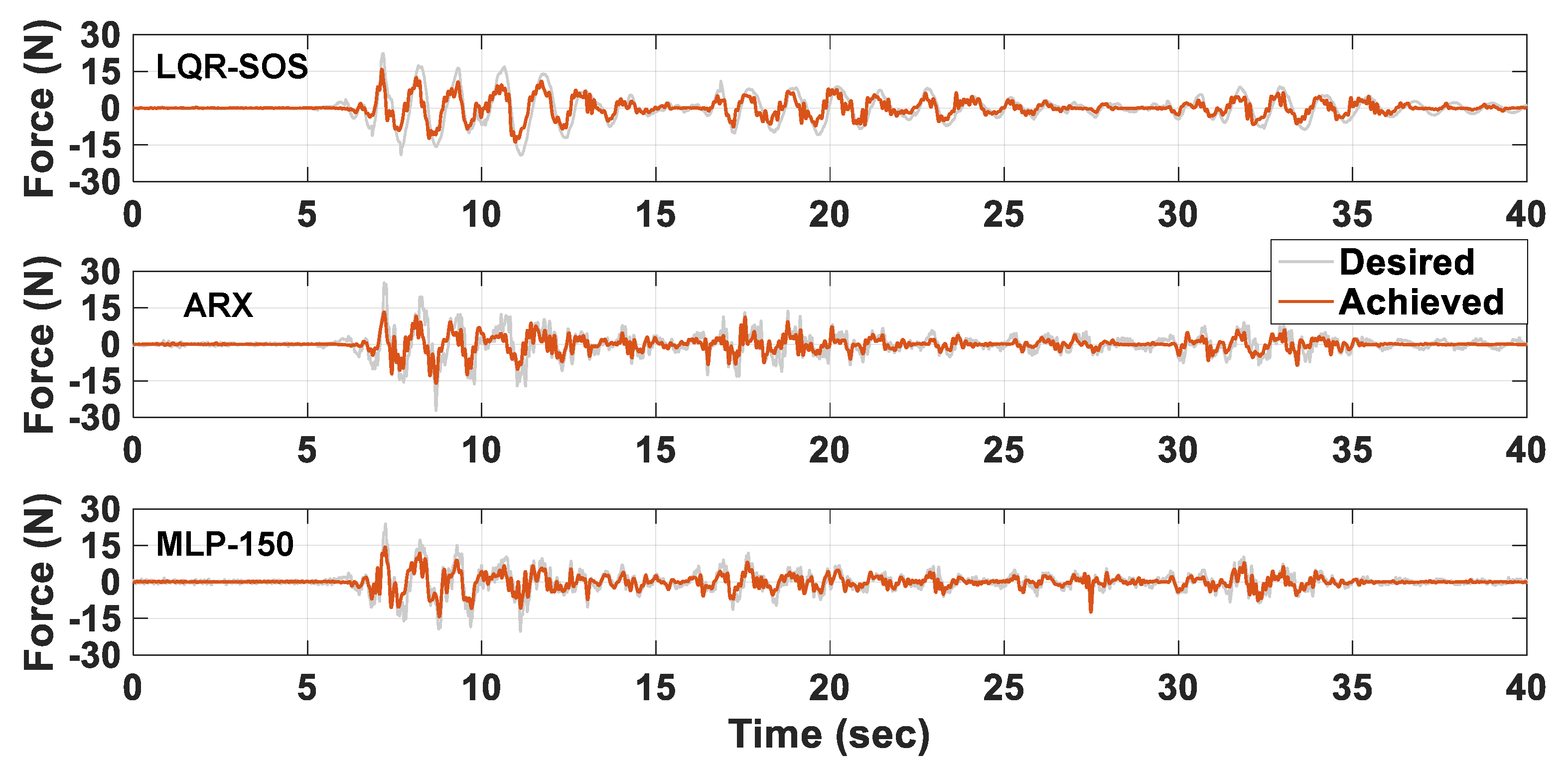
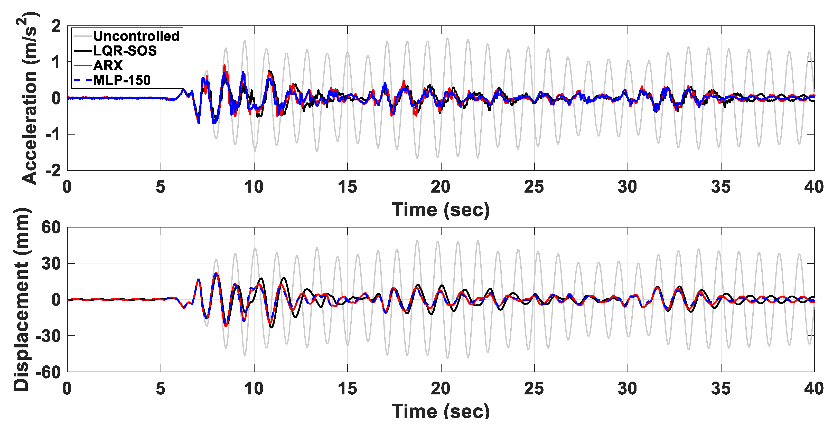
4.4. Comparison of Seismic Control Performance

In order to realize how accurately the MLP and ARX models were able to emulate the LQR, four of the performance indices used by Jansen and Dyke [20] were adopted. The first performance index denotes the maximum normalized floor relative displacement which can be expressed as:

$$J_1=\underset{t,i}{\max }\left(\frac{\left|x_i(t)\right|}{x^{\max }}\right)$$

(17)

where x_i(t) is the relative displacement of the i-th floor during the excitation; and x^max represents the maximum displacement of the uncontrolled shear building. The second performance index is the maximum normalized inter-story drift which can be represented as:

$$J_2=\underset{t,i}{\max }\left(\frac{\left|d_i(t)/h_i\right|}{d_n{}^{\max }}\right)$$

(18)

where d_i(t) is the inter-story drift of the i-th floor during the excitation; h_i is the story height of the i-th floor; and d_n^max represents the maximum normalized inter-story drift of the uncontrolled shear building. The third performance index is the normalized peak absolute acceleration which can be expressed as:

$$J_3=\underset{t,i}{\max }\left(\frac{\left|{\ddot{x}}_{ai}(t)\right|}{{\ddot{x}}_{ai}{}^{\max }}\right)$$

(19)

where ${\ddot{x}}_{ai}(t)$ is the absolute acceleration of the i-th floor during the excitation; and ${\ddot{x}}_{ai}{}^{\max }$ is the maximum absolute acceleration of the i-th floor of the uncontrolled shear building. The last performance index considers the maximum control force normalized by the weight of the structure which is formulated as:

$$J_4=\underset{t}{\max }\left(\frac{\left|u(t)\right|}{W}\right)$$

(20)

where u(t) is the control force of AMD and W is the weight of the 10-story shear building.

Fourteen earthquake ground acceleration records normalized to a PGA of 2.4 m/s² were adopted as the ground excitation to the 10-story shear building with an AMD. The AMD control force was generated by using the LQR state feedback control with optimized weighting matrices using SOS (LQR-SOS), the MLP models with 120, 150, and 200 input acceleration steps (MLP-120, MLP-150, and MLP-200), and the ARX model. As mentioned previously the force capacity of the AMD was assumed ±50 kN. The AMD controlled 10-story shear building was subjected to the fourteen earthquakes.

Table 3. Seismic control performance of the LQR (linear-quadratic regulator) -SOS (symbiotic organisms search).

Earthquakes	J1	J2	J3	J4
El Centro	0.434	0.523	0.803	0.020
Chichi	0.472	0.814	0.690	0.016
Kobe	0.531	0.584	0.645	0.029
Meinong	0.686	0.747	0.655	0.049
Northridge	0.553	0.655	0.895	0.025
Kumamoto	0.543	0.718	0.648	0.020
Capemendocino	0.557	0.677	0.684	0.028
Parkfield	0.702	0.797	0.732	0.022
Chuetsu Oki	0.605	0.549	0.674	0.030
Montenegro	0.778	0.812	0.701	0.030
Imperial Valley	0.553	0.531	0.606	0.040
Taipei	0.501	0.487	0.462	0.047
El Mayor	0.584	0.618	0.569	0.030
Darfield	0.846	0.896	0.744	0.033
Average	0.596	0.672	0.679	0.030

,

Table 4. Seismic control performance of the MLP-120.

Earthquakes	J1	J2	J3	J4	RMSE
El Centro	0.433	0.523	0.801	0.020	0.018
Chichi	0.471	0.813	0.690	0.016	0.019
Kobe	0.531	0.582	0.643	0.030	0.017
Meinong	0.686	0.747	0.656	0.049	0.011
Northridge	0.553	0.655	0.890	0.025	0.009
Kumamoto	0.543	0.720	0.645	0.020	0.016
Capemendocino	0.558	0.677	0.686	0.028	0.016
Parkfield	0.702	0.791	0.731	0.022	0.015
Chuetsu Oki	0.604	0.549	0.670	0.030	0.015
Montenegro	0.779	0.812	0.699	0.030	0.012
Imperial Valley	0.552	0.531	0.597	0.040	0.010
Taipei	0.501	0.485	0.450	0.047	0.008
El Mayor	0.583	0.615	0.572	0.030	0.013
Darfield	0.847	0.897	0.739	0.033	0.011
Average	0.596	0.671	0.676	0.030	0.014

,

Table 5. Seismic control performance of the MLP-150.

Earthquakes	J1	J2	J3	J4	RMSE
El Centro	0.433	0.523	0.801	0.020	0.013
Chichi	0.471	0.813	0.690	0.016	0.015
Kobe	0.532	0.583	0.644	0.029	0.014
Meinong	0.687	0.747	0.655	0.049	0.010
Northridge	0.553	0.655	0.891	0.025	0.008
Kumamoto	0.543	0.720	0.646	0.020	0.011
Capemendocino	0.559	0.677	0.687	0.028	0.013
Parkfield	0.703	0.790	0.731	0.022	0.015
Chuetsu Oki	0.605	0.550	0.669	0.030	0.011
Montenegro	0.779	0.812	0.699	0.030	0.011
Imperial Valley	0.553	0.531	0.600	0.040	0.008
Taipei	0.501	0.487	0.453	0.047	0.007
El Mayor	0.583	0.615	0.573	0.030	0.011
Darfield	0.847	0.897	0.736	0.033	0.009
Average	0.596	0.671	0.677	0.030	0.011

,

Table 6. Seismic control performance of the MLP-200.

Earthquakes	J1	J2	J3	J4	RMSE
El Centro	0.434	0.524	0.803	0.020	0.013
Chichi	0.471	0.813	0.690	0.016	0.015
Kobe	0.532	0.583	0.645	0.029	0.016
Meinong	0.687	0.747	0.656	0.049	0.011
Northridge	0.554	0.655	0.893	0.025	0.010
Kumamoto	0.543	0.720	0.645	0.020	0.011
Capemendocino	0.559	0.677	0.688	0.028	0.013
Parkfield	0.703	0.791	0.731	0.022	0.016
Chuetsu Oki	0.605	0.550	0.671	0.030	0.011
Montenegro	0.779	0.812	0.699	0.029	0.012
Imperial Valley	0.553	0.531	0.601	0.040	0.008
Taipei	0.502	0.488	0.455	0.047	0.008
El Mayor	0.583	0.617	0.573	0.030	0.012
Darfield	0.847	0.897	0.738	0.033	0.010
Average	0.596	0.672	0.678	0.030	0.012

and

Table 7. Seismic control performance of the ARX (autoregressive with exogenous inputs).

Earthquakes	J1	J2	J3	J4	RMSE
El Centro	0.431	0.522	0.799	0.020	0.045
Chichi	0.472	0.809	0.686	0.016	0.054
Kobe	0.527	0.576	0.632	0.030	0.049
Meinong	0.685	0.747	0.654	0.048	0.032
Northridge	0.553	0.655	0.894	0.025	0.037
Kumamoto	0.541	0.722	0.647	0.020	0.039
Capemendocino	0.557	0.677	0.682	0.028	0.043
Parkfield	0.696	0.770	0.733	0.022	0.045
Chuetsu Oki	0.602	0.549	0.662	0.030	0.031
Montenegro	0.779	0.809	0.696	0.029	0.040
Imperial Valley	0.549	0.531	0.577	0.039	0.026
Taipei	0.500	0.483	0.438	0.046	0.027
El Mayor	0.579	0.611	0.556	0.029	0.039
Darfield	0.845	0.899	0.714	0.032	0.034
Average	0.594	0.669	0.669	0.030	0.039

list the performance indices of each simulation control case.

Table 8. Comparison of each controller in terms of the average performance.

Controller	J1	J2	J3	J4	RMSE
LQR-SOS	0.596	0.672	0.679	0.030	0
MLP-120	0.596	0.671	0.676	0.030	0.014
MLP-150	0.596	0.671	0.677	0.030	0.011
MLP-200	0.596	0.672	0.678	0.030	0.012
ARX	0.594	0.669	0.669	0.030	0.039

compares the average seismic performance of the 10-story shear building subjected to the fourteen earthquakes and the average RMSE of the fourteen excitation cases between the control force generated from LQR-SOS and the neural network controllers. It can be found that the three MLP models emulated the LQR-SOS controller extraordinarily. The seismic responses of the LQR-SOS, and the three MLP models are nearly identical in terms of the four performance indices. The RMSE between the control force generated by the LQR-SOS and the three MLP models is less than 2.0% for each case. On the other hand, the ARX model emulated the LQR-SOS fairly well. The seismic responses of the LQR-SOS, and ARX model are close to each other with respect to the four performance indices. Meanwhile, the RMSE between the LQR-SOS control force and the ARX control force is less than 5.0% for nearly all cases. Generally speaking, the RMSE of the ARX model is approximately two times larger than that of the MPL model.

5. Experimental Validation

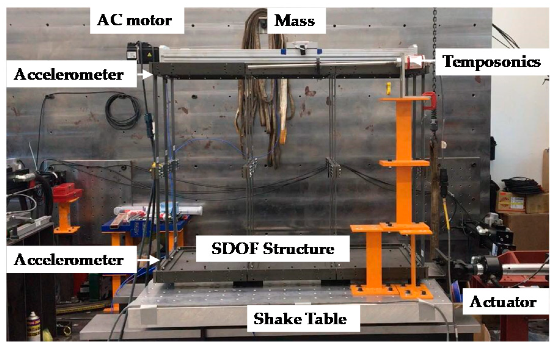
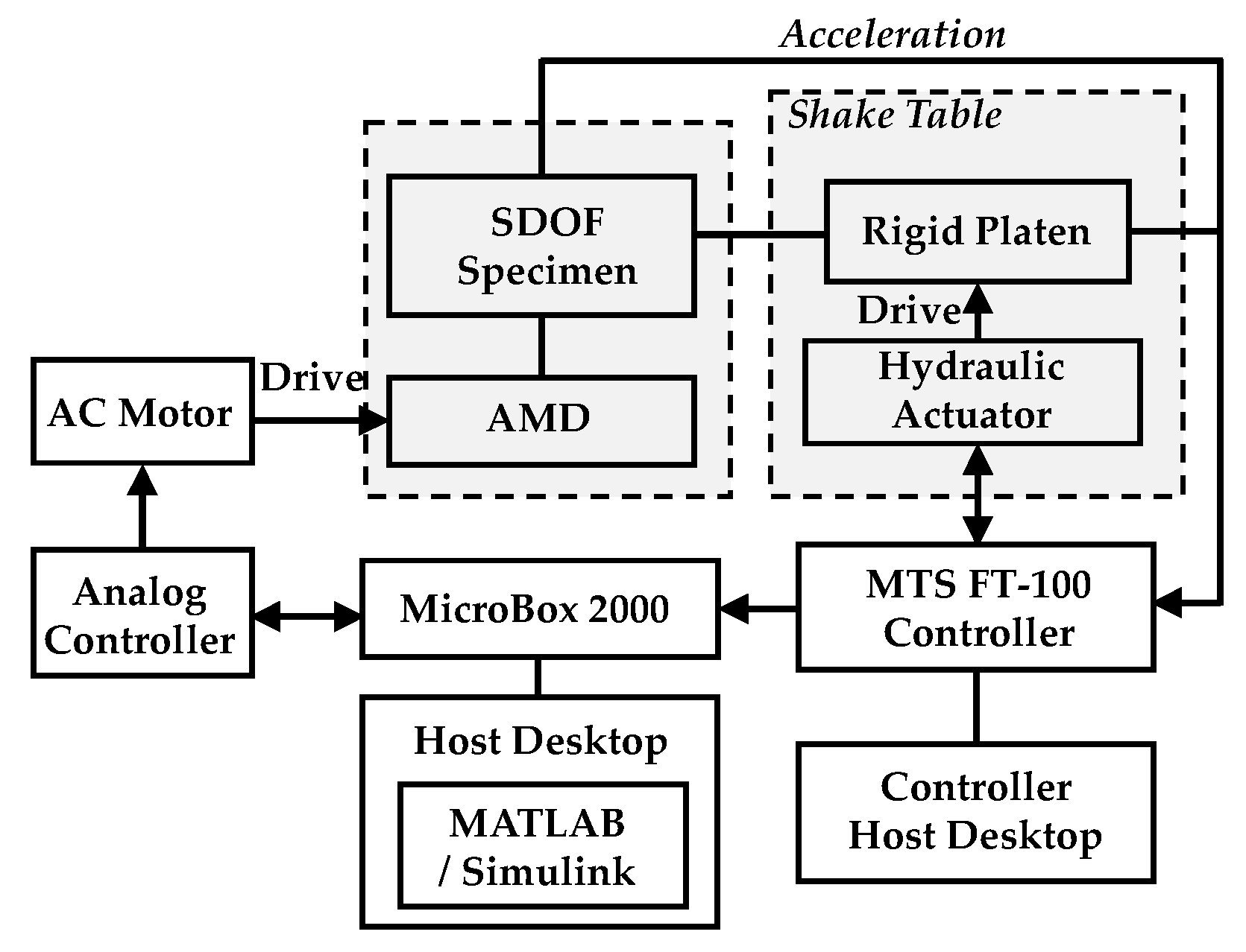
5.1. Experimental Setup

The machine learning based optimal control performance was evaluated by conducting shake table testing in the small-scale structural laboratory located in National Center for Research on Earthquake Engineering (NCREE) in Taipei, Taiwan [21]. Figure 11 shows the experimental setup. A single-degree-of-freedom (SDOF) shear building specimen made of aluminum alloy was designed and fabricated for experimental validation. The weight of the specimen was 450 N. The AMD installed on the top of specimen was composed of an AC motor, a guide screw, and a mass block. The weight of the mass block was 20 N, which was 4.4% weight of the specimen. The entire structural system was fixed on a rigid bottom plate, which was installed on the rigid platen of a shake table. The shake table was driven by a dynamic servo-hydraulic actuator with maximum stroke and force capacity of ±127 mm and ±15 kN, respectively. The dimension of the rigid platen made of aluminum was 1000 × 800 mm. An MTS FlexTest^® Controller FT-100 digital controller, manufactured by MTS Systems Corporation, Eden Prairie, MN, USA was used to control the actuator using a proportional-integral-derivative control algorithm. An analog controller converted voltage into current was used to control the torque of the motor. Three high-resolution MEMS accelerometers manufactured by Silicon Designs, Inc., Kirkland, WA, USA were installed on the bottom rigid plate connected to the shake table, the roof of specimen, and the mass block to measure the absolute acceleration. Each accelerometer was able to measure a range of acceleration of ±20 m/s². Note the control force of AMD was obtained by multiplying the mass of the mass block by the absolute acceleration measured from the accelerometer. Meanwhile, a Temposonics GH linear-position sensor, manufactured by MTS Systems Corporation, Eden Prairie, MN, USA was installed between the roof and the platen of shake table to measure the relative displacement of the specimen.

In order to implement the controller of AMD, a Micro-Box 2000 developed by TeraSoft Inc., Taipei, Taiwan was adopted which provided multi-function platform for rapid control prototyping applications. Three controllers were designed and implemented including the LQR-SOS, MLP-150, and ARX. The three controllers were built on the host desktop using MATLAB/Simulink and connected to I/O hardware with blocks provided by Simulink Real-Time. Executable C-code was compiled and downloaded onto the Micro-Box 2000 to run the control application. Meanwhile, the LQR-SOS required structural states for feedback control which were not measurable during the tests. As a result, a Kalman filter was essential to estimate the structural states for feedback control. In addition, the MLP and ARX took the measured acceleration as the input to calculate the control force. However, the acceleration measurement contained noise which could result in high-frequency control force and enlarge the acceleration response. Therefore, a 4th-order elliptic low-pass filter with a cutoff frequency of 15 Hz was designed. Both the Kalman filter and the low-pass filter were implemented using MATLAB/Simulink. The hardware and software layout for the experimental validation is depicted in Figure 12. The MATLAB/Simulink program was converted to C code and executed in Micro-Box 2000 which was running in real time. The shake table controlled by the MTS FT-100 controller excited the specimen. The seismic response of the specimen was measured and sent to the Micro-Box 2000 by the MTS FT-100 controller. Then the control force was calculated in real time and sent to the analog controller to drive the AMD. The mass block movement provided the inertial force which was equivalent to the achieved control force imposed on the specimen. The entire closed-loop control was repeated until the ground acceleration ended.

5.2. Experimental Results

System identification of the SDOF shear building specimen was conducted prior to designing the LQR for the AMD. The identified natural frequency and damping ratio of the specimen were 0.905 Hz and 0.25%, respectively. The SOS metaheuristic optimization approach was applied to minimize the objective function as exposed in Equation (12). Since the specimen had only single degree-of-freedom, the Equation (12) became to minimize the peak absolute acceleration of the specimen. The procedure of design of LQR as well as training of MLP and ARX models for the experiments are illustrated in Figure 13. During the optimization of weighting matrices using SOS, a BLWM with a PGA of 0.8 m/s², a bandwidth from 0 to 15 Hz, and a duration of 140 s was used to excite the identified structural model with a time step of 0.005 sec. Accordingly, the weightings Q and R in the cost function shown in Equation (6) were optimized and the optimal value of Q and R were 1.8357 and 100, respectively in the experimental validation. Accordingly, the state feedback gain K_g was obtained as [−0.2393, 0.1329]. Afterwards, the structural model was subjected to the band-limited white noise excitation again and the control force and structural acceleration were obtained. Then, MLP with 150 steps of acceleration (MLP-150) and the ARX controllers were trained offline using these data.

Eight of the fourteen earthquake ground acceleration records were selected as the excitation to the SDOF specimen. Note that the stroke of the AMD could limit the control force level applied to the specimen since the natural frequency of the specimen was 0.905 Hz. Therefore, the ground acceleration time histories were re-scaled to a PGA of 0.8 m/s² in the experimental validation. The LQR-SOS, MLP-150 and ARX were implemented in the experimental validation. A Kalman filter was designed based on the identified structural model in order to obtain the structural states for LQR state feedback control. Since both the MLP and ARX required the acceleration measured from the specimen to calculate the control force, the noise in the acceleration could result in high-frequency control force and enlarge the acceleration response. Therefore, a 4th-order elliptic low-pass filter with a cutoff frequency of 15 Hz was implemented for the measured acceleration.

Table 9. Seismic control performance of the experimental validating tests.

Controller	LQR-SOS			MLP-150			ARX
Earthquakes	J1/J2	J3	J4	J1/J2	J3	J4	J1/J2	J3	J4
El Centro	0.473	0.455	0.036	0.431	0.437	0.033	0.456	0.544	0.036
Chichi	0.668	0.690	0.021	0.672	0.752	0.026	0.693	0.728	0.027
Kobe	0.447	0.438	0.056	0.519	0.567	0.042	0.525	0.515	0.036
Northridge	0.899	0.885	0.030	0.776	0.841	0.032	0.843	0.832	0.038
Parkfield	0.449	0.414	0.039	0.389	0.446	0.036	0.441	0.501	0.031
Montenegro	0.671	0.641	0.043	0.613	0.616	0.035	0.635	0.642	0.034
Meinong	0.637	0.616	0.048	0.644	0.621	0.033	0.647	0.679	0.045
Capemendocino	0.743	0.685	0.041	0.764	0.839	0.051	0.790	0.787	0.041
Average	0.623	0.603	0.039	0.601	0.640	0.036	0.629	0.653	0.036

shows the experimental results of the three controllers with respect to the performance indices. Note that the specimen used in the validation was a SDOF shear building. Therefore, the performance indices J₁ and J₂ were identical. From Table 9, it is found the results of MLP-150 and ARX in the experimental validation are inferior to the numerical simulation results considering the effectiveness of LQR emulation. This is due to the fact that the structural states and acceleration were permanently accurate and precise in the numerical simulation, the error of the Kalman filter and effect of the low-pass filter could not be observed. Nevertheless, the overall performance of the trained MLP-150 and ARX models is considered fairly well comparing with the LQR-SOS. The performance indices of the three controllers in average are approximately within the same level. Figure 14 and Figure 15 illustrate the time histories of control force and structural response of the specimen, respectively when the specimen was subjected to El Centro earthquake. From Figure 14, it is investigated that there exists tracking error between the desired and achieved control force in the three control cases. The achieved control force is frequently smaller than the desired one. However, the tracking performance is considered acceptable considering the friction between the guide screw and the mass block. In addition, the control force time histories of the three control cases are similar in both frequency and magnitude. Similar trend can be also observed in the structural responses as depicted in Figure 15. It demonstrates that the MLP and ARX are able to emulate the LQR controller reasonably successful in the experimental validation.

6. Conclusions

Linear-quadratic regulator (LQR) has been widely applied to structural control as it minimizes a cost function formulated by weighted states and control inputs. However, LQR requires structural states for feedback control which may not be measurable in real application. Therefore, state estimation is indispensable which inevitably takes additional computation time and probably results in time delay during the control application. In addition, the control effectiveness is sensitive to the performance of the state estimator. If the estimated states are not accurate enough and robustly stable, the corresponding control performance become mediocre. In this study, machine learning technology has been applied to learn the behavior of an LQR with optimized weighting matrices such that the control force can be predicted directly from the measurements. Two neural network models have been applied for learning which include a multilayer perceptron (MLP) model and an autoregressive with exogenous inputs (ARX) model.

In the numerical simulation, the number of acceleration steps for training the MLP model is investigated. Simulation results indicate that 120, 150, and 200 acceleration steps led to stable and satisfactory simulation results. On the other hand, the ARX model takes the previous output as one of the inputs for training. Therefore, the number of inputs becomes much less than that required for the MLP model. Simulation results demonstrate that both MLP and ARX models predict the control force well in the control simulation model. Although the root-mean-square error of the ARX model is larger than that of the MLP model, the elapsed time for training the ARX model is significantly less than that for training the MPL model. As a result, the ARX model is suggested in real application. In the experimental validation, the control force time histories of the MLP and ARX models are close to that of the LQR in both frequency and magnitude. Similar results can be also observed with respect to the structural displacement and acceleration. It demonstrates that the MLP and ARX are able to emulate the LQR controller fairly well in real application. Conclusively, machine-learning based controllers can be well-trained to replace conventional state feedback controllers which generally require an observer or state estimator to obtain the states. Machine-learning based controllers simply collect the measurable response and calculate the corresponding control force similar to the control force generated from a conventional state feedback controller. Accordingly, the control performance of LQR has been successfully emulated and the effect of state estimation error on the seismic control performance of LQR has been reduced. Future works will be focused on inverse training strategy in order to calculate the control force directly from the relationship between the control device and the structural acceleration.

References

1. Saaed, T.E.; Nikolakopoulos, G.; Jonasson, J.E.; Hedlund, H. A state-of-the-art review of structural control systems. J. Sound Vib. 2015, 21, 919–937. [Google Scholar] [CrossRef]
2. Chang, C.C.; Yang, H.T.Y. Control of buildings using active tuned mass damper. J. Eng. Mech. 1995, 121, 355–366. [Google Scholar] [CrossRef]
3. Cao, H.; Reinhorn, A.M.; Soong, T.T. Design of active mass damper for a tall TV tower in Nanjing China. Eng. Struct. 1998, 20, 134–143. [Google Scholar] [CrossRef]
4. Dyke, S.J.; Spencer, B.F., Jr.; Quast, P.; Kaspari, D.C., Jr.; Sain, M.K. Implementation of an active mass driver using acceleration feedback control. Microcomput. Civ. Eng. 1996, 11, 305–323. [Google Scholar] [CrossRef]
5. Wu, J.C.; Yang, J.N. Active control of transmission tower under stochastic wind. J. Struct. Eng. 1998, 124, 1302–1312. [Google Scholar] [CrossRef]
6. Ghaboussi, J.; Joghataie, A. Active control of structures using neural networks. J. Eng. Mech. 1995, 121, 555–567. [Google Scholar] [CrossRef]
7. Rumelhart, D.E.; Hinton, G.E.; Williams, R.J. Learning representations by back-propagating errors. Nature 1986, 323, 533–536. [Google Scholar] [CrossRef]
8. Chen, H.M.; Tsai, K.H.; Qi, G.Z.; Yang, J.C.S. Neural network for structure control. J. Comput. Civ. Eng. 1995, 9, 168–176. [Google Scholar] [CrossRef]
9. Bani-Hani, K.; Ghaboussi, J. Nonlinear structural control using neural networks. J. Eng. Mech. 1998, 124, 319–327. [Google Scholar] [CrossRef]
10. Kim, J.T.; Jung, H.J.; Lee, I.W. Optimal structural control using neural networks. J. Eng. Mech. 2000, 126, 201–205. [Google Scholar] [CrossRef]
11. Hung, S.L.; Kao, C.Y.; Lee, J.C. Active pulse structural control using artificial neural networks. J. Eng. Mech. 2000, 126, 839–849. [Google Scholar] [CrossRef] [Green Version]
12. Cho, H.C.; Fadali, S.M.; Saiidi, M.S.; Lee, K.S. Neural network active control of structures with earthquake excitation. Int. J. Control Autom. Syst. 2005, 3, 202–210. [Google Scholar]
13. Lin, T.K.; Chang, K.C.; Chung, L.L.; Lin, Y.B. Active control with optical fiber sensors and neural networks. I: Theoretical analysis. J. Struct. Eng. 2006, 132, 1293–1303. [Google Scholar] [CrossRef]
14. Bani-Hani, K. Vibration control of wind-induced response of tall buildings with an active tuned mass damper using neural networks. Struct. Control Health Monit. 2007, 14, 83–108. [Google Scholar] [CrossRef]
15. Setio, H.D.; Gunawan, A.S. Numerical study of active mass damper application on cable-stayed bridge structure using artificial neural network algorithm. Int. J. Civ. Environ. Eng. 2017, 17, 1–17. [Google Scholar]
16. Chen, C.J.; Yang, S.M. Application neural network controller and active mass damper in structural vibration suppression. J. Intell. Fuzzy Syst. 2014, 27, 2835–2845. [Google Scholar] [CrossRef]
17. Cheng, M.Y.; Prayogo, D. Symbiotic organisms search: A new metaheuristic optimization algorithm. Comput. Struct. 2014, 139, 98–112. [Google Scholar] [CrossRef]
18. Amini, F.; Hazaveh, N.K.; Rad, A.A. Wavelet PSO-based LQR algorithm for optimal structural control using active tuned mass dampers. Comput.-Aided Civ. Infrastruct. Eng. 2013, 28, 542–557. [Google Scholar] [CrossRef]
19. Kingma, D.P.; Ba, J.L. Adam, A method for stochastic optimization. In Proceedings of the 3rd International Conference for Learning Representations, San Diego, CA, USA, 7–9 May 2015. [Google Scholar]
20. Jansen, L.M.; Dyke, S.J. Semiactive control strategies for MR dampers: Comparative study. J. Eng. Mech. 2000, 126, 795–803. [Google Scholar] [CrossRef] [Green Version]
21. Chen, P.C.; Ting, G.C.; Li, C.H. A versatile small-scale structural laboratory for novel experimental earthquake engineering. Earthq. Struct. 2020, 18, 337–348. [Google Scholar] [CrossRef]
Figure 1. Illustration of the mathematical model of a building with an active mass damper.
Applsci 10 05342 g001
Figure 2. Flowchart of symbiotic organism search.
Applsci 10 05342 g002
Figure 3. Blocked diagram of the training process. LQR: linear-quadratic regulator; ML: machine learning.
Applsci 10 05342 g003
Figure 4. Illustration of a multilayer perceptron model.
Applsci 10 05342 g004
Figure 5. Illustration of an autoregressive with exogenous inputs model.
Applsci 10 05342 g005
Figure 6. Illustration of the 10-story shear building with an active mass damper (AMD).
Applsci 10 05342 g006
Figure 7. Convergence curve of objective function using SOS (symbiotic organisms search).
Applsci 10 05342 g007
Figure 8. Control simulation model of the MLP (multilayer perceptron).
Applsci 10 05342 g008
Figure 9. Architectures of the exogenous inputs (ARX) neural network: (a) series-parallel, and (b) parallel.
Applsci 10 05342 g009
Figure 10. Control simulation model of the ARX (autoregressive with exogenous inputs).
Applsci 10 05342 g010
Figure 11. Experimental setup for the validating tests.
Applsci 10 05342 g011
Figure 12. Hardware and software layout for the validating tests.
Applsci 10 05342 g012
Figure 13. Flowchart of the design and training procedure for the experimental validation. BLWN: band-limited white noise.
Applsci 10 05342 g013
Figure 14. Time histories of the desired and achieved control force of the three controllers.
Applsci 10 05342 g014
Figure 15. Time histories of the structural responses in the experimental validation.
Applsci 10 05342 g015