Empirical Quasi-Static and Inverse Kinematics of Cable-Driven Parallel Manipulators Including Presence of Sagging


Abstract
1. Introduction
1.1. Motivation
1.2. Related Work
1.3. Contributions
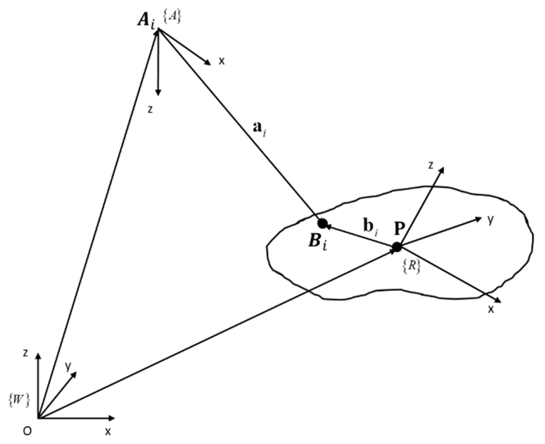
2. Cable-Driven Parallel Manipulators Model
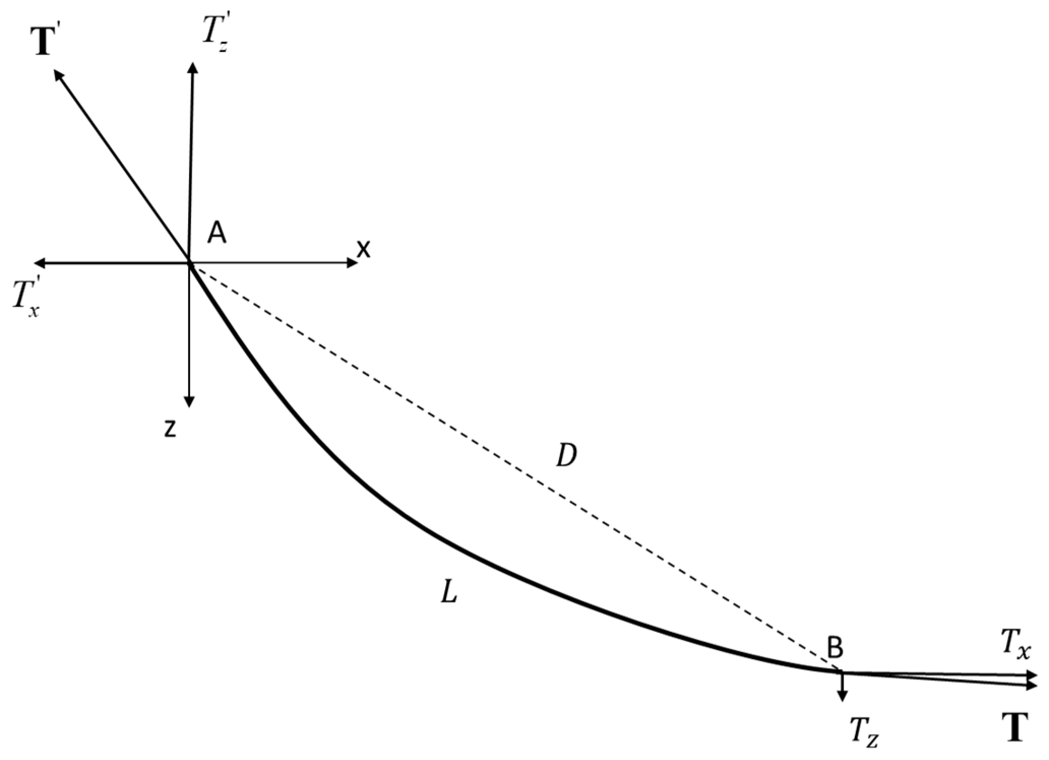
2.1. Sagging Cable Model
2.2. Quasi-Static and Inverse Kinematic Problem of Cable-Driven Parallel Manipulators
3. Quasi-Static and Inverse Kinematic Characteristics of Single Cable
4. Empirical Quasi-Static Model of Single cable
4.1. Analyze the Natural Limit of Tension Act on Free Extremity of Cable
4.2. Empirical Relationship between and
4.2.1. Relationship between and D
4.2.2. Relationship between and
4.3. Relationship between and
5. Relationship between Cable Unstrained Length and Cable Tension
5.1. Simplify the Problem
5.2. Relationship between and
5.2.1. Select Model
5.2.2. Relationship between and D
5.2.3. Relationship between and
5.2.4. Relationship between and
5.2.5. Relationship between L and
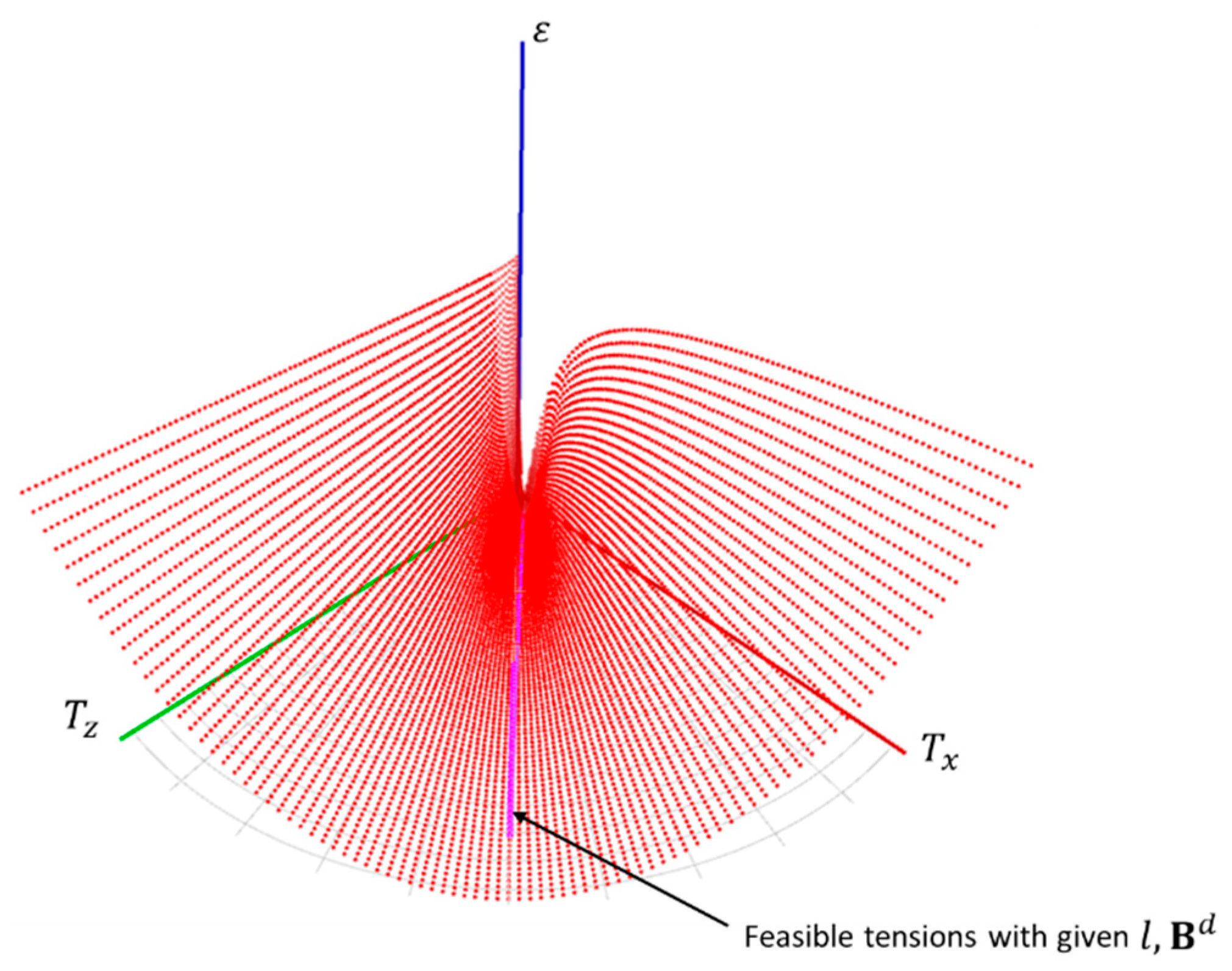
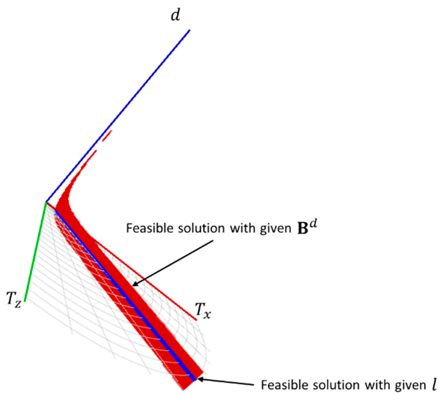
6. From Quasi-Statics to Inverse Kinematics of Cable-Driven Parallel Manipulators
7. Experiments and Results
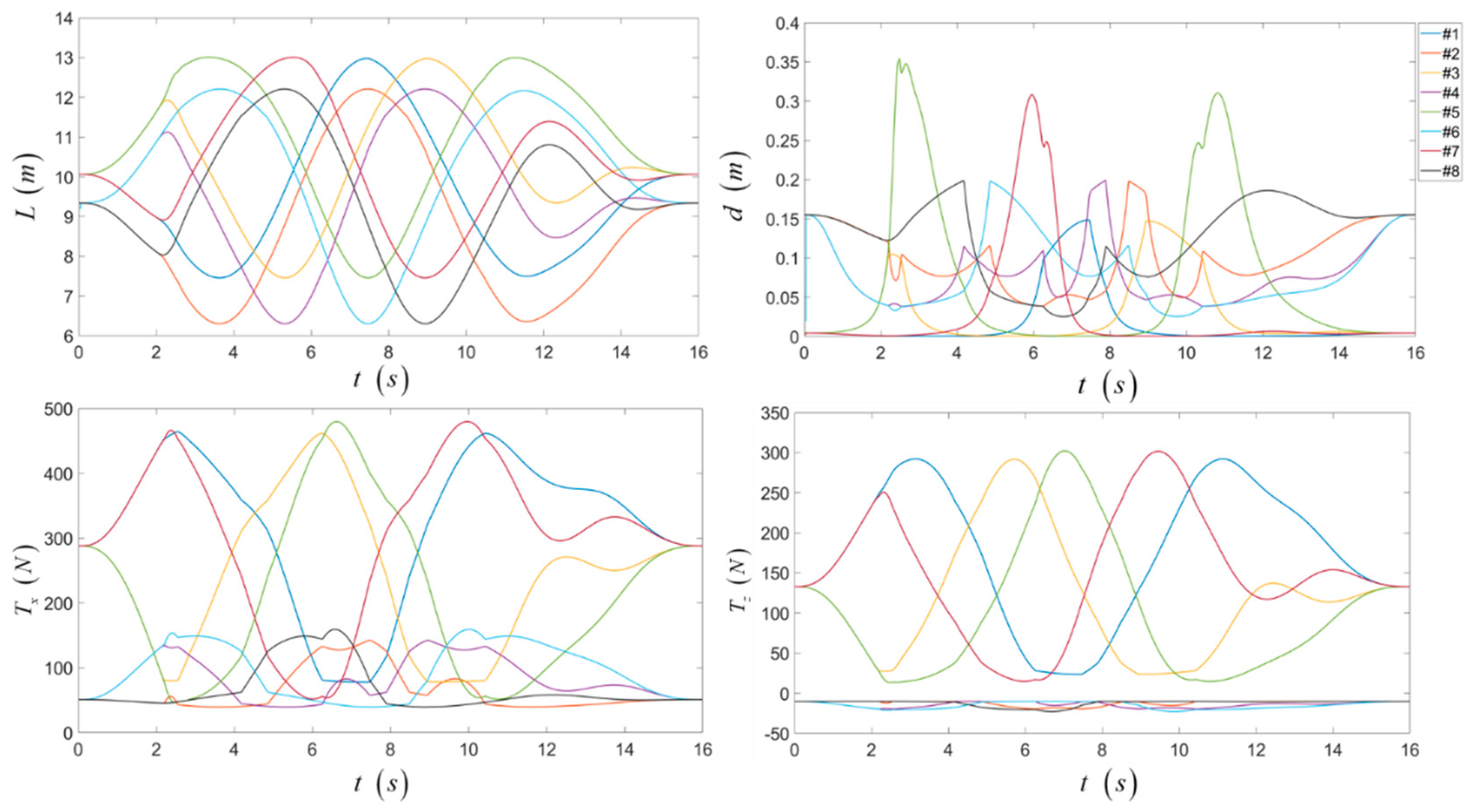
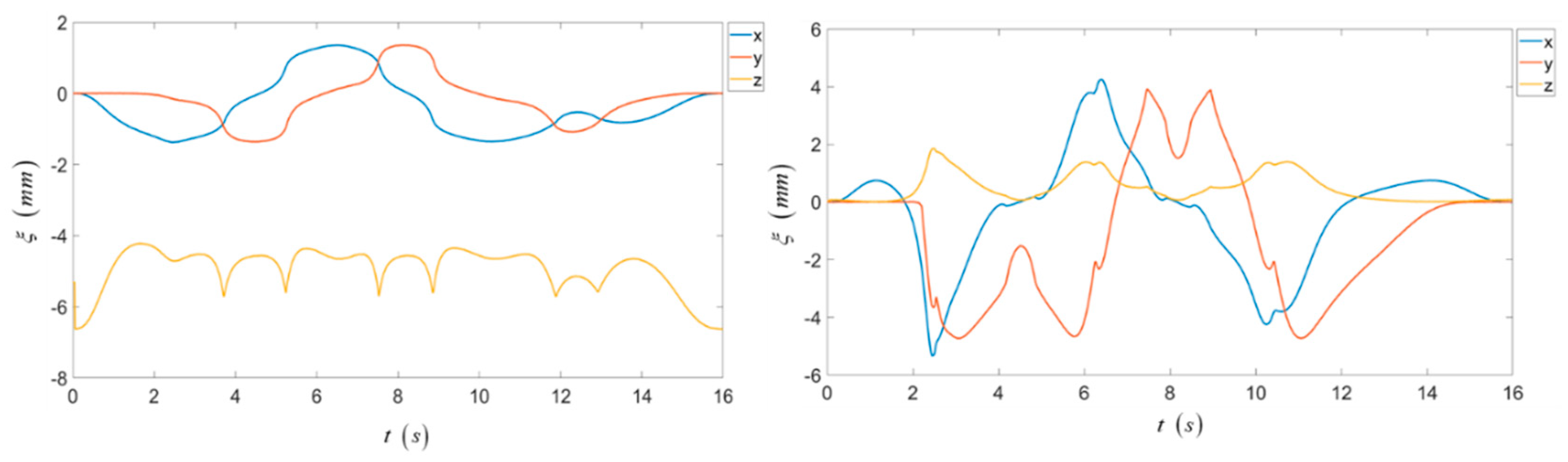
7.1. Simulation
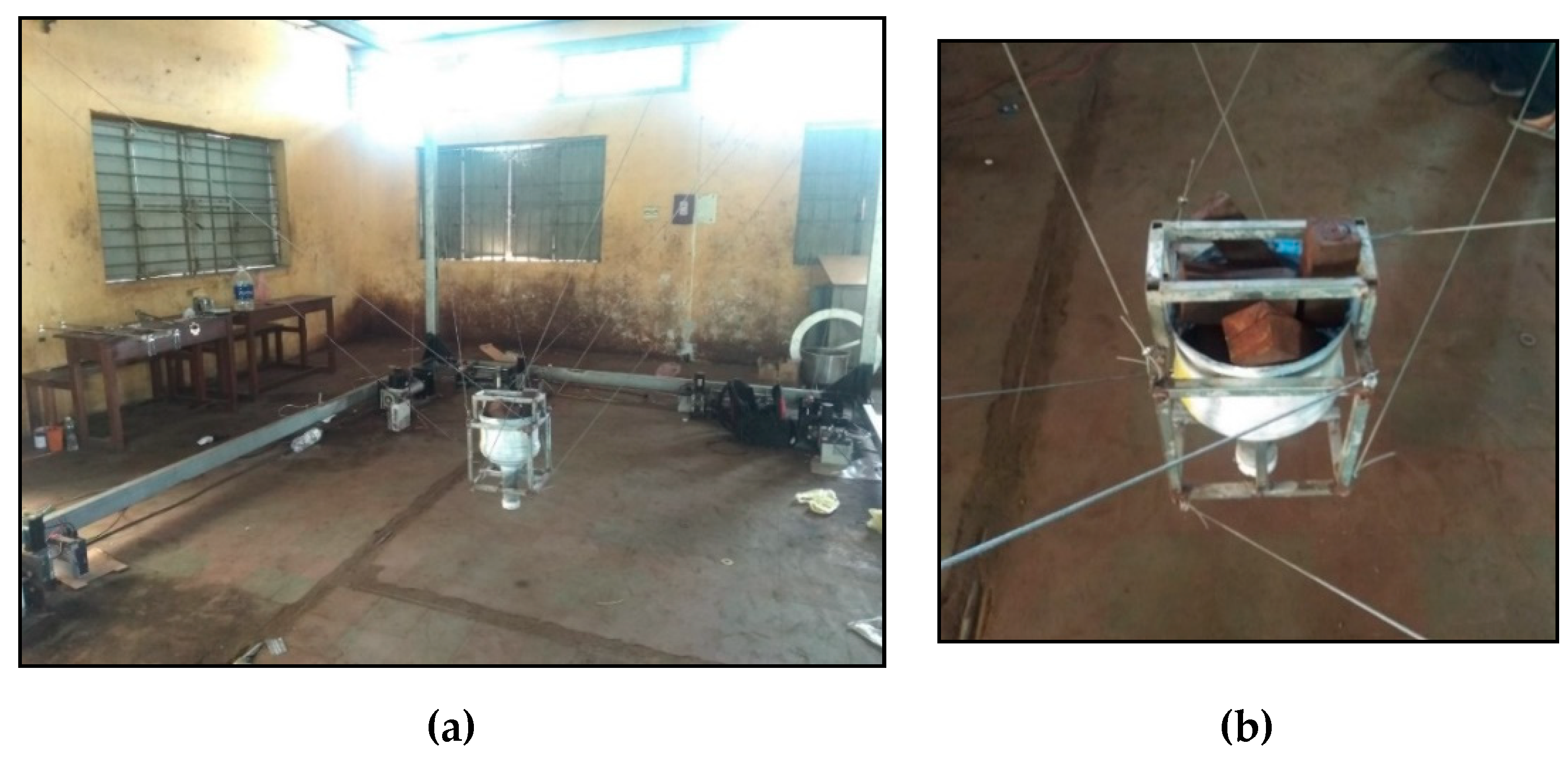
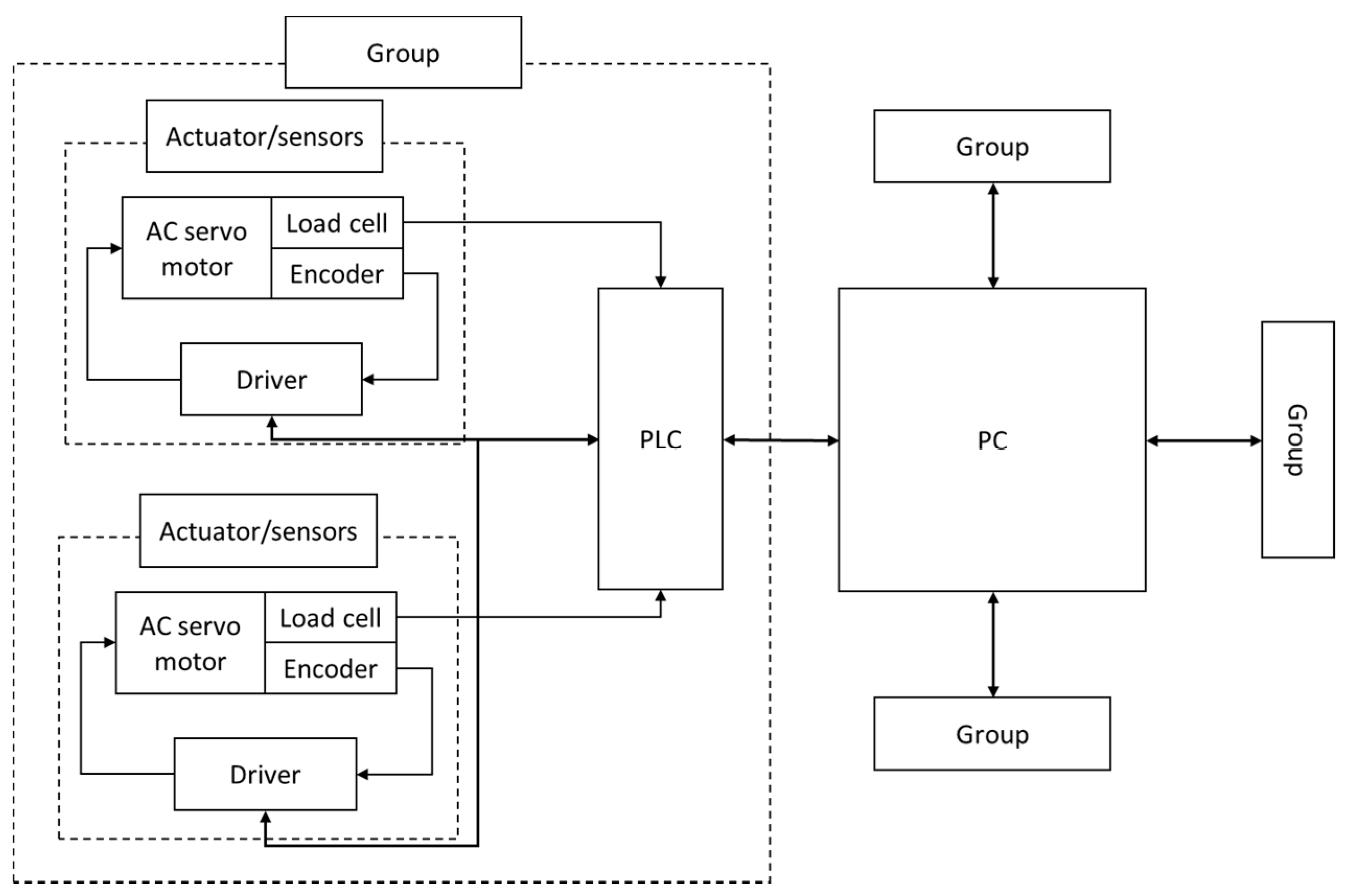
7.2. Experiment
8. Conclusions
- Analyzing and determining the boundaries of the wrench-feasible workspace in order to determine the set of all wrenches that CDPMs can apply without violating the boundaries of the tensions and load capacities of actuators;
- Due to the presence of unstrained cables and large inertia of the moving platform, the vibration is easily identifiable in CDPM. Vibration has a great impact on the dynamic behavior of the positioning accuracy and deviation on force distribution. Therefore, having a good analysis of vibration is a premise to developing a good dynamic model.
Author Contributions
Acknowledgments
Conflicts of Interest
References
- Vafaei, A.; Khosravi, M.A.; Taghirad, H.D. Modeling and control of cable driven parallel manipulators with elastic cables: Singular perturbation theory. In International Conference on Intelligent Robotics and Applications; Springer: Berlin/Heidelberg, Germany, 2011. [Google Scholar]
- Alias, C.; Nikolaev, I.; Magallanes, E.G.C.; Noche, B. An Overview of Warehousing Applications based on Cable Robot Technology in Logistics. In Proceedings of the 2018 IEEE International Conference on Service Operations and Logistics, and Informatics (SOLI), Singapore, 31 July–2 August 2018. [Google Scholar]
- Bosscher, P.; Williams, R.L., II; Bryson, L.S.; Castro-Lacouture, D. Cable-suspended robotic contour crafting system. Autom. Constr. 2007, 17, 45–55. [Google Scholar] [CrossRef]
- El-Ghazaly, G.; Gouttefarde, M.; Creuze, V. Adaptive terminal sliding mode control of a redundantly-actuated cable-driven parallel manipulator: CoGiRo. In Cable-Driven Parallel Robots; Springer: Cham, Switzerland, 2015; pp. 179–200. [Google Scholar]
- Oftadeh, R.; Aref, M.M.; Taghirad, H.D. Forward kinematic analysis of a planar cable driven redundant parallel manipulator using force sensors. In Proceedings of the 2010 IEEE/RSJ International Conference on Intelligent Robots and Systems, Taipei, Taiwan, 18–22 October 2010. [Google Scholar]
- Lamaury, J.; Gouttefarde, M.; Chemori, A.; Hervé, P.-E. Dual-space adaptive control of redundantly actuated cable-driven parallel robots. In Proceedings of the 2013 IEEE/RSJ International Conference on Intelligent Robots and Systems, Tokyo, Japan, 3–7 November 2013. [Google Scholar]
- Pott, A. An algorithm for real-time forward kinematics of cable-driven parallel robots. In Advances in Robot Kinematics: Motion in Man and Machine; Springer: Dordrecht, The Netherlands, 2010; pp. 529–538. [Google Scholar]
- Pott, A.; Schmidt, V. On the forward kinematics of cable-driven parallel robots. In Proceedings of the 2015 IEEE/RSJ International Conference on Intelligent Robots and Systems (IROS), Hamburg, Germany, 28 September–2 October 2015. [Google Scholar]
- Côté, A.F.; Cardou, P.; Gosselin, C. A tension distribution algorithm for cable-driven parallel robots operating beyond their wrench-feasible workspace. In Proceedings of the 2016 16th International Conference on Control, Automation and Systems (ICCAS), Gyeongju, Korea, 16–19 October 2016. [Google Scholar]
- Gouttefarde, M.; Lamaury, J.; Reichert, C.; Bruckmann, T. A versatile tension distribution algorithm for $ n $-DOF parallel robots driven by $ n+ 2$ cables. IEEE Trans. Robot. 2015, 31, 1444–1457. [Google Scholar] [CrossRef]
- Borgstrom, P.H.; Jordan, B.L.; Sukhatme, G.S.; Batalin, M.A.; Kaiser, W.J. Rapid computation of optimally safe tension distributions for parallel cable-driven robots. IEEE Trans. Robot. 2009, 25, 1271–1281. [Google Scholar] [CrossRef]
- Yuan, H.; Courteille, E.; Deblaise, D. Elastodynamic analysis of cable-driven parallel manipulators considering dynamic stiffness of sagging cables. In Proceedings of the 2014 IEEE International Conference on Robotics and Automation (ICRA), Hong Kong, China, 31 May–7 June 2014. [Google Scholar]
- Nguyen, D.Q.; Gouttefarde, M.; Company, O.; Pierrot, F. On the simplifications of cable model in static analysis of large-dimension cable-driven parallel robots. In Proceedings of the 2013 IEEE/RSJ International Conference on Intelligent Robots and Systems, Tokyo, Japan, 3–7 November 2013. [Google Scholar]
- Riehl, N.; Gouttefarde, M.; Krut, S.; Baradat, C.; Pierrot, F. Effects of non-negligible cable mass on the static behavior of large workspace cable-driven parallel mechanisms. In Proceedings of the 2009 IEEE International Conference on Robotics and Automation, Kobe, Japan, 12–17 May 2009. [Google Scholar]
- Merlet, J.-P.; Alexandre-dit-Sandretto, J. The forward kinematics of cable-driven parallel robots with sagging cables. In Cable-Driven Parallel Robots; Springer: Cham, Switzerland, 2015; pp. 3–15. [Google Scholar]
- Kozak, K.; Zhou, Q.; Wang, J. Static analysis of cable-driven manipulators with non-negligible cable mass. IEEE Trans. Robot. 2006, 22, 425–433. [Google Scholar] [CrossRef]
- Irvine, H.M. Cable Structures; The MIT Press: Cambridge, MA, USA, 1981; pp. 15–24. [Google Scholar]
- Merlet, J.-P. Some properties of the Irvine cable model and their use for the kinematic analysis of cable-driven parallel robots. Mech. Mach. Theory 2019, 135, 271–280. [Google Scholar] [CrossRef]
- Williams, R.L.; Gallina, P.; Rossi, A. Planar cable-direct-driven robots, part i: Kinematics and statics. In Proceedings of the 2001 ASME Design Technical Conference, 27th Design Automation Conference, Pittsburgh, PA, USA, 9–12 September 2001. [Google Scholar]
- Gouttefarde, M.; Collard, J.-F.; Riehl, N.; Baradat, C. Simplified static analysis of large-dimension parallel cable-driven robots. In Proceedings of the 2012 IEEE International Conference on Robotics and Automation, Saint Paul, MN, USA, 14–18 May 2012. [Google Scholar]
- Li, H.; Zhang, X.; Yao, R.; Sun, J.; Pan, G.; Zhu, W. Optimal force distribution based on slack rope model in the incompletely constrained cable-driven parallel mechanism of FAST telescope. In Cable-Driven Parallel Robots; Springer: Berlin/Heidelberg, Germany, 2013; pp. 87–102. [Google Scholar]
- Gouttefarde, M.; Collard, J.-F.; Riehl, N.; Baradat, C. Geometry selection of a redundantly actuated cable-suspended parallel robot. IEEE Trans. Robot. 2015, 31, 501–510. [Google Scholar] [CrossRef]
- Pott, A.; Mütherich, H.; Kraus, W.; Schmidt, V.; Miermeister, P.; Dietz, T.; Verl, A. IPAnema: A family of cable-driven parallel robots for industrial applications. In Cable-Driven Parallel Robots; Springer: Berlin/Heidelberg, Germany, 2013; pp. 119–134. [Google Scholar]


| Parameters | Experiment | Simulation |
|---|---|---|
| Fixed frame size | 3 m × 6 m × 3 m | 15 m × 11 m × 6 m |
| End-effector size | 0.3 m × 0.3 m × 0.5 m | 0.3 m × 0.3 m × 0.5 m |
| End-effector load | 50 kg | 50 kg |
| 0.09 kg/m | 0.067 kg/m | |
| 3.5 GPa | 2 GPa | |
| 4 mm2 | 2 mm2 |
| Desired Positions (m) | Actual Position (m) | Positioning Error (mm) |
|---|---|---|
| P1(0.22, −0.45, 1.43) | (0.2220, −0.4510, 1.4470) | 17.1464 |
| P2(−0.13, 1.42, 0.68) | (−0.1290, 1.4380, 0.7210) | 44.7884 |
| P3(−0.29, −0.25, 1.52) | (−0.2920, −0.2510, 1.5340) | 14.1774 |
| P4(0.30, 1.26, 2.31) | (0.3000, 1.2610, 2.3150) | 5.0990 |
| P5(−0.47, 0.80, 2.17) | (−0.4710, 0.8000, 2.1760) | 6.0828 |
| P6(0.48, −0.85, 0.72) | (0.4860, −0.8550, 0.7460) | 27.1477 |
| P7(−1.08, −0.75, 2.54) | (−1.0810, −0.7510, 2.5410) | 1.7321 |
| P8(0.26, 1.06, 0.44) | (0.2640, 1.0760, 0.4790) | 42.3438 |
| P9(0.45, −1.73, 1.71) | (0.4500, −1.7340, 1.7270) | 17.4642 |
| P10(0.67, 0.52, 2.02) | (0.6710, 0.5200, 2.0280) | 8.0623 |
© 2020 by the authors. Licensee MDPI, Basel, Switzerland. This article is an open access article distributed under the terms and conditions of the Creative Commons Attribution (CC BY) license (http://creativecommons.org/licenses/by/4.0/).
Share and Cite
Gia Luan, P.; Truong Thinh, N. Empirical Quasi-Static and Inverse Kinematics of Cable-Driven Parallel Manipulators Including Presence of Sagging. Appl. Sci. 2020, 10, 5318. https://doi.org/10.3390/app10155318
Gia Luan P, Truong Thinh N. Empirical Quasi-Static and Inverse Kinematics of Cable-Driven Parallel Manipulators Including Presence of Sagging. Applied Sciences. 2020; 10(15):5318. https://doi.org/10.3390/app10155318
Chicago/Turabian StyleGia Luan, Phan, and Nguyen Truong Thinh. 2020. "Empirical Quasi-Static and Inverse Kinematics of Cable-Driven Parallel Manipulators Including Presence of Sagging" Applied Sciences 10, no. 15: 5318. https://doi.org/10.3390/app10155318
APA StyleGia Luan, P., & Truong Thinh, N. (2020). Empirical Quasi-Static and Inverse Kinematics of Cable-Driven Parallel Manipulators Including Presence of Sagging. Applied Sciences, 10(15), 5318. https://doi.org/10.3390/app10155318