Numerical Simulation of Cavitation Erosion Aggressiveness Induced by Unsteady Cloud Cavitation

Abstract

A numerical investigation of the erosion aggressiveness of leading edge unsteady cloud cavitation based on the energy balance approach has been carried out to ascertain the main damaging mechanisms and the influence of the free stream flow velocity. A systematic approach has permitted the determination of the influence of several parameters on the spatial and temporal distribution of the erosion results comprising the selection of the cavitation model and the collapse driving pressure. In particular, the Zwart, Sauer and Kunz cavitation models have been compared as well as the use of instantaneous versus average pressure values. The numerical results have been compared against a series of experimental results obtained from pitting tests on copper and stainless steel specimens. Several cavitation erosion indicators have been defined and their accuracy to predict the experimental observations has been assessed and confirmed when using a material-dependent damaging threshold level. In summary, the use of the average pressure levels during a sufficient number of simulated shedding cycles combined with the Sauer cavitation model are the recommended parameters to achieve reliable results that reproduce the main erosion mechanisms found in cloud cavitation. Moreover, the proposed erosion indicators follow a power law as a function of the free stream flow velocity with exponents ranging from 3 to 5 depending on their definition.

1. Introduction

Cavitation is an unique phenomenon in the field of hydrodynamics that occurs when the local pressure in a liquid drops below a critical value, usually close to the vapor pressure, and results in the development of various types of vapor structures such as attached cavities, travelling bubbles, vortical cavities and bubble clouds [1]. Cavitation can typically take place in some widely-used hydraulic machines like pumps, turbines and naval propellers. As a matter of fact, cavitation is often associated with some unwanted consequences like machine performance deterioration, cavitation noise, cavitation-induced vibration and cavitation erosion of solid surfaces [2].

Among the problems caused by cavitation, erosion is the one of the most complex ones since it involves the interaction between fluids and structures. Actually, cavitation erosion is caused by the collapse of the cavities. It has been observed that the collapse of a bubble is a condensation process that ends with the compression of the vapor and the subsequent emission of a shock wave creating a pressure pulse with a very strong amplitude. If the collapse takes place close to a solid wall, a high-speed liquid microjet forms, crosses the bubble and impacts the wall resulting in a very high impulsive pressure. If the impulsive forces resulting either from the impact of the microjet or the shockwave exceed the material threshold, such as its yield stress or its ultimate strength, local damage will be induced [1].

Advanced cavitation erosion may cause severe damage to components of hydraulic machines causing higher maintenance costs and deterioration of machine performance together with aggravated vibrations and noise. For example, turbine runners, fluid bearings and pump impellers among others may need replacement after several weeks/months of operation or require regular repair [2]. Therefore, from an industrial point of view concerning both design and maintenance, the evaluation of the erosive power of cavitating flows and the prediction of the material damage remains a major concern to manufacturers and operators. In this sense, several methodologies have been developed to predict cavitation erosion using Computational Fluid Dynamics (CFD) and Structural Mechanics.

A first approach focuses on the Fluid–Structure Interaction (FSI) between the cavitation phenomenon and the response of the solid boundary. Hsiao et al., [3] developed an in-house code based on FSI to study the material deformation due to the impact pressure caused by the collapse of a single bubble under different configurations, which provides a good resolution between flow field and material surface. Fivel et al., [4,5,6] proposed a one-way simulation method to compute the cavitation erosion based on the histogram of repetitive impact loads obtained experimentally from pitting tests and the analysis of the response of the material to them. However, the authors acknowledged that this approach to predict cavitation erosion needed further development. In addition, Joshi et al., [7,8] investigated the effect of some bubble and material properties (e.g., stand-off ratio, bubble size, driving pressure, strain rate, etc.) on the induced cavitation erosion by employing a meshless Smooth Particle Hydrodynamic (SPH) solver. More specifically, they found that the stand-off ratio has a significant effect on the erosion that permits to explain that an attached cavity has more potential to accelerate the initial damage, i.e., it requires a smaller incubation time, whereas a detached cavity leads to a higher erosion rate. Moreover, they pointed out that the strain rate effect should not be neglected in the constitutive model of the solid and that the peak pressure on the solid does not coincide with the region of maximum erosion. In summary, the SPH modelling approach represents an accurate theoretical background and, therefore, it allows exploring the FSI mechanism of cavitation erosion and stablishing the relationship between the erosion intensity and the material properties. Nonetheless, its practical application to predict the erosion in hydraulic machinery is still limited since cavitation can take different patterns and the erosion is mainly caused by large-scale unsteady cavitation forms.

A second approach consists of using the Eulerian–Lagrangian method, which treats the macroscopic flow field using Eulerian mechanics and the individual microscopic bubbles using Lagrangian mechanics. Ochiai et al. [9] obtained the macroscopic flow field by solving the continuity, momentum and energy equations of a compressible two-phase flow. For the simulation of the microscopic bubbles, they considered that they follow the equation of motion driven by the pressure gradient, the drag and the virtual mass force, and they used the equation of bubble oscillation to evaluate the evolution of bubble radius. Finally, the cavitation erosion characteristics were predicted using the impact pressures on the wall surface induced by the propagating pressure waves induced by the bubble collapses. Similarly, Wang and Zhu [10] applied Large Eddy Simulation (LES) to obtain the unsteady ambient pressures and velocity profiles around the bubbles and employed the Rayleigh–Plesset equation to determine the bubble radius. They predicted the cavitation erosion following the evolution of several representative bubbles in the averaged unsteady flow with cavitation. Although this method has the best theoretical background as it considers the bubble rebounds during the collapse and the macroscopic flow, it is uninfluenced by the bubble dynamics. Another problem lies in the choice of the bubbles’ injection points because they play a major role in the predicted erosion intensity [11].

The third approach, developed by Schmidt et al., [12,13], consists of predicting the impact load spectra of a cavitating flow. This method, considers the two-phase flow as homogeneous, compressible and inviscid, and it resolves the collapse-induced pressure waves to determine the spectrum of collapse events in the fluid domain. Blume and Skoda [14] used this method to assess the erosive cavitation flow around a hydrofoil with circular leading edge and obtained a good agreement with the experimental results. However, they indicated that this approach requires a very fine computational mesh in order to capture all scales of cavitation events. Moreover, a very short time step was required because shock waves, which propagate at the speed of sound in water, needed to be resolved near the solid wall. Consequently, the practical implementation of this method is very limited. For instance, this would require a very high computational cost and take too much time to simulate any full scale components, e.g., marine propellers.

The last approach, which is the most widely applied one, only resolves the macroscopic cavitating flow field and predicts the cavitation aggressiveness by using different erosion models based on the flow properties. For example, Nohmi et al., [15] developed four erosion indices which were based on pressure and volume fraction time derivatives as well as on absolute pressure differences. Li et al., [16] stated a numerical erosion model where the rapid increase of the local static pressure needed to exceed a certain threshold level for erosion to occur. Fortes-Patella et al., [17,18] suggested an energy balance approach where the potential energy of the macroscopic cavitation structures was regarded as the main factor that generates erosion. Thus, the potential energy of a cavitation cloud is supposed to be converted into acoustic energy in the form of pressure waves. These pressure waves travel through the fluid and are able to damage the solid wall. Koukouvinis et al., [19] defined a Cavitation Aggressiveness Index (CAI) based on the total derivative of pressure on the surface with values from zero that indicates the level of the hydrodynamic cavitation aggressiveness. Lloyd’s Register Technical Investigation Department [20] applied Detached Eddy Simulation (DES) to simulate the cavitating flow and obtained good predictions of the eroded regions based on its own functions, but few details about them can be found in the open literature. Unlike the above mentioned erosion models in which the pressure wave is considered to be responsible for the cavitation erosion, some researchers assumed that the high-speed microjet was the main mechanism provoking the cavitation erosion. Dular et al., [21] proposed an erosion model where the velocity of the microjet needed to exceed a certain threshold to be erosive for a given material. Following this work, Peters et al. [22] calculated the erosion potential of a cavitating flow based the accumulation of the dimensionless intensity coefficient, defined by the ratio of the jet velocity to a threshold velocity value, on every element face along the total calculation time. The advantage of these approaches is that there are no critical requirements regarding the cell size and the time step and consequently the calculation time becomes more reasonable than for instance the methods included in the third approach. Nevertheless, they need to be further validated with experiments because they involve the use of some empirical coefficients.

Among the erosion models discussed above, the model proposed by Fortes-Patella et al. [17,18] has been widely used because it has been validated by various researchers and it provides a good agreement with the experiments [23,24,25,26,27]. Another reason for its popularity is that it has also been applied to industrial and engineering cases such as marine propellers [25] and pumps [28]. In spite of that, some uncertainties still need to be investigated and discussed to improve its performance and applicability. Therefore, the present work has been devoted to simulate systematically the erosion induced by unsteady cloud cavitation on the surface of a 2D hydrofoil and to investigate the factors influencing the erosion results including the selection of the cavitation model and of the driving pressure in the erosion model. Moreover, the main mechanisms of cavitation erosion have also been discussed by comparing the numerical results with the experimental observations. Finally, the influence of the free stream velocity and the dynamic behavior of the cavitation on the estimated erosion power has also been estimated based on the collapse efficiency.

2. Experiment Description and Numerical Model

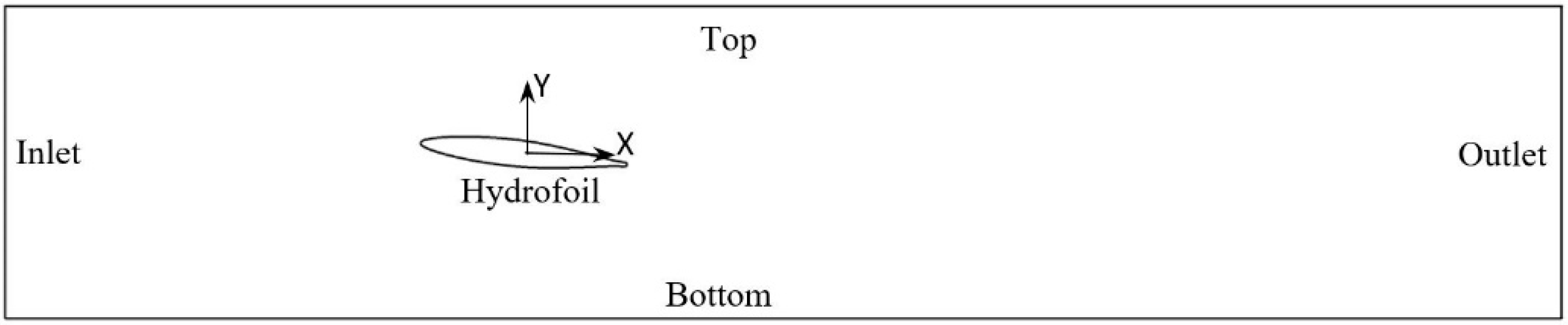
2.1. Experiment Description

The experimental conditions and results used to validate the numerical models are listed in

Table 1. Flow conditions and results for the validation experiment [29].

α [°]	l/c [–]	Uinf [m/s]	σ [-]	f [Hz]	St [-]
6	40	15	1.55	96.1	0.26
6	40	20	1.58	132.8	0.27
6	40	25	1.60	175.5	0.28
6	40	30	1.62	225.8	0.30

, comprising the hydrofoil incidence angle, a, the chord length, c, the free stream velocity, U_inf, the cavity length, l, the cavitation number, σ, the shedding frequency, f, and the Strouhal number, St. σ and St have been calculated with Equations (1) and (2), respectively, where P_in and P_v are the inlet and the vapor saturation pressures, respectively. The computational fluid domain corresponding to the cavitation tunnel test section is shown in Figure 1 and a more detailed description of experiment can be found in Escaler et al. [29] and Couty [30].

$$\sigma =\frac{P_{in}-P_v}{0.5{\rho }_l{U}_{\inf }{}^2}$$

(1)

$$St=\frac{fl}{U_{\inf }}$$

(2)

In the experiment, material specimens 30 mm in width made of standard copper and stainless steel polished down to mirror were mounted along the hydrofoil suction side at different chord positions. The specimens were obtained by an accurate electroerosion machining, glued with cyanoacrylate adhesive and removed after the tests by heating to 400 °C. The erosion intensity was assessed with a statistical analysis of the pitting data measured on the specimens during the incubating period. The pitting results were quantified with the mean pitting rate at the specimen location k, τ_n (k), and the mean volume deformation rate at location k, τ_v (k), which were respectively defined as:

$${\tau }_n\left(k\right)=\frac{N_k}{T_{pit}\times L_x\times L_y}$$

(3)

$${\tau }_v\left(k\right)=\frac{{\displaystyle \sum Vd\left(x_i,y_i\right)}}{T_{pit}\times L_x\times L_y}$$

(4)

where N_k is the number of cavitation impacts on location k, L_x and L_y are the side lengths of the tested specimen and T_pit is the time duration of the pitting test. Vd (x_i, y_i) represents the volume of the indentations on the surface at position (x_i, y_i), which was measured with a 3D profilometer.

Figure 2 presents the cavitation erosion results obtained for a U_inf of 20 m/s for two different materials: copper and stainless steel. Firstly, the influence of the material strength can be seen by comparing the amplitudes of the erosion indicators for copper in Figure 2a with those for stainless steel in Figure 2b. For copper, the maximum values of τ_n(k) are of about 0.03 mm^–2s⁻¹ at 40% of the chord and the maximum values of τ_v(k) are of about 160 μm³mm⁻²s⁻¹ at 50% of the chord. Meanwhile, the maximum τ_n(k) and τ_v(k) values are of about 0.0004 mm⁻²s⁻¹ and 1.9 μm³mm⁻²s⁻¹, respectively, at 50% of the chord for stainless steel. Therefore, the pitting rate suffered by the copper is almost two orders of magnitude higher than that for stainless steel. Regarding the location of the damages, the most eroded areas for both materials are found approximately in the range from 40 to 50% of the chord, as expected, because they have been submitted to the same cavitation conditions and the cavity closure region was located at 40% of the chord (l/c = 0.4) as indicated in Table 1. For copper, τ_n(k) shows the maximum at 40% of the chord but τ_v(k) shows the maximum at 50% of the chord. This seems to indicate that the hydrofoil surface suffers a large amount of impacts with small intensity at 40% and a lower number of impacts with a stronger intensity at 50%. A slightly different erosion pattern is found for stainless steel since it presents the maximum τ_n(k) in the range from 40% to 50% but the τ_v(k) shows a minimum value at 40% and a maximum value only at 50%. Likewise, the pitting results under other operating conditions show a similar trend as for this condition. Therefore, the erosion results presented on Figure 2 will be used as the reference to validate the numerical predictions.

2.2. Numerical Model

The homogeneous mixture assumption has been used to model the two-phase flow. Thus, velocity and pressures are shared by water and vapor phases and the governing Navier–Stokes equations for the mixture are:

$$\frac{\partial {\rho }_m}{\partial t}+\frac{\partial }{\partial x_i}\left({\rho }_m{u}_i\right)=0$$

(5)

$$\frac{\partial }{\partial t}({\rho }_m{u}_i)+\frac{\partial }{\partial x_j}({\rho }_m{u}_i{u}_j)=-\frac{\partial p}{\partial x_i}+\frac{\partial }{\partial x_j}\left[{\mu }_m\left(\frac{\partial u_i}{\partial x_j}+\frac{\partial u_j}{\partial x_i}-\frac{2}{3}{\delta }_{ij}\frac{\partial u_k}{\partial x_k}\right)\right]$$

(6)

where u is the velocity, p is the pressure, t is the time, μ_m is the mixture dynamic viscosity defined by μ_m = μ_vα_v + μ_l(1 − α_v) and ρ_m is mixture density calculated by ρ_m = ρ_vα_v + ρ_l(1 − α_v).

In the present simulation, the Reynolds Averaged Navier–Stokes (RANS) approach was used, in which the instantaneous quantities are decomposed into the mean and the fluctuating components, i.e., the instantaneous velocity u_i is equal to:

$$u_i=\overline{u_i}+u_i{}^{\prime }$$

(7)

Using Equation (7) to replace the instantaneous quantities of all the variables in Equations (5) and (6), the RANS equations are obtained:

$$\frac{\partial \overline{{\rho }_m}}{\partial t}+\frac{\partial }{\partial x_i}\left(\overline{{\rho }_m}\overline{u_i}\right)=0$$

(8)

$$\frac{\partial }{\partial t}(\overline{{\rho }_m}\overline{u_i})+\frac{\partial }{\partial x_j}(\overline{{\rho }_m}\overline{u_i}\overline{u_j})=-\frac{\partial \overline{p}}{\partial x_i}+\frac{\partial }{\partial x_j}\left[{\mu }_m\left(\frac{\partial \overline{u_i}}{\partial x_j}+\frac{\partial \overline{u_j}}{\partial x_i}-\frac{2}{3}{\delta }_{ij}\frac{\partial \overline{u_k}}{\partial x_k}\right)\right]+\frac{\partial }{\partial x_j}\left(-\overline{{\rho }_m}\overline{u_i{}^{\prime }{u}_j{}^{\prime }}\right)$$

(9)

Equations (8) and (9) have the same general form as the instantaneous Navier–Stokes equations, with the velocities and other solution variables now representing time-averaged values, and a series of new additional terms such as, $\rho \overline{u_i^{\prime }{u_j}^{\prime }}$, which are known as the Reynolds stresses induced by the turbulence. In order to close this system of equations, there are two approaches: the first one is based on the eddy-viscosity hypothesis, which relates the Reynolds stresses to the mean flow; the second one is based on solving the transport equation for all the components of the Reynolds stress tensor. In our case, the former method has been used, so a turbulent eddy viscosity, μ_t, has been introduced to model the effect of the Reynolds stresses, and the final momentum equation to be solved becomes:

$$\frac{\partial }{\partial t}(\overline{{\rho }_m}\overline{u_i})+\frac{\partial }{\partial x_j}(\overline{{\rho }_m}\overline{u_i}\overline{u_j})=-\frac{\partial \overline{p}}{\partial x_i}+\frac{\partial }{\partial x_j}\left[\left({\mu }_m+{\mu }_t\right)\left(\frac{\partial \overline{u_i}}{\partial x_j}+\frac{\partial \overline{u_j}}{\partial x_i}-\frac{2}{3}{\delta }_{ij}\frac{\partial \overline{u_k}}{\partial x_k}\right)\right]$$

(10)

In addition, a vapor volume fraction transport equation (Equation (11)) is used to consider the mass transfer between vapor and water:

$$\frac{\partial {\alpha }_v}{\partial t}+\nabla \cdot \left({\alpha }_{v}u\right)=\frac{\dot{m}}{{\rho }_v}$$

(11)

where the term $\dot{m}$ represents the mass transfer rate between the two phases.

For the current simulation, the turbulent viscosity, μ_t, in Equation (10) has been calculated with the SST k-ω model according our previous investigation [31], and μ_t has been defined as:

$${\mu }_t=\frac{f(\rho )a_1{k}^2}{\max (a_1\omega ,S{F}_2)}$$

(12)

where a₁ = 0.31, F₂ is a blending function which restricts the limiter to the wall boundary layer, S is an invariant measure of the strain rate and k and ω are the turbulence kinetic energy and frequency, respectively. In addition, f(ρ) is the density correction to reduce the over-predicted turbulent viscosity as proposed by Reboud et al. [32]:

$$f(\rho )={\rho }_v+{\left(1-{\alpha }_v\right)}^n({\rho }_l-{\rho }_v)$$

(13)

where n is the exponential coefficient which should be specified with a value of 10.

Besides, the effects of the cavitation models developed by Zwart [33], Sauer [34] and Kunz [35] on the prediction of erosion were investigated.

Table 2. Mathematical expressions of the cavitation models.

Model	$\dot{\mathit{m}}$ (P < Pv)	$\dot{\mathit{m}}$ (P > Pv)
Zwart	$C_{prod}\frac{3{\alpha }_{nuc}(1-{\alpha }_v){\rho }_v}{R_B}\sqrt{\frac{2}{3}\frac{\left(p_v-p\right)}{{\rho }_l}}$	$-C_{dest}\frac{3{\alpha }_v{\rho }_v}{R_B}\sqrt{\frac{2}{3}\frac{\left(p-p_v\right)}{{\rho }_l}}$
Sauer	$\frac{{\rho }_v{\rho }_l}{\rho }{\alpha }_v(1-{\alpha }_v)\frac{3}{R_B}\sqrt{\frac{2}{3}\frac{\left(p_v-p\right)}{{\rho }_l}}$	$-\frac{{\rho }_v{\rho }_l}{\rho }{\alpha }_v(1-{\alpha }_v)\frac{3}{R_B}\sqrt{\frac{2}{3}\frac{\left(p-p_v\right)}{{\rho }_l}}$
Kunz	$\frac{C_{dest}{\rho }_v{\alpha }_v{(1-{\alpha }_v)}^2}{t_{\infty }}+\frac{C_{prod}{\rho }_v(1-{\alpha }_v)\min \left[0,p-p_v\right]}{(0.5{\rho }_l{U}_{\inf }^2)t_{\infty }}$	$-\frac{C_{dest}{\rho }_v{\alpha }_v{(1-{\alpha }_v)}^2}{t_{\infty }}$

lists the mathematical equations describing each of these cavitation models where R_B in the Zwart model is the vapor bubble radius with a constant value of 10^-6 m. Meanwhile, in the Sauer model, it is a variable value that is function of the local vapor volume fraction. α_nuc is the nucleation site volume fraction with a default value of 0.0005. Then, t_∞ = C/U_inf is the mean time scale and C_prod and C_dest are the empirical coefficients for vaporization and condensation, respectively, which were taken as 50 and 0.01 for the Zwart model, and 100 and 100 for the Kunz model.

The solution strategy adopted for the current simulations was based on our previous work [31] where the influence of the numerical setting was investigated in detail. Consequently, a medium-sized mesh of 29,749 elements with y+ values in the boundary layers ranging from 0.1 to 3 with a mean value of 1.2 was used. A time step of 3⋅10⁻⁵ s corresponding to a Root Mean Square (RMS) Courant number of 1.6 was set as well as several successive iterations within each physical time step. A very small residual criterion of 10⁻⁸ and a large iterative number were set to march the solution towards convergence in every time step. The pressure-velocity direct coupling method was used to solve the governing equations. The high-resolution scheme was used for the convection terms. The second-order implicit time scheme was used for the transient term. To accelerate convergence, a series of transient simulations were run from previous steady state models. The simulations were carried out in parallel using twelve cores of an Intel^®Core™ i7-8700 K CPU equipped with 32 GB of RAM. Every unsteady simulation was stopped after at least ten cavity shedding cycles were captured, which took around 12 h for each case. In addition, much effort was taken on building the relationship between the cavity structures and their corresponding erosion intensities during the postprocessing of the obtained results. To achieve a very precise prediction of the position of cavity closure region, which is needed to simulate cavitation erosion [24,36], the cavitation number had to be adjusted to match exactly the same cavity length than in the experiment. Therefore, a cavitation number of 1.55 was used in the simulation, which was based on cavitation tunnel inlet pressure, as compared to the cavitation number of 1.58 set in the experiment.

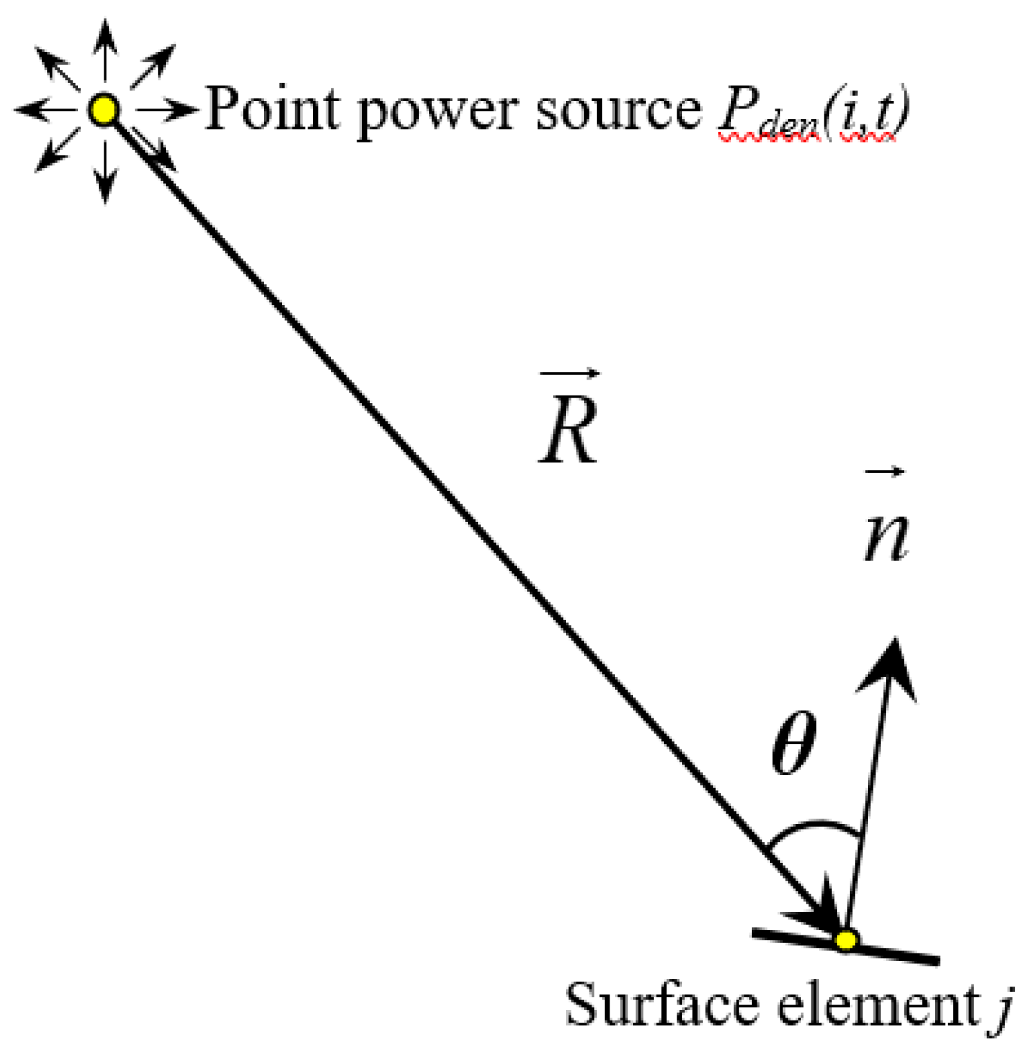
2.3. Cavitation Erosion Model

The cavitation erosion model used in the calculations was developed by Fortes-Patella et al. [17,18]. In this model, the pressure waves emitted during the cavitation collapses that reach the solid wall are the main mechanism responsible for erosion damage. The potential energy of a vapor structure in the fluid domain is defined as:

$$E_{pot}=\Delta p{V}_{vap}=(p_d-p_{vap})V_{vap}$$

(14)

where V_vap is the volume of the vapor structure and p_d is the driving pressure which forces its collapse. Then an instantaneous potential power, P_pot, can be defined with Lagrangian time derivatives as expressed with Equation (15):

$$P_{pot}=\frac{D{E}_{pot}}{Dt}=(p_d-p_{vap})\frac{D{V}_{vap}}{Dt}+\frac{Dp}{Dt}{V}_{vap}$$

(15)

Because the vapor volume is related to the vapor volume fraction, α_v = V_vap/V_cell, the potential power in each cell or the potential power density, P_den, can be written as:

$$P_{den}=\frac{P_{pot}}{V_{\mathrm{cell}}}=(p_d-p_{vap})\frac{D{\alpha }_v}{Dt}+\frac{Dp}{Dt}{\alpha }_v$$

(16)

Leclerc et al., [36] found that the second term on the right-hand side of Equation (16) is negligible compared to the first term and they assumed that P_pot is released instantaneously only when condensation takes place. This implies that only the first term on the right-hand side of Equation (16) contributes to the radiated power and only if the time derivative of α_v is positive. Therefore, P_den can be simplified to Equation (17):

$$P_{den}=\frac{p_{pot}}{V_{cell}}=(p_d-p_{vap})\frac{D{\alpha }_v}{Dt}$$

(17)

Note that P_pot is defined with Lagrangian time derivatives, which can be obtained substituting the sum of the first and second terms in the right-hand side of Equation (11) with the following relation:

$$\frac{D{\alpha }_v}{Dt}=\frac{\partial {\alpha }_v}{\partial t}+\nabla \cdot ({\alpha }_{v}u)-{\alpha }_v\nabla \cdot u$$

(18)

Besides, the divergence term, $\nabla \cdot \mathrm{u}$, is actually another form of continuity equation (Equation (5)) defined as ∇ $\cdot u=\dot{m}\left(\frac{1}{{\rho }_v}-\frac{1}{{\rho }_l}\right)$ [26]. Hence, Equation (18) can be rewritten as:

$$\frac{D{\alpha }_v}{Dt}=\frac{\dot{m}}{{\rho }_v}-{\alpha }_v\dot{m}\left(\frac{1}{{\rho }_v}-\frac{1}{{\rho }_l}\right)=\dot{m}\frac{\rho }{{\rho }_v{\rho }_l}$$

(19)

Assuming that the positive time derivative contributes to erosion and combining Equations (17) and (19), P_den can be finally defined for a given cell as:

$$P_{den}=\frac{p_{pot}}{V_{cell}}=(p_d-p_{vap})\max \left(\dot{m}\frac{\rho }{{\rho }_v{\rho }_l},0\right)$$

(20)

Equation (20) shows that P_den is determined by the driving pressure, p_d, which can be defined as the pressure in a cell or the averaged pressure according to the references [18,23] and [26,27], respectively, and by the source term, $\dot{m}$, which depends on the cavitation model being used. Therefore, the definition of p_d and the selection of the cavitation model should have an influence on the predicted values of P_den.

In order to calculate the potential power reaching a certain position j on the surface of the hydrofoil that has been induced by a collapse occurring at a given point source i on the fluid domain at instant t, the method proposed by Sören and van Terwisga [26] has been applied. For that, it has been assumed that P_den(i,t) propagates circumferentially with an infinite wave speed in radial direction without energy losses and that it reaches position j at the same time t, as outlined in Figure 3.

Then, the power reaching position j on the surface of the hydrofoil at instant t, P_imp (j,t), can be calculated as:

$$P_{imp}(j,t)|{}_i=P_{den}(i,t)\frac{1}{2\pi \left|\overrightarrow{R}\right|}\frac{\overrightarrow{R}\cdot \overrightarrow{n}}{\left|\overrightarrow{R}\right|}$$

(21)

where $\overrightarrow{R}$ is the position vector of the center j of the surface element from the point source i and $\overrightarrow{n}$ is the normal vector of this surface element. The contribution of all source points to the loaded power on point j at instant t, P_load (j,t), can be calculated integrating Equation (21) over the area (surf) of the whole computational domain as:

$$P_{load}\left(j,t\right)={\displaystyle {\int }_{surf}{p}_{imp}(j,t){|}_i}dA\mathrm{expressed}\mathrm{in}\mathrm{W}/{\mathrm{m}}^2$$

(22)

Finally, to estimate the cavitation erosion risk on the surface element, the total power received at a given element j due to the accumulation of all the collapses occurred during the period of a complete shedding cycle, P_{tot_load}, can be calculated as:

$$P_{tot\_load}={\displaystyle \sum _1^{N_{ref}}\max \left(\left(P_{load}(j,t)-P_{threshold}\right),0\right)}$$

(23)

where N_ref is the number of time steps simulated during a complete shedding cycle and P_threshold is the power threshold above which the material is actually eroded by cavitation. Obviously, P_threshold could be assumed to be analogous to a particular material resistance property like the yield stress and it must be validated through experimental tests.

More specifically, P_{tot_load} has been calculated for the first layer of elements on the hydrofoil extrados wall along the chord comprising 50 elements with a width of 2 mm each. Consequently, it has been assumed that P_{tot_load} represents the total cavitation erosion power received on the hydrofoil surface during one characteristic shedding cycle.

3. Results

In the previous section it has been mentioned that the choice of the cavitation model and the definition of p_d in Equation (20) might bring some uncertainty to the calculation of P_den and that this can lead to different estimates of P_load on the hydrofoil wall. Thus, these possible effects have been investigated in detail based on the transient results obtained during a sufficiently long period of time.

Figure 4 shows the numerically predicted time evolution of the total vapor volume within the fluid domain over ten shedding cycles obtained with the three different cavitation models. It can be observed that for the Sauer model the total vapor volume fluctuations are repeatable while for the Zwart and the Kunz models their periods and amplitudes are not so constant from cycle to cycle. Nonetheless, the unsteady cavity behavior is actually quite regular for all the models. In addition, the averaged shedding frequencies calculated in the entire period are 140, 139 and 130 Hz for the Zwart, Sauer and Kunz models, respectively. Thus, it is confirmed that all the results are in good agreement with the expected experimental frequency of 132.8 Hz. Consequently, all the models demonstrate a good performance in capturing the cloud cavitation dynamic behavior.

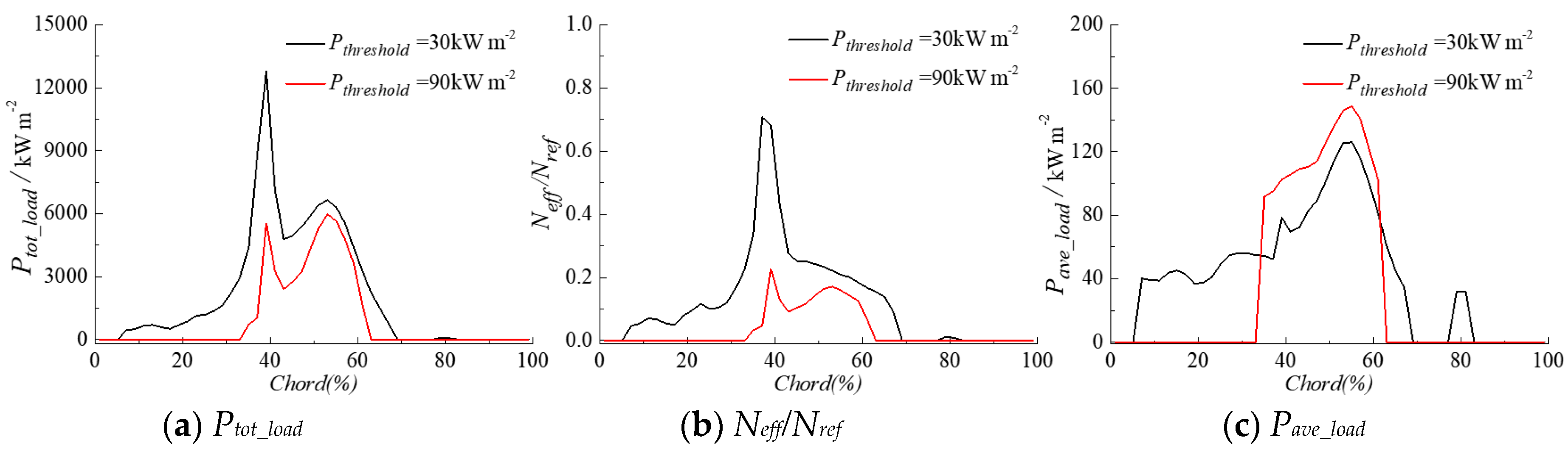
3.1. Influence of Driving Pressure Definition

The numerical results from two consecutive shedding cycles have been selected to calculate P_load on the hydrofoil surface with the different cavitation models and the obtained results have been plotted in Figure 5.

The top graphs in Figure 5 have been obtained considering p_d as the flow field instantaneous pressure, p(t). Conversely, the bottom graphs have been obtained considering p_d as the averaged pressure over ten cycles, $\overline{p}$. It can be observed that the space-time distributions of P_load on the suction side are different depending on which value has been used. For example, when taking the results obtained with the Sauer model, a region with high P_load has been predicted from 20% to 65% of the chord using $\overline{p}$ in the initial time ranges of each cycle from 0.2 to 0.45 T/T_ref and from 1.2 to 1.45 T/T_ref. It is observed that using p(t) the calculations can only capture a high P_load during a very short instant around 1.45 T/T_ref. Moreover, the amplitude of P_load is also different even though the attack occurs in a similar time-space region. Another large amplitude of P_load has been found with the use of both p(t) and $\overline{p}$ on a location around 40% of the chord from 0.45 to 1.0 T/T_ref for the first cycle and from 1.45 to 2.0 T/T_ref for the second cycle. However, this amplitude was higher when taking $\overline{p}$ as the driving pressure. To finish, similar differences have also been found when comparing the results of the other two cavitation models.

To understand such differences, the obtained $\dot{m}$ from vapor to water has been presented in Figure 6 for the second cycle at various relative instants, T/T_ref, marked with dotted lines in Figure 5b. Three stages of the cavity shedding process can be roughly identified. Firstly, the formation of the sheet cavity and its detachment occurs from 1.0 to 1.2 at the initial stage of the shedding process. Figure 6a,b at instants 1.0 and 1.1, respectively, show how the main sheet cavity detaches due to the re-entrant jet and then how a cloud cavity forms and begins to be convected downstream. The second stage ranges from 1.2 to 1.45 and corresponds to the collapse of the cloud cavity. In Figure 6c,d, it can be seen at instant 1.3 how the cloud cavity flows downstream and starts to collapse. Afterwards, the final collapse occurs at instant 1.44. Finally, the stage from 1.45 to 2.0 corresponds to the new growth and formation of the attached sheet cavity. As shown in Figure 6e,f, the sheet cavity reaches its maximum length and then a stagnation point at its closure region forms because the flow over the cavity turns towards the surface. This stagnation point creates a high pressure region which drives the upstream re-entrant jet below the attached cavity and triggers the collapse of the small vapor structures detached at the rear part of the sheet.

The results obtained using both p(t) and $\overline{p}$ have been plotted on the left- and right-hand sides of Figure 7 for comparison. In particular, the corresponding distributions of p(t) and $\overline{p}$, the distribution of P_den as well as the evolution of P_load on the hydrofoil surface along chord (red line) have been plotted at different instants. Moreover, the isolines of α_v = 0.1 (black lines) have been superimposed to those graphs to show the location of the main vapor cavities. From a general overview, it can be confirmed that the value of p_d has a significant influence on the results.

The results presented in Figure 6a at instant 1.0 show that the highest condensation processes take place at both ends of the attached cavity. In Figure 7, it is also confirmed that the values of p(t) in the condensation regions at this instant are higher than the corresponding values of $\overline{p}$. It can be seen that a higher P_den is predicted on the fluid using p(t), and correspondingly it results in a higher P_load on the hydrofoil surface. Likewise, at instant 1.1, the p(t) in the condensation region is also higher than $\overline{p}$, leading to a locally higher P_load. However, this is not a reliable result because, at this stage, when the sheet cavity is transformed into a cloud cavity, no strong collapses are expected to occur.

The results presented in Figure 6c at instant 1.3 show condensation regions located on the margin of the cloud cavity because the pressure in its outer region is definitely higher than that within its interior as shown in Figure 7c. Moreover, p(t) is very low and even almost equal to the vapor pressure inside the cloud cavity region marked by the isoline, which implies that the pressure difference between the driving pressure and vapor pressure is close to zero. As a result, a very low aggressiveness on the hydrofoil surface is predicted. On the other hand, the use of $\overline{p}$ determines a higher P_den and P_load at the condensation region.

The final cloud collapse takes place at instant 1.44, as shown in Figure 6d and Figure 7d, when a local value of p(t) over 1 MPa is predicted inducing the maximum values of P_den and P_load. However, this instantaneous pressure peak is the consequence of the final collapse but it is not the pressure source driving the cavity collapse. Moreover, the appearance of this local pressure peak is considered by Bensow et al., [37] to be a spurious effect of the numerical calculation. In contrast, the P_den and P_load predicted using $\overline{p}$ are much lower because the $\overline{p}$ levels are significantly smaller than the p(t) ones.

Finally, the area with the highest erosion power is mainly concentrated on the closure region of the sheet cavity as shown in Figure 7e at instant 1.6. In addition, a small cavity also appears after the final collapse of the cloud cavity due to the vortex rebound [38]. Comparing the results predicted using p(t) or $\overline{p}$, the latter gives higher P_den and P_load because its level on the condensation area is higher than for the former. Similarly, the results at instant 1.8 allow us to verify the previous observations.

Figure 8 shows the accumulated P_{tot_load} levels along the hydrofoil chord during one shedding cycle from instant 1 to 2 using Equation (23) with P_threshold equal to zero. It is observed that P_{tot_load} along the chord is much lower when using p(t) than $\overline{p}$, with the exception of a small region near the leading edge when using the Zwart and the Sauer models. Another observation is that the P_{tot_load} levels near the leading edge are even higher than those on the region where the cloud cavity collapses when using p(t). As already discussed before, this is because p(t) gives a higher P_den and P_load during the transition from sheet to cloud cavity but underestimates P_den during the cloud cavity collapse because the pressure difference between p(t) and vapor pressure is close to zero. Therefore, the results given by p(t) are not reasonable because they are in contradiction with the experimental results presented in Figure 2 proving that no significant erosion occurs along the chord in the range from 0 to 20%. Meanwhile, strong erosion is found downstream of the cavity closure region. In summary, it is confirmed that the cavitation erosion prediction results are sensitive to the definition of the driving pressure, and that the results obtained with $\overline{p}$ seem to be more in agreement with the experiments. Consequently, they will be taken into account in the following sections.

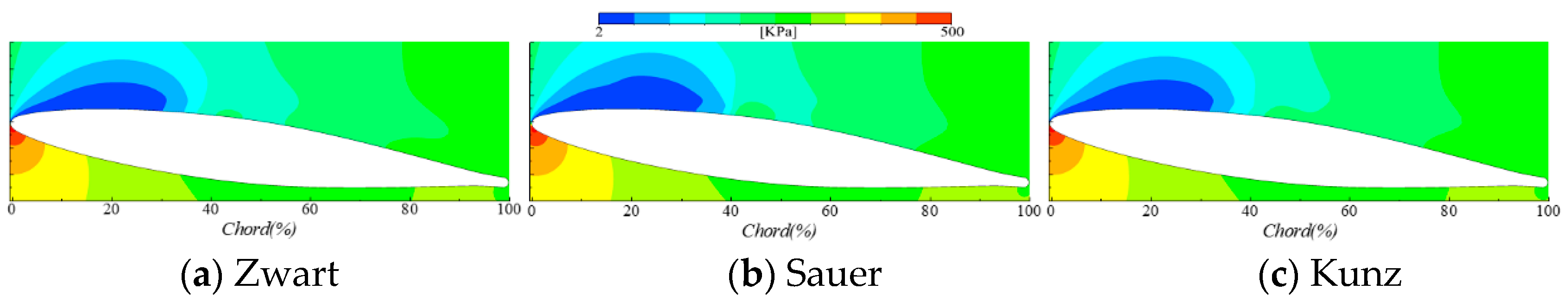
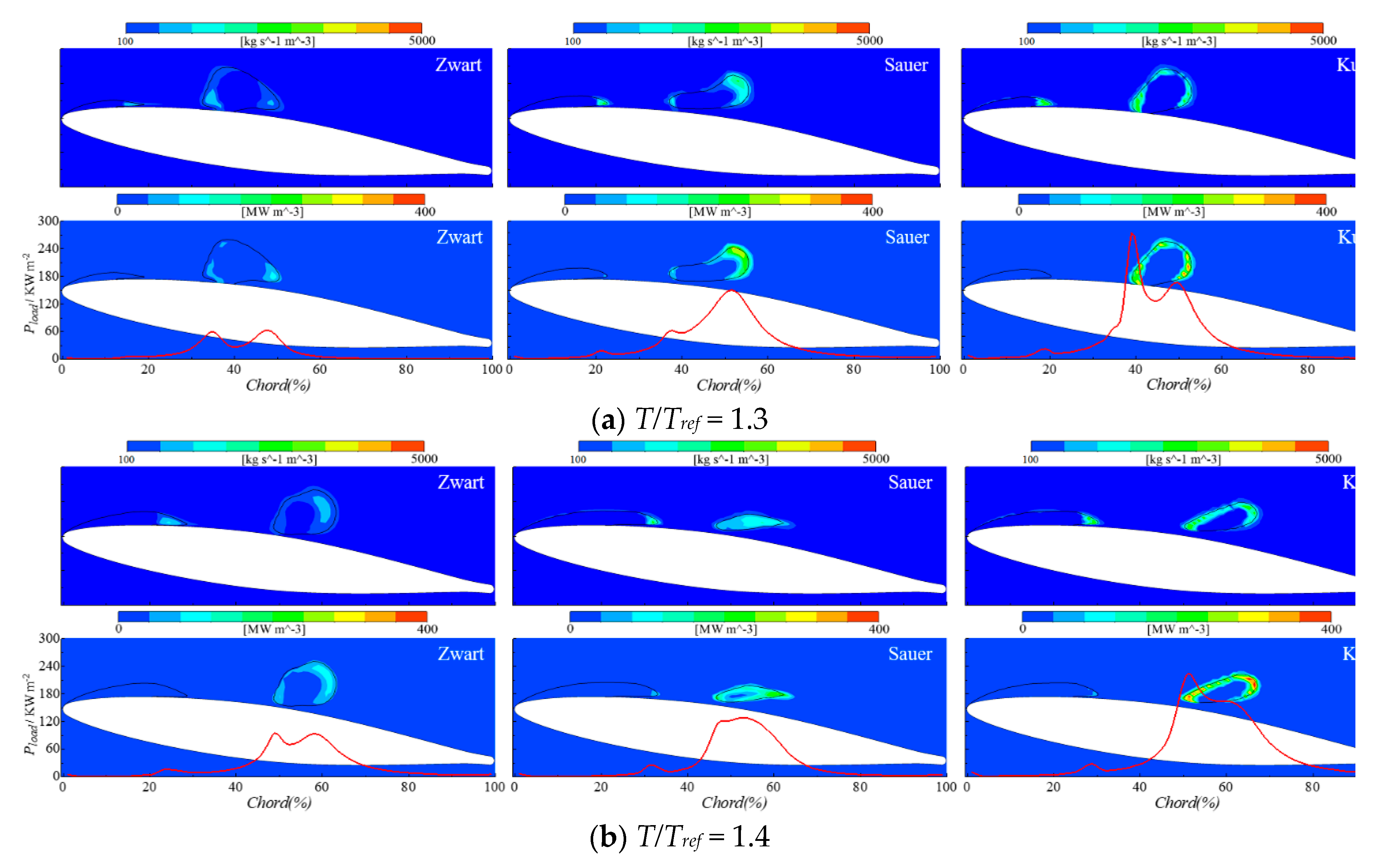
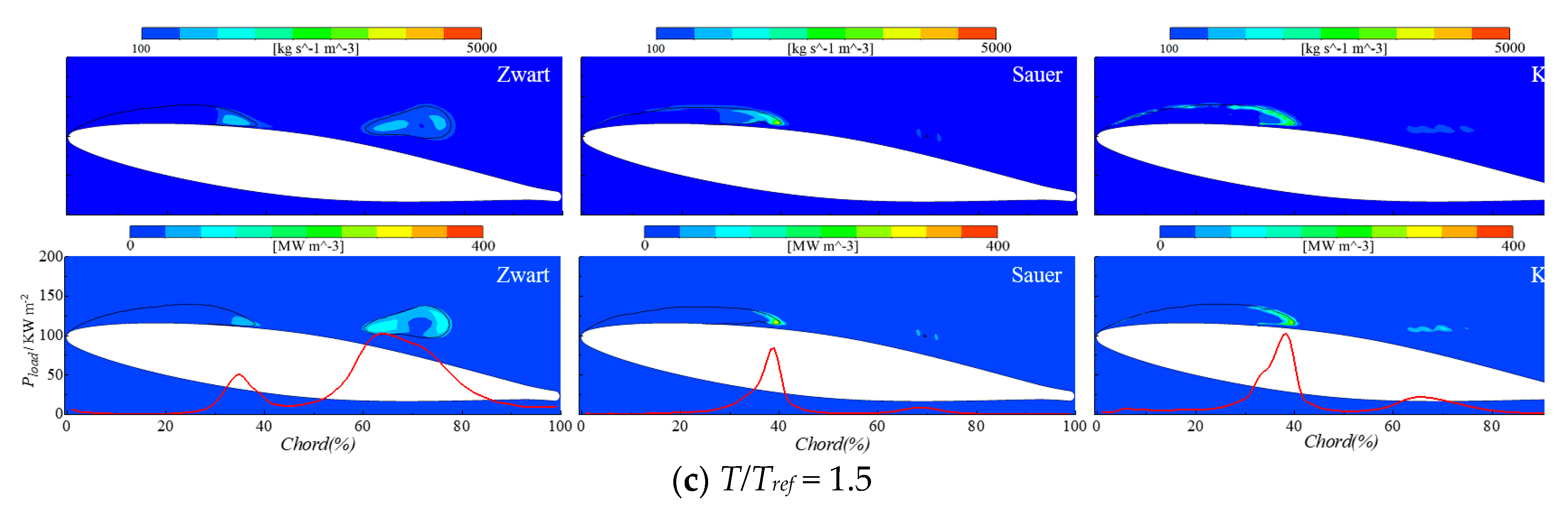
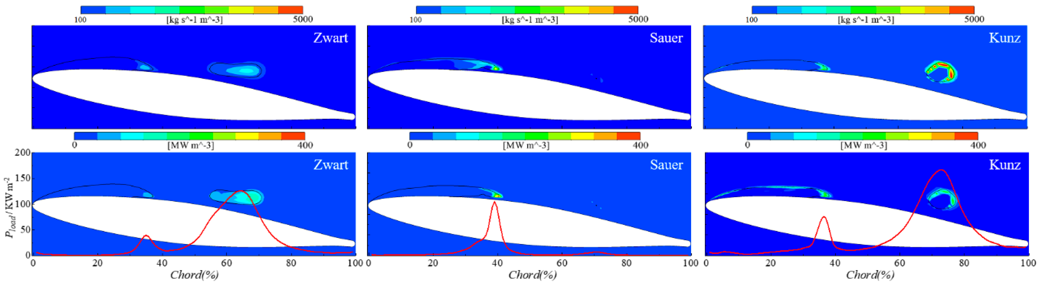
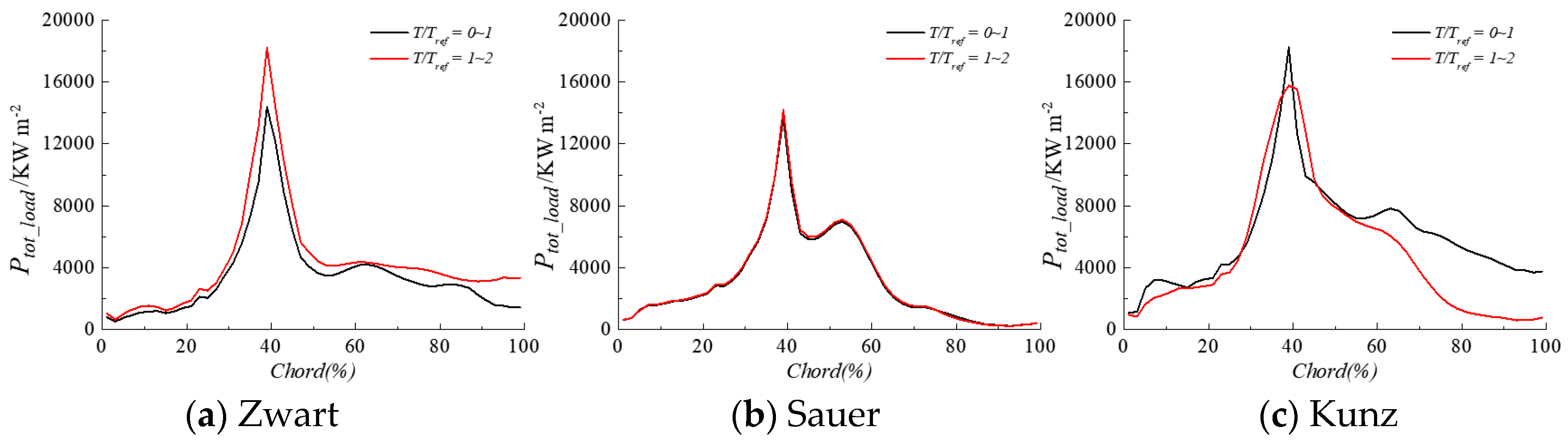
3.2. Influence of Cavitation Model

Figure 9 demonstrates that the contours of $\overline{p}$ obtained with the different cavitation models are similar, which reinforces the assumption that the study of the influence of the cavitation model on P_den and P_load can be done using $\overline{p}$ as driving pressure.

Figure 10 presents the contours of condensation $\dot{m}$ and P_den at different instants of the shedding process obtained with the Zwart, Sauer and Kunz cavitation models, as well as the evolution of P_load on the hydrofoil surface along the chord.

In Figure 10a, the Zwart model predicts a cloud cavity at instant 1.3 with low condensation rate on its outer region and a maximum P_load of about 60 kWm⁻² which is the lowest figure compared to the other models. On the contrary, the Sauer and the Kunz models predict a smaller cavity volume and a higher P_load induced by the higher condensation rate on the outer region of the cloud. More specifically, the Kunz model predicts the highest P_load of about 240 kW m⁻² at 40% of the chord because a part of the condensation region of the cloud cavity is much closer to the hydrofoil surface than in the rest of results. Similarly, the Zwart model predicts again the smallest condensation rate and P_load at instant 1.4. The other two models predict a relatively higher intensity especially for the Kunz one. At instant 1.5, the cloud cavity still presents a large volume with the Zwart model, meanwhile with the Sauer model the cavity already vanishes at instant 1.44, as shown in Figure 6d, and it reappears with a very small volume due to the collapse rebound. With the Kunz model, the cloud cavity finishes its final collapse at this particular instant. This indicates that the final collapse occurs at different instants and at different chord locations depending on the cavitation model. Furthermore, the collapse process predicted with the Zwart model creates a lower P_load than the rest. Comparing Figure 6d and Figure 10c, it can be seen that the Sauer model predicts a much higher condensation rate than with the Kunz model when the final collapse occurs, which leads to a higher P_den and P_load, as shown in Figure 7d.

Figure 11 shows the results at instant 0.5 corresponding to an analogous situation to the one observed at instant 1.5 presented in Figure 10c. By comparing these results, it can be seen that the cavity behavior differs between the two consequent cycles depending on the cavitation model being used. The cavity topologies at these two instants are very similar with the Sauer model, showing that the sheet cavity has reached its maximum length with a high P_load at its closure region and that a very small cloud cavity appears at 70% of the chord inducing a small P_load. Likewise, the cavity behavior and the P_load provided by the Zwart model at these two instants are also similar. However, the results for the Kunz model are different since there is a cloud with a larger volume of vapor that induces the maximum P_load at 75% of the chord at instant 0.5, which cannot be observed at instant 1.5 in Figure 10c. Similarly, the space-time distributions of P_load in Figure 5 are significantly different between the time span from 0 to 1 and from 1 to 2 for the Kunz model, meanwhile they are quite similar for the other two models. Consequently, it can concluded that the Zwart and Sauer models provide similar predictions of the erosion power in terms of erosion aggressiveness and location from cycle to cycle, while the Kunz model provides results that differ from cycle to cycle.

Figure 12 represents compares the values of P_{tot_load} without setting any threshold value for two consecutive shedding cycles obtained with the three cavitation models. With the Zwart model, a similar shape and amplitude of the P_{tot_load} distribution is found in both cycles although the second one gives a slightly higher intensity. With the Sauer model, the two cycles show exactly the same result. In contrast, with the Kunz model a significant difference is found in the second half of the chord. More specifically, P_{tot_load} drops with a faster rate towards a very small amplitude at 80% of the chord during the second cycle, meanwhile P_{tot_load} decreases more gradually and it is still significant even at the trailing edge during the first cycle. Note that similar differences between two consecutive cycles are also observed along the 10 cycles shown in Figure 5 for all the cavitation models.

Another conclusion that can be extracted from Figure 12 is that the cavitation model also influences the erosion distribution along the chord. More specifically, all three models give the maximum values of P_{tot_load} around 40% of the chord at the attached cavity closure region but they give different results at the cloud cavity collapse region. With the Zwart model, the collapses of the clouds, shown on the left hand side of Figure 10, are less intense and they take place close to the trailing edge presenting a low amplitude of P_{tot_load} from 50 to 100% of the chord. With the Sauer model, the cloud collapses are concentrated from 50 to 60% of the chord and the results show a small peak around 55% of the chord. With the Kunz model, the results are sensitive to the shedding cycle being considered. According to the experimental results presented in Figure 2, the main eroded area was located from 30 to the 70% of the chord and the maximum erosion was found from 40 to 50% of the chord. Based on these results, it can be concluded that the cavitation power distribution predicted by the Sauer model agrees more precisely with the experimental observations.

Based on the previous discussion, it can be stated that different cavitation models give different results of cavitation aggressiveness regarding the condensation $\dot{m}$, which determines the level of P_den, and regarding the cavity topology, which determines the efficiency of the transmission from P_den to P_load on the surface and the size and location of the area subjected to the highest P_{tot_load}. Nonetheless, it can be concluded that the Sauer model giver a more accurate prediction of cavitation aggressiveness than the rest.

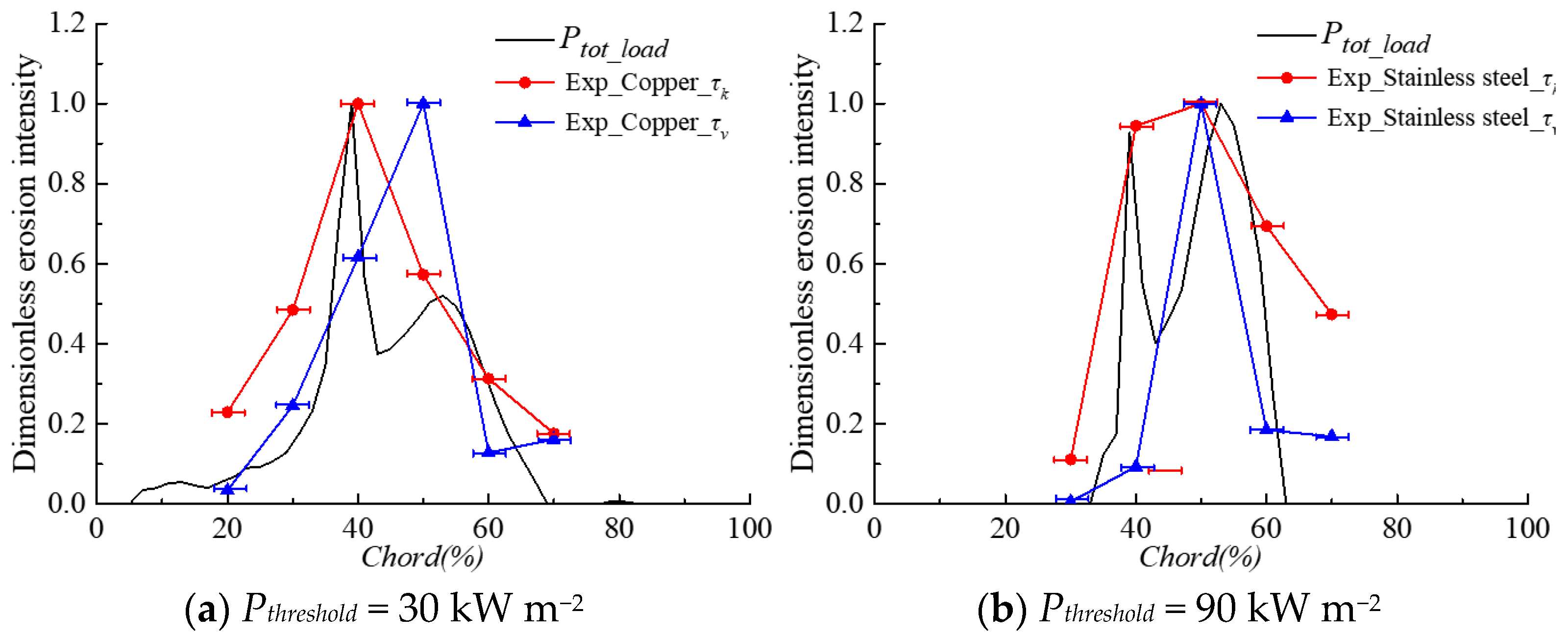
3.3. The Mechanism of Cavitation Erosion

In this section, the numerical results obtained with the Sauer model have been used to discuss the mechanisms of cavitation erosion based on the comparison with the experimental observations. For that, the second cycle results from instants 1 to 2 have been considered without any loss of generality because the Sauer model has shown a good repeatability for all the simulated shedding cycles.

Figure 12b shows that the maximum P_{tot_load} is found both at the closure region of the attached sheet cavity and at the location where the main cloud cavity collapses. Nevertheless, the calculation of P_{tot_load} without taking into account the fact that a P_threshold level exists is not an accurate method to estimate the actual erosion risk. Therefore, a P_threshold has been set to eliminate the contribution of low intensity collapses not being sufficiently high to cause material damage. For that, the number of effective time steps at which P_load is higher than P_threshold at any chord location, N_eff, has been considered to estimate the average erosive power load, P_{ave_load}, at each effective time step and hydrofoil position with the following expression:

$$P_{ave\_load}=\raisebox{1ex}{$P_{tot\_load}$}\!\left/ \!\raisebox{-1ex}{$N_{eff}$}\right.$$

(24)

If N_ref is the number of time steps in one cycle of duration T_ref, then the ratio N_eff/N_ref accounts for the percent time duration during one shedding cycle with P_load values higher than P_threshold.

In the present study, two P_threshold levels with values of 30 kW m⁻² and 90 kW m⁻² have been considered to investigate the influence of the particular material resistance to cavitation erosion and the corresponding distributions of P_{tot_load}, N_eff/N_ref and P_{ave_load} along the chord have been plotted in Figure 13. Note here that it can be assumed that the lower level of 30 kW m⁻² represents copper and that the level of 90 kW m⁻² represents stainless steel since there is no doubt that copper has a lower yield strength than stainless steel.

For P_threshold of 30 kW m⁻², the maximum values of P_{tot_load} and N_eff/N_ref are found at 40% of the chord but at this location P_{ave_load} is relatively small compared to the rest of values farther downstream. This is because small vapor structures are collapsing at the cavity closure region for a long time duration (0.7 T_ref) but they are individually inducing relatively small P_load. This prediction is in agreement with the experimental results that show a high pitting rate at this location but with a relatively small deformation volume rate. The second peak value of P_{tot_load} is located at 53% of the chord. In this case, N_eff/N_ref is around 0.2 while P_{ave_load} shows its maximum value. This indicates that, at the region of the cloud collapses, the erosion intensity is very high but its time duration during one cycle is relatively short. This is again in agreement with the experiment that shows a relatively smaller pitting rate but with the highest deformation volume rate in the same position.

When P_threshold increases to 90 kW m⁻², the strongest erosions are also predicted at the sheet cavity closure and at the location where the main clouds collapse. However, it can be seen in Figure 13a,b that P_{tot_load} and N_eff/N_ref decrease significantly in the sheet cavity closure region but only slightly in the cloud collapse region when compared with the results obtained with 30 kW m⁻². Now the maximum P_{tot_load} is located at around 53% of the chord instead of 40%, which is also in accordance with the experimental results for the stainless steel specimen that showed the highest pitting rate at around the 50%. These numerical predictions confirm the existence of a threshold level and the fact that it permits the correction of the estimation of the cavitation erosion risk based on the cavitation aggressiveness. Increasing P_threshold, the contribution to erosion of the small intensity collapses taking place during a long time at the sheet cavity closure is dampened but it does not affect the results at the cloud collapse region where the P_{tot_load} is very high and clearly above P_threshold.

Therefore, the setting of P_threshold is necessary to take into account the material resistance in the numerical prediction of cavitation erosion. Moreover, this is a concept that can also be used to explain the experimental observations found with different types of materials if it is assumed that it reproduces the effects of the material yield stress.

For example, the numerical P_{tot_load} and the experimental τ_n and τ_v have been normalized by their respective maxima along the chord and compared in Figure 14. It can be seen that the predicted results for P_threshold of 30 kW m⁻² compare well with the copper erosion measurements, and the ones for 90kW m⁻² compare well with stainless steel especially for the pitting rate observations. In addition, the numerical results show a zone with a low erosion intensity like a groove between the two maximum erosion picks for P_{tot_load}, which is due to the fact that in the simulations the boundary between the vapor and water phases is very well delimited whereas in reality these boundaries are quite unstable and the cavity wake is much fuzzier due to the flow turbulence [21].

Given the good results obtained with the present simulations, the Sauer model has been further used to investigate the effect of the free stream velocity on the cavitation erosion power.

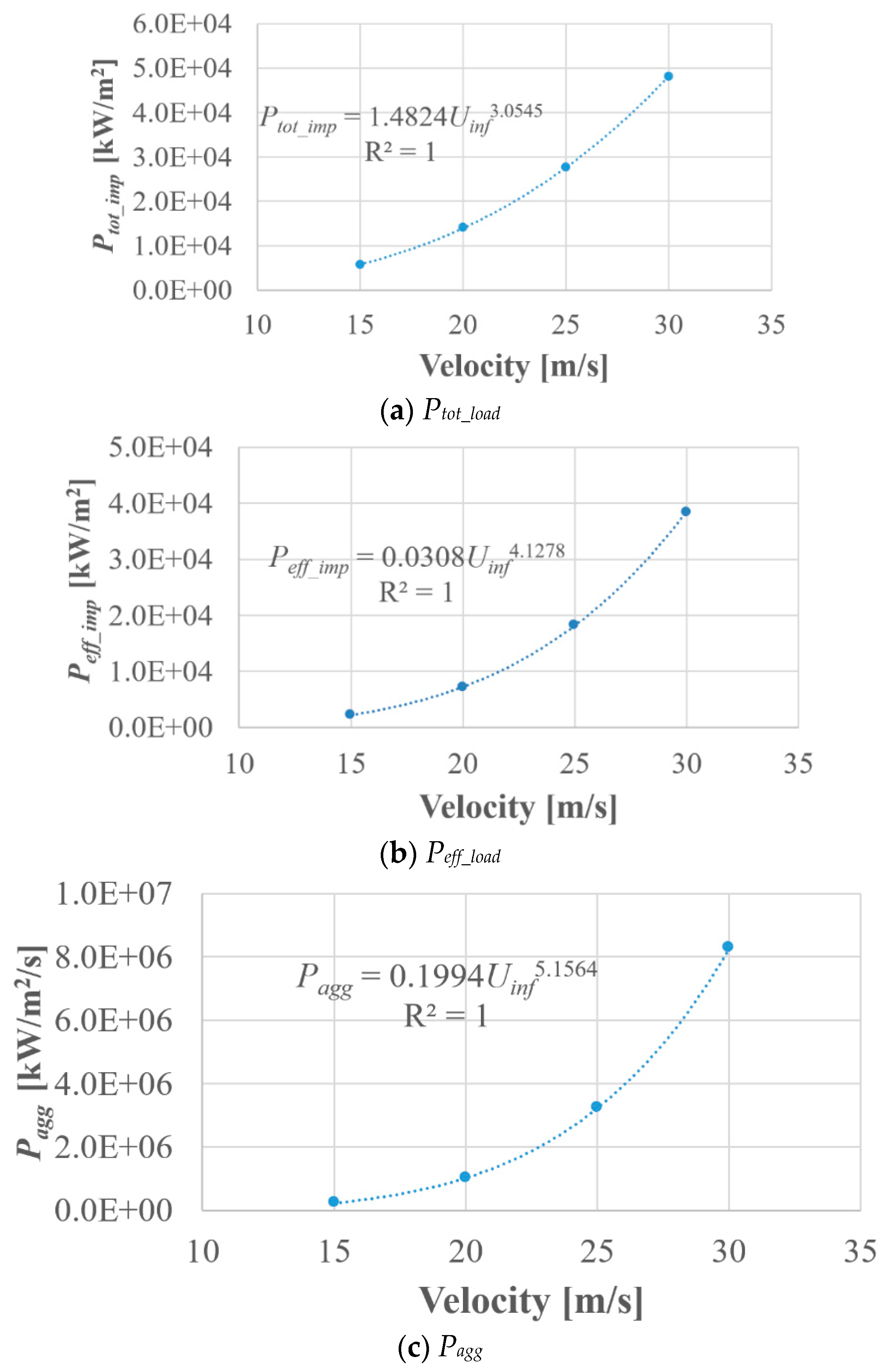
3.4. Free Stream Velocity Effects

Four different free stream water velocities, U_inf, have been simulated with the same numerical model corresponding to 15, 20, 25 and 30 m/s. The time step has been set inversely proportional to U_inf in order to keep the Courant number constant between all the simulations. In addition, the outlet pressure has been adjusted correspondingly in order to get always the same cavity length around the 40% of the chord as in the experiment. The model setup main parameters and the shedding frequencies calculated numerically and measured experimentally have been listed in

Table 3. Numerical and experimental shedding frequency results for the various flow conditions and numerical.

Uinf [m/s]	Time Step [s]	σexp	σ CFD	fexp [s−1]	fCFD [s−1]	fdev [%]
15	0.00004	1.55	1.55	96.1	106	10.3
20	0.00003	1.58	1.55	132.8	139	4.7
25	0.000024	1.60	1.55	175.5	177	0.8
30	0.00002	1.62	1.55	225.8	216	−4.3

. It can be seen that the simulations predict with good accurately the shedding frequencies for any U_inf with a maximum percent deviation of 10.3%. Similarly to the results shown in Figure 4b, the time signals of the total vapor volume are repeatable from cycle to cycle for all the cases. Finally, the driving pressure has been based on the averaged instantaneous pressures over ten shedding cycles.

To study the relationship between cavitation aggressiveness and flow velocity, the collapse efficiency proposed by Fortes-Patella et al., [39], η_collapse, has been used which quantifies the effective energy transfer between the potential power of the vapor volume and the actually erosive power. The value of η_collapse is dependent on the initial gas pressure inside the bubble, P_g0, and the environment pressure, P_∞, but it is weakly dependent on the initial vapor volume so it can be calculated as:

$${\eta }_{collapse}=0.029{\left(P_{g0}/P_{\infty }\right)}^{-0.54}$$

(25)

Equation (25) shows that, for a given P_g0, the efficiency is higher the higher is P_∞ which means that for a given cavitation number, the collapses will release more energy for higher U_inf. In the present work, P_g0 has been taken as 1500 Pa and P_∞ has been calculated with the numerical cavitation number as done in [39]. Therefore, η_collapse is a constant coefficient depending on U_inf as shown in

Table 4. Numerically calculated indicators of cavitation erosion for different flow velocities.

Uinf [m/s]	Ptot_load [kW m−2]	P∞ [Pa]	Pg0 [Pa]	ηcollapse [%]	Peff_load_ [kW m−2]	fCFD [s−1]	Pagg [kW m−2 s−1]
15	5792	176,026	1500	38.0	2202	106	233,385
20	13,963	311,380	1500	51.7	7222	139	1,003,915
25	27,711	485,406	1500	65.7	18,216	177	3,224,249
30	48,033	698,105	1500	80.0	38,421	216	8,298,901

. Then, the actual effective erosion power load, P_{eff_load}, can be calculated as:

$$P_{eff\_load}=P_{tot\_load}{\eta }_{collapse}$$

(26)

Since the experimentally obtained Strouhal number at different U_inf is constant with a value around 0.28 (see Table 1), the shedding frequency will increase linearly with U_inf and the collapsing frequency on the hydrofoil will also increase. Therefore, the cavitation erosion aggressiveness per unit time, P_agg, can defined as:

$$P_{agg}=P_{eff\_load}/T=P_{eff\_load}\cdot f$$

(27)

All the calculated values of the various cavitation erosion indicators defined in this section have been listed in Table 4 and plotted in Figure 15, where several power law relations between them and U_inf have been found. Note that P_{tot_load} and P_{eff_load} are the accumulated potential power and the accumulated effective power for one complete shedding cycle, respectively, and P_agg is the accumulated effective power per unit time. The maximum P_{tot_load} along the chord, which is found at 40% of the chord for each U_inf because of no threshold has been considered, has also been selected to quantify the flow velocity effects.

As observed in Figure 15a, P_{tot_load} increases approximately as U_inf to the third power for one shedding cycle, which is in accordance with the numerical results obtained by other researchers like Carrat et al., [23], Leclercq et al., [24] and Melissaris et al., [27], although they did not take into account the collapse efficiency. As observed in Figure 15b, P_{eff_load} increases approximately as U_inf to the fourth power when considering the efficiency which is in accordance with the numerical results obtained by Fortes-Patella et al. [39]. Finally, because the shedding frequency increases with the flow velocity, P_agg increases approximately as U_inf to the fifth power as shown in Figure 15c but this curve might rise faster, i.e., present a higher exponent, because the shedding frequency has been slightly overestimated for the lowest U_inf and underestimated for the highest U_inf in the present calculations. In addition, the experimental cavitation numbers are higher for the higher velocities than those in the numerical model, which implies higher environment pressures and higher collapse efficiencies for higher velocities. Consequently, the erosion rate may increase with an exponent higher than 5, which would be in agreement with the experimental investigations by Dular et al., [40,41] who found that the erosion damage followed a power law with n values from 5 to 8.

4. Conclusions

In the present study, the dynamic behavior and the erosion power of unsteady cloud cavitation on a 2D hydrofoil has been investigated numerically based on an energy balance approach. The influences of the driving pressure and of the cavitation model have been discussed in detail. The numerical prediction of erosion is in agreement with the experimental measurements and with the main erosion mechanisms. Moreover, the influence of flow velocity on erosion power has been quantified. As a result, the following conclusions have been obtained:

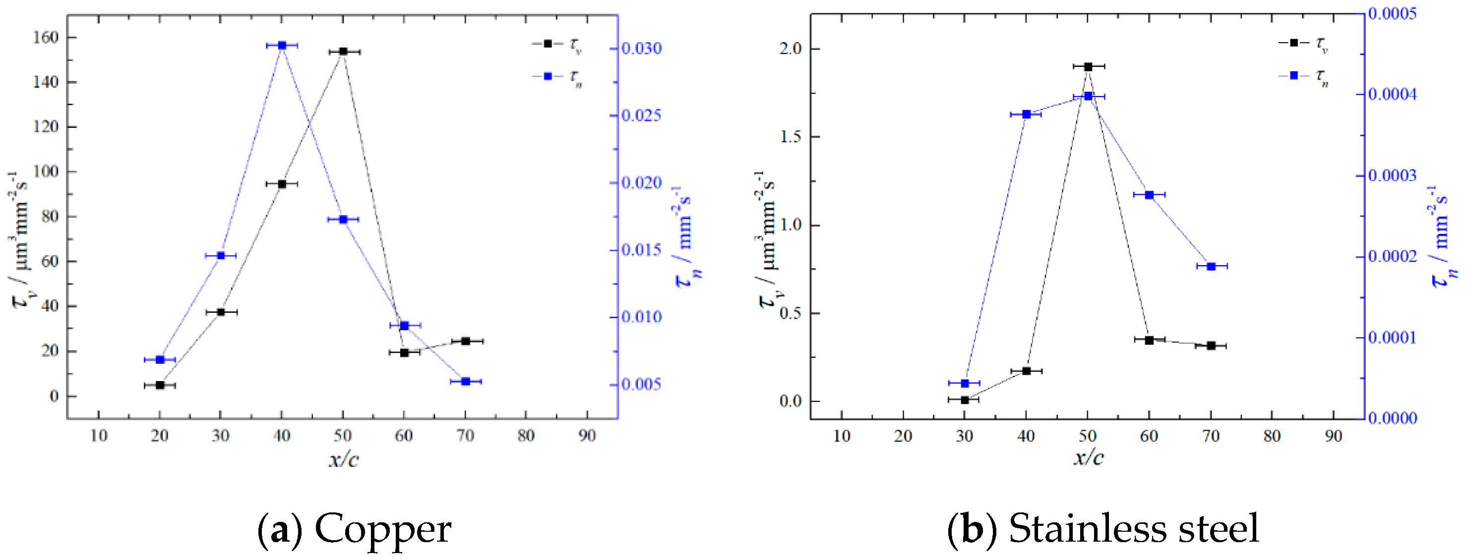
• The selection of the driving pressure to estimate the power of the cavity collapse has a significant effect on the space-time distribution of the cavitation aggressiveness on the hydrofoil surface. The use of the average pressure gives more similar results to the experiment than the use of the instantaneous pressure.
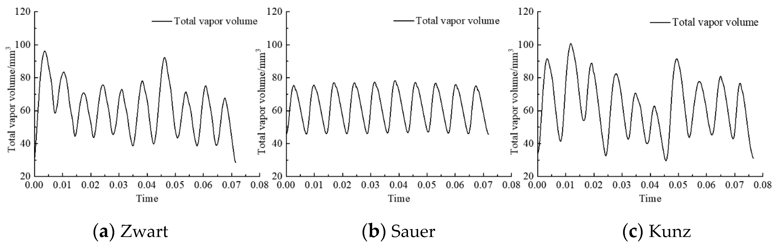
• The cavitation model influences significantly the power loaded on the hydrofoil surface both in terms of magnitude and spatial distribution along the chord. For the cases considered in the present study, the Sauer model performs better than the Kunz and Zwart ones.
• Two main erosion mechanisms have been predicted that are in good agreement with experimental observations. One is induced by the high frequency of low-intensity collapses taking place at the closure region of the main sheet cavity attached to the hydrofoil surface. The other one is induced by the low frequency and high intensity collapses of the shed cloud cavities.
• Power laws have been obtained that permit the calculation of the erosive cavitation intensity as a function of the flow velocity by taking into account the collapse efficiency and the shedding frequency. More specifically, the effective power load law grows with an exponent of 4, and the erosion aggressiveness per unit time grows with an exponent of 5.

References

1. Kim, K.H.; Chahine, G.; Franc, J.P.; Karimi, A. Advanced Experimental and Numerical Techniques for Cavitation Erosion Prediction; Springer: New York, NY, USA, 2014. [Google Scholar]
2. Li, Z.R. Assessment of cavitation erosion with a multiphase Reynolds-Averaged Navier-Stokes method. Ph.D. Thesis, Delft University of Technology, Wageningen, The Netherlands, 2012. [Google Scholar]
3. Hsiao, C.T.; Jayaprakash, A.; Kapahi, A.; Choi, J.K.; Chahine, G.L. Modelling of material pitting from cavitation bubble collapse. J. Fluid Mech. 2014, 755, 142–175. [Google Scholar] [CrossRef] [Green Version]
4. Fivel, M.; Franc, J.P.; Chandra Roy, S. Towards numerical prediction of cavitation erosion. Interface Focus 2015, 5, 20150013. [Google Scholar] [CrossRef] [PubMed]
5. Roy, S.C.; Franc, J.P.; Pellone, C.; Fivel, M. Determination of cavitation load spectra–Part 1: Static finite element approach. Wear 2015, 344, 110–119. [Google Scholar] [CrossRef] [Green Version]
6. Roy, S.C.; Franc, J.P.; Pellone, C.; Fivel, M. Determination of cavitation load spectra–Part 2: Dynamic finite element approach. Wear 2015, 344, 120–129. [Google Scholar] [CrossRef] [Green Version]
7. Joshi, S.; Franc, J.P.; Ghigliotti, G.; Fivel, M. SPH modelling of a cavitation bubble collapse near an elasto-visco-plastic material. J. Mech. Phys. Solids. 2019, 125, 420–439. [Google Scholar] [CrossRef] [Green Version]
8. Joshi, S.; Franc, J.P.; Ghigliotti, G.; Fivel, M. Bubble collapse induced cavitation erosion: Plastic strain and energy dissipation investigations. J. Mech. Phys. Solids. 2020, 134, 103749. [Google Scholar] [CrossRef]
9. Ochiai, N.; Iga, Y.; Nohmi, M.; Ikohagi, T. Numerical prediction of cavitation erosion intensity in cavitating flows around a Clark Y 11.7% hydrofoil. J. Fluid Sci. Tech. 2010, 5, 416–431. [Google Scholar] [CrossRef] [Green Version]
10. Wang, H.; Zhu, B. Numerical prediction of impact force in cavitating flows. Trans. ASME J. Fluids Eng. 2010, 132, 101301. [Google Scholar] [CrossRef]
11. Eskilsson, C.; Bensow, R.E.; Kinnas, S. Estimation of cavitation erosion intensity using CFD: Numerical comparison of three different methods. In Proceedings of the 4th International Symposium on Marine Propulsors, Austin, TX, USA, 31 May–4 June 2015. [Google Scholar]
12. Schnerr, G.H.; Sezal, I.H.; Schmidt, S.J. Numerical Investigation of Three-Dimensional Cloud Cavitation with Special Emphasis on Collapse Induced Shock Dynamics. Phys. Fluids. 2008, 20, 040703. [Google Scholar] [CrossRef]
13. Mihatsch, M.S.; Schmidt, S.J.; Adams, N.A. Cavitation erosion prediction based on analysis of flow dynamics and impact load spectra. Phys. Fluids. 2015, 20, 103302. [Google Scholar] [CrossRef]
14. Blume, M.; Skoda, R. 3D flow simulation of a circular leading edge hydrofoil and assessment of cavitation erosion by the statistical evaluation of void collapses and cavitation structures. Wear 2019, 428, 457–469. [Google Scholar] [CrossRef]
15. Nohmi, M.; Ikohagi, T.; Iga, Y. Numerical Prediction Method of Cavitation Erosion. In Proceedings of the ASME 2008 Fluids Engineering Division Summer, Jacksonville, FL, USA, 10–14 August 2008. [Google Scholar]
16. Li, Z.R.; Pourquie, M.; van Terwisga, T. Assessment of cavitation erosion with a URANS method. Trans. ASME J. Fluids Eng. 2014, 136, 041101. [Google Scholar] [CrossRef]
17. Fortes-Patella, R.; Reboud, J.L.; Briancon-Marjollet, L. A phenomenological and numerical model for scaling the flow agressiveness in cavitation erosion. In Proceedings of the EROCAV Workshop, Val de Reuil, France, May 2004. [Google Scholar]
18. Patella, R.F.; Archer, A.; Flageul, C. Numerical and experimental investigations on cavitation erosion. In Proceeding of the 26th IAHR Symposium on Hydraulic Machinery and Systems, Beijing, China, 19–23 August 2012. [Google Scholar]
19. Koukouvinis, P.; Bergeles, G.; Gavaises, M. A cavitation aggressiveness index within the Reynolds averaged Navier Stokes methodology for cavitating flows. J. Hydrodyn. 2015, 27, 579–586. [Google Scholar] [CrossRef] [Green Version]
20. Ponkratov, D.; Caldas, A. Prediction of Cavitation Erosion by Detached Eddy Simulation (DES) and its Validation against Model and Ship Scale Results. In Proceeding of the 4th International Symposium on Marine Propulsors, Austin, TX, USA, 31 May–4 June 2015. [Google Scholar]
21. Dular, M.; Coutier-Delgosha, O. Numerical modelling of cavitation erosion. Int. J. Numer. Methods Fluids. 2009, 61, 1388–1410. [Google Scholar] [CrossRef]
22. Peters, A.; Sagar, H.; Lantermann, U.; el Moctar, O. Numerical modelling and prediction of cavitation erosion. Wear 2015, 338, 189–201. [Google Scholar] [CrossRef]
23. Carrat, J.B.; Fortes-Patella, R.; Franc, J.P. Assessment of cavitating flow aggressiveness on a hydrofoil: Experimental and numerical approaches. In Proceedings of the ASME 2017 Fluids Engineering Division Summer Meeting, Waikoloa, HI, USA, 30 July–3 August 2017. [Google Scholar]
24. Leclercq, C.; Archer, A.; Fortes-Patella, R.; Cerru, F. Numerical cavitation intensity on a hydrofoil for 3D homogeneous unsteady viscous flows. Int. J. Fluid Mach. Syst. 2017, 10, 254–263. [Google Scholar] [CrossRef]
25. Melissaris, T.; Bulten, N.; van Terwisga, T.J.C. On Cavitation Aggressiveness and Cavitation Erosion on Marine Propellers using a URANS Method. In Proceeding of the 10th International Symposium on Cavitation, Baltimore, MD, USA, 14–16 May 2018. [Google Scholar]
26. Schenke, S.; van Terwisga, T.J. An energy conservative method to predict the erosive aggressiveness of collapsing cavitating structures and cavitating flows from numerical simulations. Int. J. Multiph. Flow 2019, 111, 200–218. [Google Scholar] [CrossRef] [Green Version]
27. Melissaris, T.; Bulten, N.; van Terwisga, T.J. On the Applicability of Cavitation Erosion Risk Models With a URANS Solver. Trans. ASME J. Fluids Eng. 2019, 141, 101104. [Google Scholar] [CrossRef] [Green Version]
28. Leclercq, C. Simulation numérique du chargement mécanique en paroi généré par les écoulements cavitants, pour application à l’usure par cavitation des pompes centrifuges. Ph.D. Thesis, Université Grenoble Alpes, Grenoble Alpes, France, 2017. [Google Scholar]
29. Escaler, X.; Farhat, M.; Egusquiza, E.; Avellan, F. Dynamics and intensity of erosive partial cavitation. Trans. ASME J. Fluids Eng. 2007, 129, 886–893. [Google Scholar] [CrossRef] [Green Version]
30. Couty, P. Physical investigation of cavitation vortex collapse. Ph.D. Thesis, EPFL, Lausanne, Switzerland, 2002. [Google Scholar]
31. Geng, L.; Escaler, X. Assessment of RANS turbulence models and Zwart cavitation model empirical coefficients for the simulation of unsteady cloud cavitation. Eng. Appl. Comp. Fluid Mech. 2020, 14, 151–167. [Google Scholar] [CrossRef]
32. Coutier-Delgosha, O.; Fortes-Patella, R.; Reboud, J.L. Evaluation of the turbulence model influence on the numerical simulations of unsteady cavitation. Trans. ASME J. Fluids Eng. 2003, 125, 38–45. [Google Scholar] [CrossRef] [Green Version]
33. Zwart, P.J.; Gerber, A.G.; Belamri, T. A Two-Phase Flow Model for Predicting Cavitation Dynamics. In Proceedings of the International Conference on Multiphase Flow, Yokohama, Japan, 30 May–4 June 2004. [Google Scholar]
34. Schnerr, G.H.; Sauer, J. 2001 Physical and Numerical Modeling of Unsteady Cavitation Dynamics. In Proceedings of the 4th International Conference on Multiphase Flow, New Orleans, LA, USA, 27 May–1 June 2001. [Google Scholar]
35. Kunz, R.F.; Boger, D.A.; Stinebring, D.R.; Chyczewski, T.S.; Lindau, J.W.; Gibeling, H.J.; Venkateswaran, S.; Govindan, T.R. A Preconditioned Navier-Stokes Method for Two-Phase Flows with Application to Cavitation Prediction. Comput. Fluids 2000, 29, 849–875. [Google Scholar] [CrossRef]
36. Leclercq, C.; Archer, A.; Fortes-Patella, R. 2016 Numerical investigations on cavitation intensity for 3d homogeneous unsteady viscous flows. In Proceeding of the 28th IAHR Symposium on Hydraulic Machinery and Systems, Grenoble, France, 4–8 July 2016. [Google Scholar]
37. Asnaghi, A.; Feymark, A.; Bensow, R.E. Numerical investigation of the impact of computational resolution on shedding cavity structures. Int. J. Multiph. Flow 2018, 107, 33–50. [Google Scholar] [CrossRef]
38. Lu, N.X.; Bensow, R.E.; Bark, G. Indicators of erosive cavitation in numerical simulations. In Proceeding of the 7th international workshop on ship hydrodynamics, Shanghai, China, 16–19 September 2011. [Google Scholar]
39. Fortes-Patella, R.; Challier, G.; Reboud, J.L.; Archer, A. Energy Balance in Cavitation Erosion: From Bubble Collapse to Indentation of Material Surface. Trans. ASME J. Fluids Eng. 2013, 135, 011303. [Google Scholar] [CrossRef]
40. Bachert, B.; Dular, M.; Baumgarten, S.; Ludwig, G.; Stoffel, B. Experimental investigations concerning erosive aggressiveness of cavitation at different test configurations. In Proceedings of the ASME Heat Transfer/Fluids Engineering Summer Conference, Westin Charlotte, NC, USA, 11–15 July 2004. [Google Scholar]
41. Dular, M.; Sirok, B.; Stoffel, B. Influence of gas content in water and flow velocity on cavitation erosion aggressiveness. Stroj. Vestn. J. Mech E. 2005, 51, 132–145. [Google Scholar]
Figure 1. 2D computational domain with named boundaries and frame of reference.
Applsci 10 05184 g001
Figure 2. Experimentally measured mean volume deformation rate (black left axis) and mean pitting rate (blue right axis).
Applsci 10 05184 g002
Figure 3. Schematic of the point power source where the cavity collapse takes place and its path to the point on the hydrofoil surface that will be loaded by the emitted power.
Applsci 10 05184 g003
Figure 4. Numerically predicted time evolution of the total vapor volume in the fluid domain with the different cavitation models.
Applsci 10 05184 g004
Figure 5. Comparison of calculated power load per unit area, Pload, on the hydrofoil surface based on instantaneous pressure, p(t) (top) and on average pressure,   p ¯ (bottom).
Applsci 10 05184 g005
Figure 6. Contours of m ˙ from vapor to water at different instants of the shedding cycle. Black isolines of αv = 0.1 show the locations of the main vapor cavities at each instant.
Applsci 10 05184 g006
Figure 7. Contours of p(t) (top left), p ¯ (top right), Pden and amplitude of Pload along the chord (bottom left and right) obtained using p(t) (left) and p ¯ (right). Red lines showing the value of the power load on the surface along the chord. Black isolines of αv = 0.1 show the locations of the main vapor cavities at each instant.
Applsci 10 05184 g007aApplsci 10 05184 g007b
Figure 8. The accumulated total power load during the second shedding cycle predicted using p(t) or p ¯ with different cavitation models.
Applsci 10 05184 g008
Figure 9. Contours of p ¯ predicted with the different cavitation models.
Applsci 10 05184 g009
Figure 10. Results obtained with the Zwart (left), Sauer (middle) and Kunz (right) models at different instants comprising contours of m ˙ from vapor to water (top) and of Pden, and value of Pload on the surface along the chord (red line in bottom graphs). Black isolines of αv = 0.1 show the location of the main vapor cavities at each instant.
Applsci 10 05184 g010aApplsci 10 05184 g010b
Figure 11. Results obtained with the Zwart (left), Sauer (middle) and Kunz (right) models at instant T/Tref = 0.5 comprising contours of m ˙ from vapor to water (top) and contours of power density and value of the power load on the surface along the chord (red line in bottom graphs). Black isolines of αv = 0.1 showing the location of the main vapor cavities at each instant.
Applsci 10 05184 g011
Figure 12. Comparison of Ptot_load distribution obtained for the first (black line) and second (red line) shedding cycles with the different cavitation models.
Applsci 10 05184 g012
Figure 13. Distribution of Ptot_load, Neff/Nref and Pave_load along the chord for Pthreshold levels of 30 and 90 kW m−2.
Applsci 10 05184 g013
Figure 14. Comparison of dimensionless erosion intensity indicators between numerical and experimental results.
Applsci 10 05184 g014
Figure 15. Predicted cavitation erosion intensity indicators at 40% of the chord as a function of flow velocity.
Applsci 10 05184 g015