A Decision-Support Model for Additive Manufacturing Scheduling Using an Integrative Analytic Hierarchy Process and Multi-Objective Optimization

Abstract

Additive manufacturing (AM) became widespread through several organizations due to its benefits in providing design freedom, inventory improvement, cost reduction, and supply chain design. Process planning in AM involving various AM technologies is also complicated and scarce. Thus, this study proposed a decision-support tool that integrates production and distribution planning in AM involving material extrusion (ME), stereolithography (SLA), and selective laser sintering (SLS). A multi-objective optimization approach was used to schedule component batches to a network of AM printers. Next, the analytic hierarchy process (AHP) technique was used to analyze trade-offs among conflicting criteria. The developed model was then demonstrated in a decision-support system environment to enhance practitioners’ applications. Then, the developed model was verified through a case study using automotive and healthcare parts. Finally, an experimental design was conducted to evaluate the complexity of the model and computation time by varying the number of parts, printer types, and distribution locations.

1. Introduction

Three-dimensional printing (3DP), also known as additive manufacturing (AM), is the technique of manufacturing objects layer-by-layer from digital data using computer-aided design software [1]. Over the past 29 years, the AM industry’s worldwide revenue has been estimated to increase approximately 27% for all products and services, with the AM industry reaching roughly $7.4 billion in 2017 [2]. Unlike traditional manufacturing methods that constrain the geometric design of parts, AM provides more design flexibility. Thus, manufacturers in the industry recently recognized AM as a capable method and began implementing 3D printers in their research and development, design, and production processes. Regardless, practical applications of AM technology pose many difficulties, owing to its quality variation, cost inefficiency, and incompetent process and production planning [3,4,5,6,7,8,9,10].

Most AM production schedules are designed by human planners, and many orders to be printed are mainly selected based on the intuition and experience of planners. A lack of systematic planning causes under-utilization, thus further damaging the economic impact of implementing 3DP within an organization [11,12]. Thus, the feasibility of the production and process planning of complex AM systems with various printers and diverse process requirements, as well as the throughput and capacity in 3D printers, load balances of printers, production times, and operation costs, must be explored [13,14]. Logistical considerations should also be considered when planning to account for various stakeholders and to ensure that sub-optimality is avoided [15,16]. A multi-criteria decision analysis (MCDA) technique was employed in this work to consider several criteria when making decisions and supporting judgments [17]. Common MCDA techniques include the data envelopment analysis, analytic hierarchy process (AHP), analytic network process, a technique for order of preference by similarity to the ideal solution, and multi-objective programming (e.g., [11,18,19]).

In this study, the developed multi-objective optimization model aimed to manage production and distribution problems for AM in an integrated way. Three common AM technologies were considered: material extrusion (ME), stereolithography (SLA), and selective laser sintering (SLS) [2]. The tactical decisions required for scheduling a batch of components to multiple printers were considered, in which printed parts were to be delivered to different customers’ locations. An AHP process was also used to evaluate the important criteria related to total operational and transportation costs, load balance, lateness, and unassigned parts. The developed model was further illustrated using a decision-support system (DSS) to support practitioners, which is an important aspect to manage the gap between practitioners and researchers. The developed model was then verified through a case study using automotive and healthcare parts. Finally, regarding the computation time, we conducted designed experiments to analyze the important aspects of the integrated problem for the number of parts, printer types, and distribution locations.

The remainder of this paper is structured as follows. In Section 2, we provide an overview of the relevant literature. The proposed mathematical model is developed in Section 3. Then, the solution method and designed experiment are deliberated in Section 4 and Section 5, respectively. Finally, the research conclusions and suggested future research directions are outlined in Section 6.

2. Literature Review

The emphasis within the AM community recently shifted from rapid prototyping (RP) toward end-use parts, which is evident in the terminology frequently used for 3DP and AM, such as rapid tooling, rapid manufacturing, and solid freeform fabrication. There are seven main categories of AM, as classified by the American Society for Testing and Materials [20]: (1) photopolymer vat, (2) ME, (3) powder-bed fusion, (4) sheet lamination, (5) directed energy deposition, (6) binder jetting, and (7) material jetting. The top three AM processes surveyed by Wohlers [2] belong to the ME, photopolymer vat (i.e., SLA), and powder-bed fusion (i.e., SLS) categories. In this study, we analyzed these three AM technologies, as shown in Figure 1a–c, for ME, SLA, and SLS, respectively. Several advantages of and challenges facing AM were detailed by various researchers [21,22,23,24]. In their national roadmap to define future AM research for the United States, Bourell et al. [21] noted the need for design, process modeling, and control to aid process and production engineers. Berman [22] suggested that while traditional machining processes are constrained by geometries, resulting in parts with more weight and material than are needed, the geometric build capabilities of AM could deliver near-complete design freedom. The documented advantages of AM are inclusive of reduced tooling, reduction in inventory, part consolidation, and a decentralized supply chain. On the other hand, challenges are related to the quality assurance, effective support structures, orientation of parts, location on the printer, cost of machines and materials, 3D printer selection, production and process planning, AM supply chain, and logistics [2].

Unlike that of traditional manufacturing, the first tier of the supply chain for AM involves web-based retailers, where an end customer orders a 3D-designed part via a web-based transaction (e.g., see 3D Hubs [25] and Shapeways [26]). Thus, the supply chain structure shifts from the traditional supply chain network toward a retail–production–distribution model [27]. Given multiple orders from web-based retail transactions, production scheduling and logistical planning become an important issue for a complex AM supply chain with various AM printers, in which customers’ due dates and satisfaction need to be met. A lack of systematic planning will not only cause the under-utilization of AM printers but also affect the overall economic aspect of a company. Thus, a tool to support decision-making is desired to aid a decision-maker or production planner involved in AM process planning. The strategic, tactical, and operation planning levels of an AM supply chain are shown in Figure 2. In particular, Figure 2 illustrates the AM supply chain’s strategic level planning at a macro level and the proposed tactical/operation level at the production stage. That is, the production stage consists of three related modules, which are part-to-printer assignment, part orientation, and part location. Initially, parts to be printed will be assigned to each printer based on the properties of the printer, part characteristics, and customer requirements. Then, the proper orientation of each part assigned to a printer will be decided upon. Next, given an assigned printer and proper orientation of the parts, an appropriate location on a printer chamber will be selected for part placement and printing. In this study, our focus was on the first module of the part-to-printer assignment problem.

The use of the build chamber is an important aspect for the process planning of AM. Manogharan et al. [28] suggested that increasing the AM batch size can help to mitigate production costs and time. Several researchers (e.g., [11,12,13,14]) studied part orientation and printer utilization problems. For example, Canellidis et al. [13] developed a model for SLA where the orientation of each part to be printed is selected such that it exhibits a good quality, uses minimal support material, and requires a low time to print in the first stage. Next, the part projection on the printer platform is selected in the second stage. Zhang et al. [29] proposed a model for the integrated orientation-optimization problem by using a genetic algorithm to search for an optimal combination of the part build orientation. Ransikarbum et al. [11] developed an optimization model for part scheduling to ME printers in a production process. However, existing production-related optimization models only consider a particular AM technology, without explicit consideration of other AM printers’ characteristics as a whole.

Various researchers have investigated the decentralization of the distribution operations for the spare parts industry (e.g., [30,31,32,33]). For example, Hasan and Rennie [30] identified the potential of AM applications in the spare parts industry and the need for a fully functional AM supply chain to facilitate the exchange of 3DP services. Holmström et al. [31] described and evaluated potential approaches to introducing AM into the spare parts supply chain. Holmström and Partanen [32] also explored combinations of digital manufacturing, equipment use, and logistics, and they discussed how these combinations might affect the relationship between users, equipment manufacturers, and logistics service providers. Another line of research involved optimization models with cost- and energy-related studies (e.g., [34,35,36]). For example, Thomas and Gilbert [34] discussed several cost and time models for different AM processes, proposing that the efficient use of a 3D printer envelope will reduce the cost of an AM part. A significant efficiency factor also lies in the ability to exhaust the available build space. In addition, Yao et al. [37] proposed a cost-driven design methodology in which a multi-objective optimization problem maximizes the design freedom and minimizes the cost.

Despite significant development, no model has yet successfully integrated AM production and distribution problems. The integration aspect of these two problems ensures that the sub-optimality causing inefficient planning can be avoided. The above models also lack the perspective and the involvement of a decision-maker. In particular, gaps in prior work and the corresponding aims of this work are highlighted as follows:

• Researchers typically considered a single economic objective. However, process planning involves multiple conflicting criteria from different stakeholders. Thus, this work employed a multi-objective technique to account for the diverse requirements needed when process planning in AM.
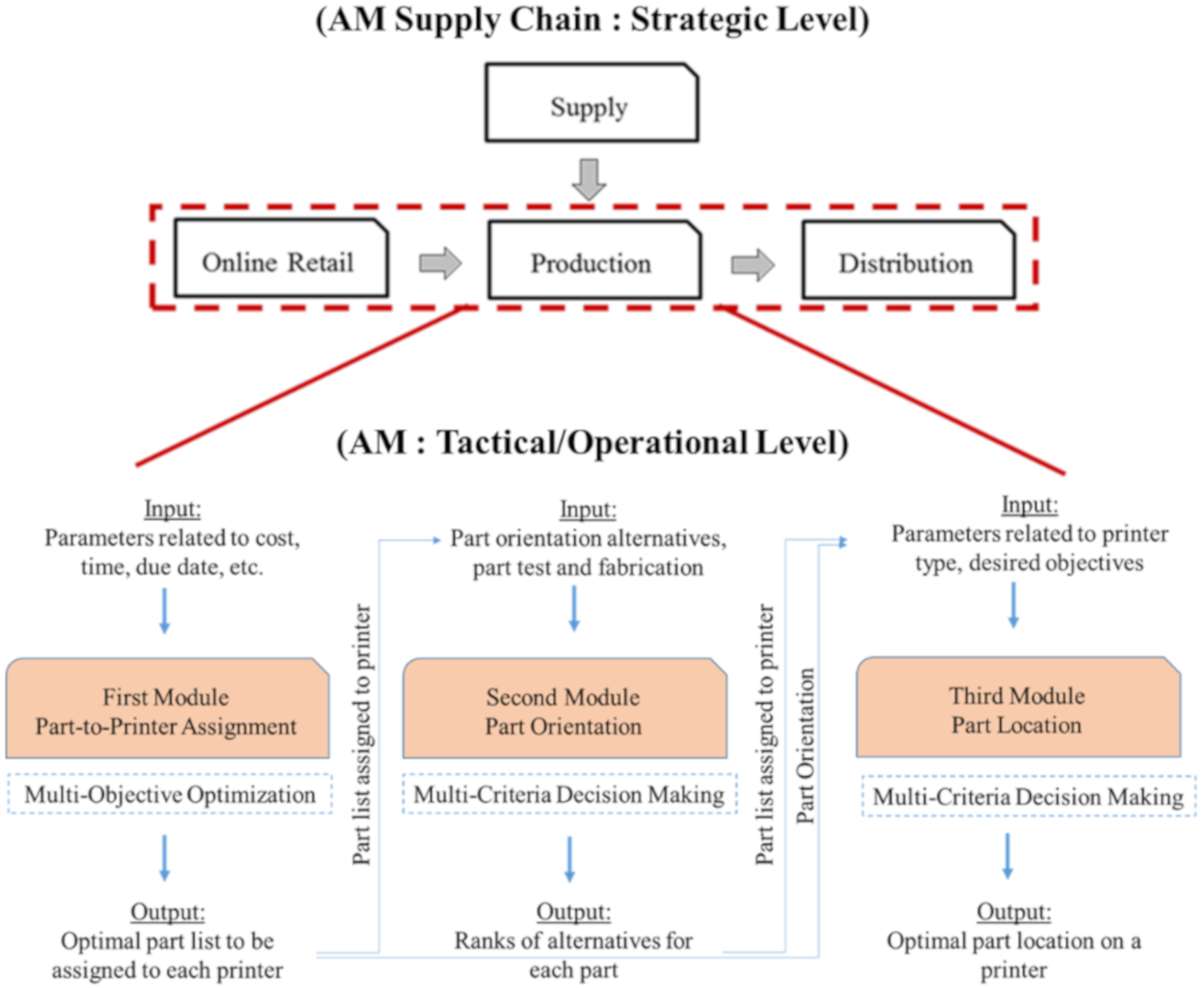
• Existing models generally considered problems at either the production or distribution planning level; the lack of integration between these two problems likely causes sub-optimality for the planners. As such, this work aimed to account for production and distribution planning.
• Process planning in AM involves various stakeholders with often conflicting requirements involving trade-offs. Thus, an AHP approach was introduced as the tool used to assess the decision analysis under multiple criteria to analyze decision-makers’ preferences under the diverse objectives of the multi-objective optimization model.
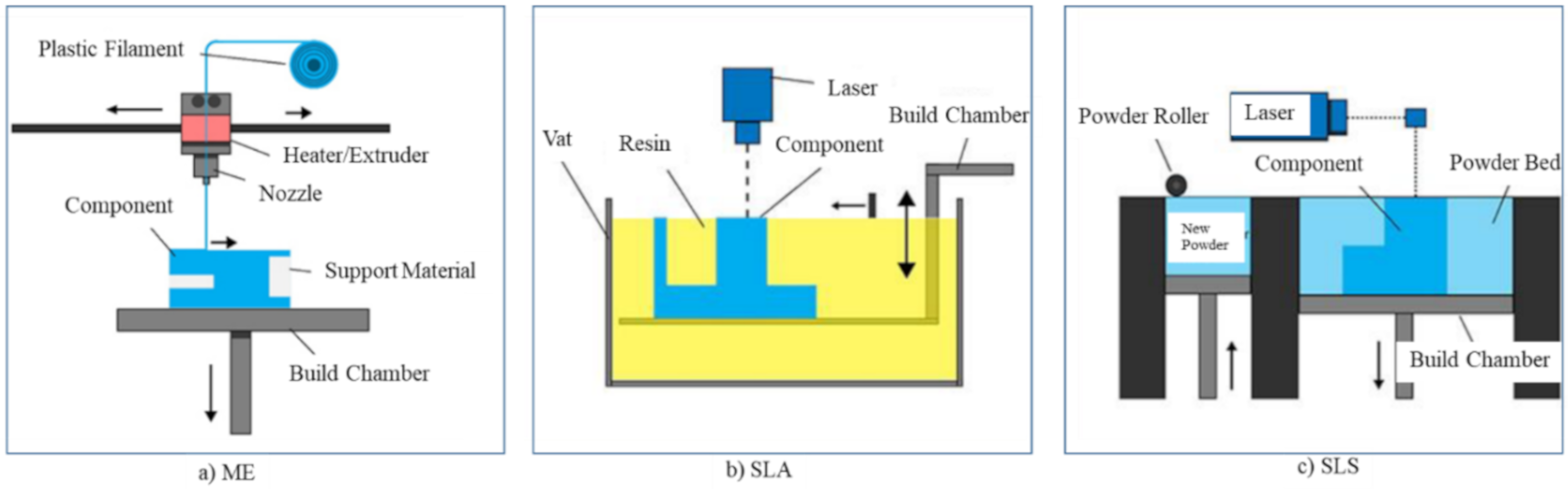
• Rather than investigating a singular AM technology as prior researchers have tended to do, three AM technologies (i.e., ME, SLA, and SLS technologies) were combined and analyzed to review various aspects of AM; in addition, a case study was used to verify and validate the model. In particular, the energy source used and the part nesting or stacking capability of the build chamber were analyzed.
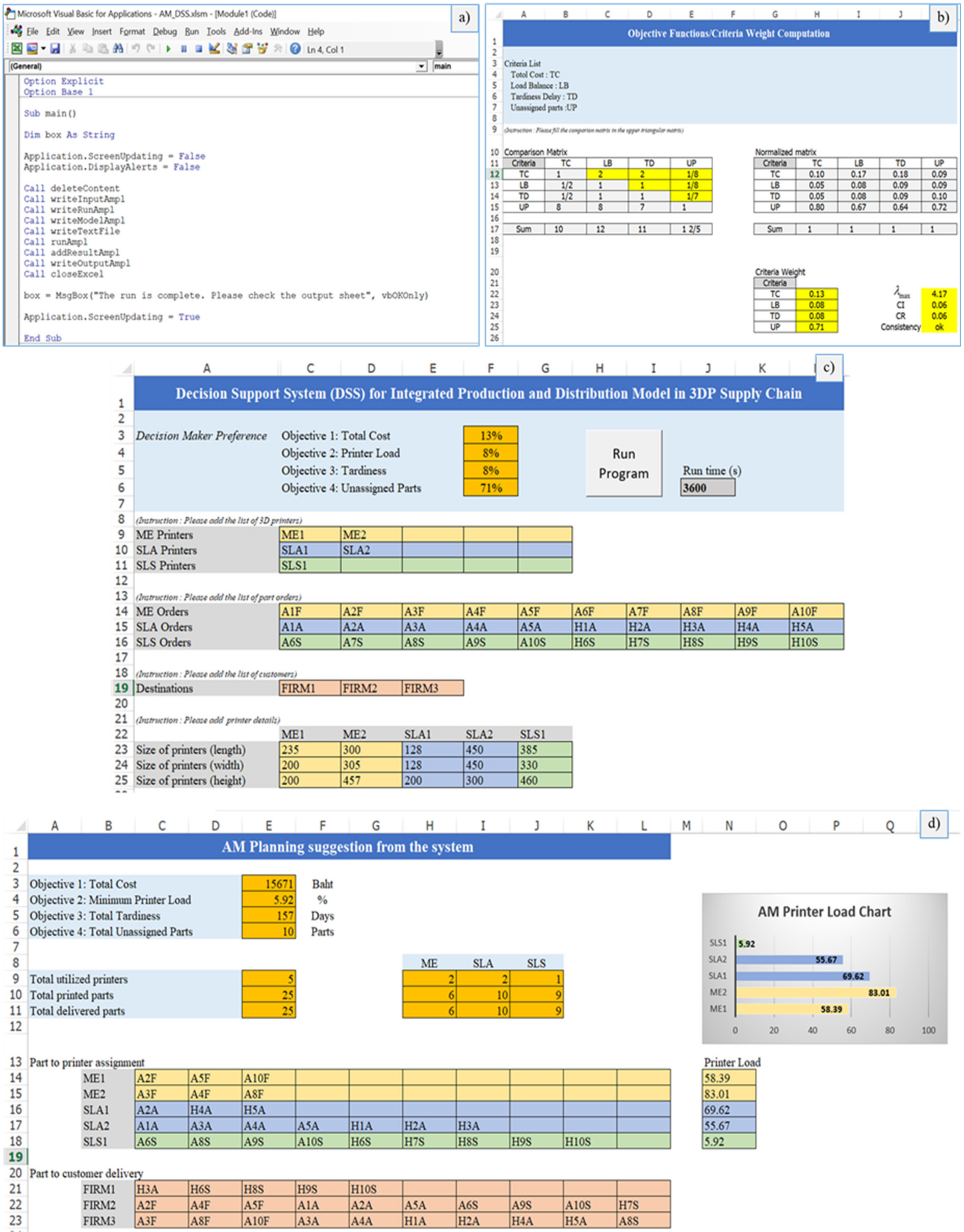
• Although AM planning-related mathematical models were recently proposed in the literature, these models lack integration with the DSS, which prohibits decision-makers that are not familiar with the mathematical notations to properly plan for their actual process. Thus, a decision-support tool was developed here to aid AM practitioners.

3. Multi-Objective Optimization Model

3.1. Problem Statement

A list of orientated parts and their associated locations on printers were taken as the input set for the mathematical model, which then analyzes how parts can be optimally scheduled to each AM printer type based on various requirements and performance measures. A decision-maker may wait for more parts for a batch or decide to print parts on a 3D printer, given the planning objectives and employed strategy. In addition, a deviation from the customers’ delivery date can be obtained, such that tardiness (delay) and earliness are computed in terms of positive and negative lateness, respectively. We next discuss the formulation of the mathematical approximations of two key technical requirements of ME, SLA, and SLS technologies, as shown in

Table 1. AM printing time and part nesting approximation.

AM Process Type	Printing Time Approximation Based on Energy Source		Part Stacking Requirement in a Build Chamber
	Laser	Extruder	With Nesting	Without Nesting
Material extrusion (ME)		√		√
Stereolithography (SLA)	√			√
Selective laser sintering (SLS)	√		√

: (1) the printing time approximation and (2) the part nesting and stacking requirement. These requirements can then be adjusted accordingly to model other AM technologies and processes.

3.1.1. Printer Time

The power source used in ME technology differs from that of SLS and SLA technologies. SLS technology uses a laser as the power source to sinter powdered material to create a 3D solid structure. Similarly, SLA uses a UV laser to selectively cure a vat of photopolymer resin layer-by-layer until the resin is solidified to form the desired 3D object. Each part scheduled to either an SLS or SLA printer will be scanned by a laser layer-by-layer at approximately the same time. Conversely, ME technology produces a part by extruding a small filament of molten material from a heated nozzle to form layers of parts. Thus, each layer of each part scheduled to an ME printer is dependent on the tool-path of the extruder controlled by a software package.

3.1.2. Part Nesting/Stacking

The build chamber use of a particular AM technology was then accounted for. Whereas printing parts using ME and SLA printers generally require special support structures to fabricate overhanging designs, a part constructed in an SLS printer is surrounded by unsintered powder in the build chamber at all times. ME printers also demonstrate some restrictions on the slope of the overhang, whereas SLA printers use supporting structures attached to the build platform to hold newly created sections during the printing and to hold cross-sections in place. Thus, the unused area of the build chamber in the X-Y directions was instead used as a setting capacity to place multiple parts in either ME or SLA. Conversely, the SLS platform allows for part nesting using the supporting powder; thus, the volume of the build chamber in the X, Y, and Z directions was used for positioning multiple parts and thus increasing the build capacity.

3.2. Assumptions

• The printer type required for the parts ordered from customers is known. That is, the customer discusses with the manufacturer and decides beforehand which technology to use for printing. In addition, the manufacturer and customers have agreed on the properties and tolerances of the printed parts on each printer, the material desired for each specific part, and the due date to receive the printed parts.
• In this study, all assigned parts were assumed to be taken out from a printer at the same time to properly associate the time-related parameters for parts to the due date of consumers. In addition, as the total printing time for SLS and SLA depends on the layout in a batch and scanned laser technology, the scanning time for a layer is likely much less than recoating time (z-directional moving) for the printing process. Thus, to simplify the mathematical model, the print time for SLS and SLA technologies was approximated and assumed based on the maximum time of all parts, which are less than the print time for all parts. On the other hand, the print time for ME was approximated and assumed from the print time for all parts.
• Although the SLS printers sometimes need a support structure to avoid deformation from residual stress depending on the specific material used, such as metals, we assumed in this study that the manufacturer can use a surrounding powder in a build chamber to allow part nesting and to use the maximum efficiency of a printer, which is possible for some materials, such as Polyamide. On the other hand, parts to be printed do not stack on top of each other for the ME and SLA printers.
• The time- and cost-related parameters were also simplified and extrapolated from the Magics software version 18.03 from Materilise, Belgium [38] and existing literature (e.g., see [34]) to reduce the complexity of the developed model. For example, the printer cost in this study was approximated from the indirect cost involving the technician, overhead, and machine costs. The part times and costs were directly obtained from an estimate from the Magics software. The part costs, in particular, were approximated from the consumed material for each part, support (if needed), and associated waste; meanwhile, the part print time was inclusive of the printer preparation time, cooling time, and post-processing time.

3.3. Model Notation

3.3.1. Sets and Indices

$I$: Ordered parts to be printed

$J$: Available 3D printers

$I^{ME},I^{SLA},I^{SLS}$: ME parts, SLA parts, SLS parts $\subseteq I$

$J^{ME},J^{SLA},J^{SLS}$: ME printers, SLA printers, SLS printers $\subseteq J$

$K$: Destinations

3.3.2. Parameters

Part-related parameters

$c_i^{part}$: Printing cost of a part $i\in I$ ($/part)

$c_i^{holding}$: Holding cost of a remaining part $i\in I$ ($/part)

$l_i$: Projection length of a part $i\in I$ (millimeter/part)

$w_i$: Projection width of a part $i\in I$ (millimeter/part)

$h_i$: Projection height of a part $i\in I$ (millimeter/part)

$a_i$: Projection area of a part $i\in I$ (millimeter²/part)

$v_i^{convex\_hull}$: Volume of the bounding box of a part $i\in I$ (millimeter³/part)

$f^{num\_part}$: Minimum required number of parts to be assigned to operate a 3D printer

Printer-related parameters

$c_j^{printer}$: Printer cost for a printer $j\in J$ ($/printer)

$l_j^{cap}$: Build chamber length of a printer $j\in J$ (millimeter/printer)

$w_j^{cap}$: Build chamber width of a printer $j\in J$ (millimeter/printer)

$h_j^{cap}$: Build chamber height of a printer $j\in J$ (millimeter/printer)

$a_j^{cap\_max}$: Area capacity for a printer $j\in J^{ME};J^{SLA}$ (millimeter²/printer)

$v_j^{cap\_max}$: Volume capacity for a printer $j\in J^{SLS}$ (millimeter³/printer)

$b^{prod}$: Total planned production budget ($)

Distribution-related parameters

$c^{trans}$: Cost of distributing a printed part ($)

$d_k^{trans}$: Transportation distance to each destination $k\in K$ (kilometer)

$d_k$: Demand/order of each destination $k\in K$ (parts)

$u_k^{lim}$: Volume limit of the shipping capacity to each destination $k\in K$ (millimeter³)

$b^{trans}$: Total planned transportation budget ($)

Time-related parameters

$t_i^{part\_ini\_hour}$: Initial print time expected for an individual part $i\in I$ (hour)

$t_i^{late}$: Lateness computed from a deviation from the due date for a part $i\in I$ (day)

$o^{labor}$: Labor working time (hour/day)

3.3.3. Decision Variables

$X_{i,j}$: Part $i\in I$ to be scheduled to a printer $j\in J$

$Y_j$: Printer $j\in J$ scheduled for printing during a planning period

$G_{i,k}$: Printed part $i\in I$ to be shipped to destination $k\in K$

$G_k^{trans}$: Total transported parts for each destination $k\in K$

$R_i^{prod}$: Part $i\in I$ that is not scheduled for printing in a planning period

$R_k^{trans}$: Printed part that is not delivered to a destination $k\in K$

$T_i$: Positive lateness of a part $i\in I$ (day)

$B_j$: Percentage of printer area/volume that is utilized $j\in J$

3.3.4. Other Time-Related Variables

$t_i^{part\_wait\_day}$: Wait time for a part that is not scheduled for printing $i\in I$ (day/part)

$t_i^{part\_out\_day}$: Finishing time for a part that is printed $i\in I$ (day/part)

$t_i^{process\_day}$: Processing time for a part $i\in I$ (day/part)

$t_j^{printer\_hour}$: Total print time for a specific 3D printer $j\in J$ (hour/printer)

$t_j^{printer\_day}$: Total print time for a specific 3D printer $j\in J$ (day/printer)

3.4. Multi-Objective Optimization Model

3.4.1. Multi-Objective Function

The optimization model was formulated using a mixed integer-linear programming (MILP) approach with multiple objectives, as shown in (1)–(6). Objective function $Z_1$, shown in (1), minimizes the total cost, including production and transportation costs. Objective function $Z_2$, shown in (2), maximizes the minimum of the load balance for all printers regardless of the AM technologies used in the production process to reflect an efficient performance with a focus on resources. Since ME and SLA processes need support materials, assigned parts are not stacked in the Z-direction, as indicated in (3). Conversely, SLS uses unsintered materials as supports; thus, parts can be stacked in the build chamber (4). In addition, objective functions $Z_3$ and $Z_4$ (i.e., (5) and (6), respectively) are used to minimize the total lateness, as well as the total number of unprinted parts and undelivered printed parts to reflect the effective performance, focusing on the result.

$$\begin{gathered} \mathrm{Minimize} \\ {Z}_1:{\displaystyle \sum }_{j\in J}{c}_j^{pr\mathrm{int}er}{Y}_j+{\displaystyle \sum }_{i\in I}{\displaystyle \sum }_{j\in J}{c}_i^{part}{X}_{i,j}+{\displaystyle \sum }_{i\in I}{c}_i^{holding}{R}_i^{prod}+{\displaystyle \sum }_{k\in K}{c}_{}^{trans}{d}_k^{trans}{G}_k^{trans} \end{gathered}$$

(1)

$$\mathrm{Maximize}{Z}_2:{\displaystyle \sum }_{j\in J}{B}_j$$

(2)

$$B_j\le \left({\displaystyle \sum }_{i\in I^{FDM};I^{SLA}}\frac{a_i{X}_{i,j}}{a_j^{cap\_\max }}\right)\times 100;\forall j\in J^{FDM};J^{SLA}$$

(3)

$$B_j\le \left({\displaystyle \sum }_{i\in I^{SLS}}\frac{v_i^{convex\_hull}{X}_{i,j}}{v_j^{cap\_\max }}\right)\times 100;\forall j\in J^{SLS}$$

(4)

$$\mathrm{Minimize}{Z}_3:{\displaystyle \sum }_{i\in I}{T}_i$$

(5)

$$\mathrm{Minimize}{Z}_4:{\displaystyle \sum }_{i\in I}{R}_i{}^{prod}+{\displaystyle \sum }_{k\in K}{R}_k{}^{trans}$$

(6)

3.4.2. Constraint Sets

Each assigned and unassigned part is to be printed using a specific AM technology that was decided upon in the customer’s order. That is, each part is scheduled to at most one printer, depending on the requested printer (7); unassigned parts remain on the future scheduling list (8). The number of parts to be scheduled for printing must be larger than a requirement designated by a planner (9).

$${\displaystyle \sum }_{j\in J}{X}_{i,j}\le 1;\forall i\in I$$

(7)

$$R_i^{prod}=1-{\displaystyle \sum }_{j\in J}{X}_{i,j};\forall i\in I$$

(8)

$${\displaystyle \sum }_{i\in I}{\displaystyle \sum }_{j\in J}{X}_{i,j}\ge f^{num\_part}\left({\displaystyle \sum }_{i\in I}{\displaystyle \sum }_{j\in J}{X}_{i,j}+{\displaystyle \sum }_{i\in I}{R}_i^{prod}\right)$$

(9)

Parts printed using ME- and SLA-type printers must not stack on top of each other in the Z-direction since the extruded filament and photopolymer resin are used as materials in ME and SLA, respectively. In addition, these printers also require a support structure. Thus, the area of each part is used to measure the printer capacity (10). The maximum capacity of each printer is then computed with (11). In addition, the total area of all parts to be scheduled for printing on the ME and SLA printers cannot be higher than the maximum capacity restriction (12) of a printer.

$$a_i=l_i{w}_i;\forall i\in I^{FDM};I^{SLA}$$

(10)

$$a_j^{cap\_\max }=l_j^{cap}{w}_j^{cap};\forall j\in J^{FDM};J^{SLA}$$

(11)

$${\displaystyle \sum _{i\in I^{FDM};I^{SLA}}{a}_i{X}_{i,j}}\le a_j^{cap\_\max }{Y}_j;\forall j\in J^{FDM};J^{SLA}$$

(12)

Conversely, parts can be stacked and nested in the build chamber of SLS printers since the powder material is kept full and support structures are not required. Thus, the volume of each part is computed based on a bounding box (13). The maximum volume limit of each SLS printer is then computed using (14) based on the printer capacity. Additionally, the total volume of all printed parts cannot violate the maximum capacity (15) of each printer.

$$v_i=l_i{w}_i{h}_i;\forall i\in I^{SLS}$$

(13)

$$v_j^{cap\_\max }=l_j^{cap}{w}_j^{cap}{h}_j^{cap};\forall j\in J^{SLS}$$

(14)

$${\displaystyle \sum _{i\in I^{SLS}}{v}_i{X}_{i,j,k}}\le v_j^{cap\_\max }{Y}_j;\forall j\in J^{SLS}$$

(15)

In addition, sets of constraints are required to reveal the restrictions on the length, width, and height of each part. In particular, the size of each scheduled part cannot exceed the size limit of the printer (16)–(21). Here, the binary variable $U$ and an arbitrarily large number $m$ are used to restrict a part that exceeds the size of the printer’s build chamber.

$$l_i{U}_{i,j}^l\le l_j^{cap};\forall i\in I,j\in J$$

(16)

$$X_{i,j}\le U_{i,j}^{l}m;\forall i\in I,j\in J$$

(17)

$$w_i{U}_{i,j}^w\le w_j^{cap};\forall i\in I,j\in J$$

(18)

$$X_{i,j}\le U_{i,j}^{w}m;\forall i\in I,j\in J$$

(19)

$$h_i{U}_{i,j}^h\le h_j^{cap};\forall i\in I,j\in J$$

(20)

$$X_{i,j}\le U_{i,j}^{h}m;\forall i\in I,j\in J$$

(21)

The restriction for the planned production budget, inclusive of the cost of the printer, part printing, and related holding costs, is illustrated in (22).

$$\left({\displaystyle \sum }_{j\in J}{c}_j^{pr\mathrm{int}er}{Y}_j\right)+\left({\displaystyle \sum }_{i\in I}{\displaystyle \sum }_{j\in J}{c}_i^{part}{X}_{i,j}\right)+\left({\displaystyle \sum }_{i\in I}{c}_i^{holding}{R}_i^{prod}\right)\le b^{prod}$$

(22)

As the sizes and geometries of parts are varied and must be printed layer-by-layer, the print time varies by part and by AM technology. The ME technology uses a heated extruder to dispense a filament material from an extruder layer-by-layer and part-by-part; thus, the total print time for an ME printer can be computed based on the sum of the print times of all the assigned parts, as shown in (23). Conversely, SLS and SLA use laser technology, which scans each layer of all scheduled parts such that the powdered material in SLS is sintered and the photopolymer resin in SLA is cured approximately at the same time. As a result, the print time can be computed using the maximum print time based on all parts assigned to the printer since the assigned part with the greatest time requirement will determine the print time (24). This non-linear term was linearly transformed using (25)–(27), in which the auxiliary variable $S_{i,j}$ is used in the transformation process. Next, the print time in days is computed based on the print time in hours and labor working time (28).

$$t_j^{pr\mathrm{int}er\_hour}={\displaystyle \sum }_{i\in I^{FDM}}{t}_i^{part\_ini\_hour}{X}_{i,j};\forall j\in J^{FDM}$$

(23)

$$t_j^{pr\mathrm{int}er\_hour}=\max (t_{i\in I^{SLA};I^{SLS}}^{part\_ini\_hour}{X}_{i,j});\forall j\in J^{SLA};J^{SLS}$$

(24)

$$t_i^{part\_ini\_hour}{X}_{i,j}\le t_j^{pr\mathrm{int}er\_hour};\forall i\in I^{SLA};I^{SLS};\forall j\in J^{SLA};J^{SLS}$$

(25)

$$t_i^{part\_ini\_hour}{X}_{i,j}\ge t_j^{pr\mathrm{int}er\_hour}-\left(1-S_{i,j}\right)m;\forall i\in I^{SLA};I^{SLS};\forall j\in J^{SLA};J^{SLS}$$

(26)

$${\displaystyle \sum }_{i\in I^{SLA};I^{SLS}}{S}_{i,j}\ge 1;\forall j\in J^{SLA};J^{SLS}$$

(27)

$$t_j^{pr\mathrm{int}er\_day}=t_j^{pr\mathrm{int}er\_hour}/o^{labor};\forall j\in J$$

(28)

The actual time in days for each scheduled part is computed using (29), given that all parts are taken out of a printer at the same time. This non-linear term represented by the variable $W_{i,j}$ in (30) is linearly transformed using (31)–(35), in which $p$ and $q$ are arbitrary numbers.

$$t_i^{part\_out\_day}={\displaystyle \sum }_{j\in J}{t}_j^{pr\mathrm{int}er\_day}{X}_{i,j};\forall i\in I$$

(29)

$$W_{i,j}=t_j^{pr\mathrm{int}er\_day}{X}_{i,j};\forall i\in I,j\in J$$

(30)

$$t_i^{part\_out\_day}={\displaystyle \sum }_{j\in J}{W}_{i,j};\forall i\in I$$

(31)

$$W_{i,j}\le q{X}_{i,j};\forall i\in I,j\in J$$

(32)

$$W_{i,j}\ge p{X}_{i,j};\forall i\in I,j\in J$$

(33)

$$W_{i,j}\le t_j^{pr\mathrm{int}er\_day}-p\left(1-X_{i,j}\right);\forall i\in I,j\in J$$

(34)

$$W_{i,j}\ge t_j^{pr\mathrm{int}er\_day}-q\left(1-X_{i,j}\right);\forall i\in I,j\in J$$

(35)

Next, any parts that are not assigned to a printer will be assigned during the next decision-making period (36), which is the next scheduling period. The actual process time in days for all parts is computed using the constraint set (37) based on the assigned and unassigned parts. Positive lateness is then computed using (38).

$$t_i^{part\_wait\_day}=e{R}_i^{prod};\forall i\in I$$

(36)

$$t_i^{process\_day}=t_i^{part\_out\_day}+t_i^{part\_wait\_day};\forall i\in I$$

(37)

$$t_i^{late}+t_i^{process\_day}=T_i;\forall i\in I$$

(38)

We next discuss the transportation-related constraints. Initially, each printed part will be transported to a specific customer location (39). The total number of distributed parts may not meet the demand requirement at each destination; parts that are printed but not delivered in the current planning period are computed using (40) and (41). The total volume of all shipments for 3D printed parts, regardless of the printer types used, cannot exceed the shipping capacity (42). Additionally, the sum of transportation expenses, based on the distance to the destination, cannot exceed the budget (43).

$${\displaystyle \sum }_{j\in J}{X}_{i,j}={\displaystyle \sum }_{k\in K}{G}_{i,k};\forall i\in I$$

(39)

$${\displaystyle \sum }_{k\in K}{G}_{i,k}=G_K^{trans};\forall k\in K$$

(40)

$$G_K^{trans}+R_K^{trans}=d_k;\forall k\in K$$

(41)

$${\displaystyle \sum }_{i\in I}{v}_i^{convex\_hull}{G}_{i,k}\le u_k^{lim};\forall k\in K$$

(42)

$${\displaystyle \sum }_{k\in K}{c}_{}^{trans}{d}_k^{trans}{G}_k^{trans}\le b^{trans}$$

(43)

Finally, the constraints for variable dimensions are shown in (44)–(57).

$$X_{i,j}=\left\{0,1\right\};\forall i\in I,j\in J$$

(44)

$$Y_j=\left\{0,1\right\};\forall j\in J$$

(45)

$$G_{i,k}=\left\{0,1\right\};\forall i\in I;k\in K$$

(46)

$$X_{}^{prod}\ge 0$$

(47)

$$G_k^{trans}\ge 0;\forall k\in K$$

(48)

$$R_i^{prod}=\left\{0,1\right\};\forall i\in I$$

(49)

$$R_k^{trans}\ge 0;\forall k\in K$$

(50)

$$T_i\ge 0;\forall i\in I$$

(51)

$$S_{i,j}=\left\{0,1\right\};\forall i\in I^{SLA};I^{SLS};\forall j\in J^{SLA};J^{SLS}$$

(52)

$$B_j\ge 0$$

(53)

$$W_{i,j}\ge 0;\forall i\in I,j\in J$$

(54)

$$U_{i,j,}^l=\left\{0,1\right\};\forall i\in I,j\in J$$

(55)

$$U_{i,j,}^w=\left\{0,1\right\};\forall i\in I,j\in J$$

(56)

$$U_{i,j,}^h=\left\{0,1\right\};\forall i\in I,j\in J$$

(57)

4. Multi-Objective Solution

4.1. Non-Preemptive Solution Approach

The proposed optimization model in this study considers multiple objectives. Thus, the single-objective, weighted-sum method known as a non-preemptive approach is presented to find a solution from a model with multiple objectives. That is, the ideal (I) and anti-ideal (AI) solutions are initially computed, representing the best and worst solution obtained on solving a particular objective function. Then, the linear normalization technique shown in (58) is further used to obtain comparable objectives regardless of their initial units by converting each objective function with different units of measurement to be in the range [0,1]. Here, whereas $Z_i^I$ indicates the ideal solution based on the max $Z_i$ for the benefit criterion and min $Z_i$ for the cost criterion, $Z_i^{AI}$ indicates the anti-ideal solution based on min $Z_i$ for the benefit criterion and max $Z_i$ for the cost criterion. Then, all the linearly normalized objective functions are transformed to a maximization problem and can be reformulated as the weighted objective model, asc presented in (59). Weight ${\alpha }_i$ emphasizes the importance of objective function $i$, which can be obtained using the AHP method presented in the next section.

$$0\le \frac{Z_i-Z_i^{AI}}{Z_i^I-Z_i^{AI}}\le 1\mathrm{for}\mathrm{benefit}\mathrm{criterion};0\le \frac{Z_i^{AI}-Z_i}{Z_i^{AI}-Z_i^I}\le 1\mathrm{for}\cos \mathrm{t}\mathrm{criterion}$$

(58)

$$\mathrm{Maximize}{\alpha }_1\left(\frac{Z_1^{AI}-Z_1}{Z_1^{AI}-Z_1^I}\right)+{\alpha }_2\left(\frac{Z_2-Z_2^{AI}}{Z_2^I-Z_2^{AI}}\right)+{\alpha }_3\left(\frac{Z_3^{AI}-Z_3}{Z_3^{AI}-Z_3^I}\right)+{\alpha }_4\left(\frac{Z_4^{AI}-Z_4}{Z_4^{AI}-Z_4^I}\right)$$

(59)

4.2. Analytic Hierarchy Process (AHP)-Based Criteria Weights

This section discusses how the weight parameters (${\alpha }_i$) are obtained from a decision-maker. Vaidya and Kumar [39] indicated that future applications of AHP include decision-making and other complex issues involving an integrated application of AHP and other techniques. More details regarding recent AHP-based techniques and applications can be found in the literature (e.g., [40,41,42]). AHP works by transforming empirical comparisons into numerical values, allowing a decision-maker to incorporate their experience and judgment into an evaluation. In this study, the relative importance scale of 1–9 was used for pairwise comparisons, where indifference corresponds to 1; weak preference to 3; definite preference to 5; strong preference to 7; very strong preference to 9; and 2, 4, 6, and 8 are used as intermediate values for comparisons. These pairwise comparisons are then recorded in a matrix, as shown in (60). The diagonal elements are always 1, illustrating the comparisons of the same element. Only the upper triangular matrix needs to be evaluated, as the reciprocal value in the lower triangular matrix can be simply converted. Thus, there are $\left[n\times \left(n-1\right)\right]/2$ judgments required to solve the matrix, where $n$ is the number of evaluated criteria.

$$A=\left[\begin{array}{cccc}1& a_{12}& \dots & a_{1n}\\ a_{21}& 1& \dots & a_{2n}\\ \dots & a_{ji}=\raisebox{1ex}{$1$}\!\left/ \!\raisebox{-1ex}{$a_{ij}$}\right.& 1& \dots \\ a_{n1}& \dots & \dots & 1\end{array}\right]$$

(60)

where $a_{ij}$ is the comparison between i and j based on the importance scale.

Once the comparison matrix is normalized by dividing each value by the total value in each column, the normalized principal eigenvector is calculated, which provides the criteria weights by computing the row average. To ensure that a decision-maker has been consistent, the consistency index (CI) (61) and consistency ratio (CR) (62) can be calculated, based on the maximum eigenvalue (${\lambda }_{\max }$) and random consistency index (RI), respectively. The RI values can be obtained based on the following (n, RI) pairs: (1, 0.00), (2, 0.00), (3, 0.58), (4, 0.90), (5, 1.12), (6, 1.24), (7, 1.32), (8, 1.41), (9, 1.45), and (10, 1.49). The CR value is used to interpret the consistency, in which a CR of less than 10% implies an acceptable consistency.

$$CI=\frac{{\lambda }_{\max }-n}{n-1}$$

(61)

$$CR=\frac{CI}{RI}$$

(62)

Following the AHP approach, the objective functions and criteria weight were computed, as shown in

Table 2. Pairwise comparison matrix and criteria weight based on the analytic hierarchy process (AHP) approach.

Criteria	Total Cost	Load Balance	Total Lateness	Unassigned Parts	Criteria Weight
Total cost	1 (0.100)	2 (0.167)	2 (0.182)	1/8 (0.090)	0.135
Load balance	1/2 (0.050)	1 (0.083)	1 (0.091)	1/8 (0.090)	0.078
Total lateness	1/2 (0.050)	1 (0.083)	1 (0.091)	1/7 (0.103)	0.082
Unassigned parts	8 (0.800)	8 (0.667)	7 (0.636)	1 (0.718)	0.705

Note: Parenthetical values denote normalized values.

. Initially, an AM expert rated the criteria preference using the AHP’s scale for all pairwise comparisons. For example, the total cost criterion was indifferent to weakly preferred (i.e., 2) for both the load balance and total lateness criteria, whereas the total unassigned parts criterion was strongly to very strongly preferred to the total cost criterion (i.e., 1/8). The pairwise-comparison matrix was then normalized, the eigenvector was calculated, the maximum eigenvector (${\lambda }_{\max }$) was obtained, and the CI and CR were computed: ${\lambda }_{\max }$ = 4.17, CI = (4.17 − 4)/(4 − 1) = 0.06. An RI of 0.90 was then chosen; as such, CR = 0.06/0.90 = 0.06 or 6%. Since the value of CR was less than 10% (i.e., 0.1), the judgments were found to be acceptably consistent. The obtained criteria weights for the total cost ($Z_1$), load balance ($Z_2$), total lateness ($Z_3$), and total unassigned parts ($Z_4$) were thus 0.135, 0.078, 0.082, and 0.705, respectively (Table 2). That is, the criteria were ranked from most to least important as total unassigned parts, total cost, total lateness, and load balance, respectively. These obtained criteria weights were then used in the non-preemptive method introduced earlier.

5. Case Study and Discussion

The case study and designed experiment are discussed in this section. The mathematical model was developed and analyzed using A Mathematical Programming Language (AMPL) software with CPLEX solver version 12.10 from AMPL Optimization Inc., CA, USA [43]. In particular, CPLEX solves integer-type problems by using algorithms inclusive of branch-and-bound, cut generators, and heuristics. The case study and data for an experimental design were analyzed on a PC with the following properties: an Intel (R) Core (TM) i7-7500 CPU, 2.70 GHz, and 16.0 GB of RAM.

5.1. Case Study Data

A 3DP dataset related to automotive and healthcare components was applied to test the model functionality, as shown in

Table 3. Case study parts.

Automotive (A) *					Healthcare (H) **
CAD File	Length (mm)	Width (mm)	Height (mm)	Volume/ Proj. Area	CAD File	Length (mm)	Width (mm)	Height (mm)	Volume/ Proj. Area
1	214	120	7	179,760/ 25,680	1	129	140	230	4,153,800/ 18,060
2	78	77	45	270,270/ 6006	2	100	84	118	991,200/ 8400
3	291	85	88	2,176,680/ 24,735	3	50	79	27	106,650/ 3950
4	125	283	26	919,750/ 35,375	4	50	48	29	69,600/ 2400
5	72	24	28	48,384/ 1728	5	30	100	56	168,000/ 3000
6	311	48	44	656,832/ 14,928	6	43	53	39	88,881/ 2279
7	185	353	11	718,355/ 65,305	7	27	38	25	25,650/ 1026
8	176	90	60	950,400/ 15,840	8	51	102	35	950,400/ 15,840
9	89	80	52	370,240/ 7120	9	83	68	86	485,384/ 5644
10	135	146	33	650,430/ 19,710	10	85	84	7	49,980/ 7140

Remark: * Data adapted from Ransikarbum et al. [11]. ** Data adapted from NIH 3D Print Exchange [44]. CAD: Computer-aided design.

. Thirty parts were planned and scheduled for printing, including 10 automotive parts requiring ME (parts A1–A10), 5 automotive and 5 healthcare parts requiring SLA (parts A1–A5 and H1–H5), and 5 automotive and 5 healthcare parts requiring SLS (parts A6–A10 and H6–H10). In addition, three shipping destinations with varied transportation requirements were included. Five printers were assumed available in this study: two ME printers (Sprout with a 235 × 200 × 200 mm build chamber and MakerBot Z18 with a 300 × 305 × 457 mm build chamber), two SLA printers (Formlabs with a build chamber of 128 × 128 × 200 mm and Replas RPS with a build chamber of 450 × 450 × 300 mm), and one SLS printer (sPro 60 from 3D Systems with a 385 × 330 × 460 mm build chamber). Then, part-related parameter data were obtained from Magics [38] and by randomly generating data, as illustrated in

Table 4. Parameters for the case study and experimental design.

Parameters	Details
Cost-Related Parameters
Printer cost ($)	ME (Small 500, Large 800); SLA (Small 600, Large 1000); SLS (Small 1200, Large 1500)
Part cost ($)	Magics; ME: Uniform (20, 100); SLA: Uniform (50, 200); SLS: Uniform (100, 300)
Part-holding cost ($)	ME: Uniform (20, 100); SLA: Uniform (50, 200); SLS: Uniform (100, 300)
Transportation cost ($)	Uniform (5, 10)
Production budget ($)	20,000 a
Transportation budget ($)	20,000 a
Part and Printer-Related Parameters
Projection length/width/height (mm.)	ME: Uniform (80, 220); SLA: Uniform (90, 230); SLS: Uniform (100, 250)
Shrink-wrap and bounding box volume (mm.)	Magics
Printer capacity (mm.)	ME (Small 235 × 200 × 200, Large 300 × 305 × 457); SLA (Small 128 × 128 × 200, Large 450 × 450 × 300); SLS (Small 385 × 330 × 460, Large 700 × 380 × 580)
Fraction determining the minimum area/volume of a printer	3% a
Fraction determining the minimum number of parts required to operate a printer	20% a
Logistics-Related Parameters
Transportation distance (km.)	Uniform (50, 100)
Demand and order (pieces)	Uniform (5, 30)
Shipping capacity (m3)	Uniform (5, 8)
Time-Related Parameters
Print time for an individual part (hours)	Magics ME: Uniform (5, 30); SLA: Uniform (10, 35); SLS: Uniform (3, 20)
Labor working hours	8 h/day
Lateness computed from the customers’ due dates (days)	U (−5, 5)
Wait time for the next period for parts that are not assigned (days)	7 days

^a: The parameter value was adjusted according to the number of parts and printers.

. Furthermore, there are also existing cost and time models in the literature (e.g., see [34]).

5.2. Multi-Objective Solution

The case study was initially solved using the weighted-sum objective model, as presented in

Table 5. Results of the case study based on each objective function.

Desired Criteria	Z1	Z2	Z3	Z4	Multi-Objective
Solve time (s)	0.141	0.062	0.547	0.062	0.453
Assigned printers	ME1 SLA1 SLS1	ME1, ME2 SLA1, SLA2 SLS1	ME1, ME2 SLA1, SLA2 SLS1	ME1, ME2 SLA2 SLS1	ME1, ME2 SLA1, SLA2 SLS1
Assigned parts	ME1 (A2, 5, 10) SLA1 (H3, 4) SLS1 (A8, 10; H8)	ME1 (A2, 5, 10) ME2 (A3, 4, 8) SLA1 (A2; H3, 5) SLA2 (A1, 3, 4; H1, 2, 4) SLS1 (A6, 8, 9, 10; H6, 7, 8, 9, 10)	ME1 (A2, 5, 10) ME2 (A3, 4, 8) SLA1 (A5; H4, 5) SLA2 (A1, 4, 5; H1, 2, 3) SLS1 (A6, 8, 9; H6, 8, 9, 10)	ME1 (A2, 5, 10 )ME2 (A3, 4, 8) SLA2 (A1, 2, 3, 4, 5; H1, 2, 3, 4, 5) SLS1 (A6, 8, 9, 10; H6, 7, 8, 9, 10)	ME1 (A2, 5, 10) ME2 (A3, 4, 8) SLA1 (A2; H4, 5) SLA2 (A1, 4, 5; H1, 2, 3) SLS1 (A6, 8, 9, 10; H6, 7, 8, 9, 10)
Part shipment	Firm 2 (A2, 5, 8, 10, 10; H3, 4, 8)	Firm 1 (A2, 3, 6, 9, 10; H2, 3, 5, 7, 8) Firm 2 (A1, 3, 4, 4, 8, 10; H1, 10) Firm 3 (A2, 5, 8; H4, 6, 9)	Firm 1 (A2, 2, 4, 4, 5; H2, 4, 6, 8, 9) Firm 2 (A3, 8, 8, 9, 10; H5,) Firm 3 (A1, 5, 6; H1, 3, 10)	Firm 1 (A2, 4, 8; H6, 9, 10) Firm 2 (A1, 5, 6, 8, 9, 10, 10; H4, 5) Firm 3 (A2, 3, 3, 4, 5; H1, 2, 3, 7, 8)	Firm 1 (A2, 3, 8; H5) Firm 2 (A2, 4, 5, 6; H2, 4, 5, 7, 8, 9) Firm 3 (A1, 4, 8, 9, 10, 10; H1, 3, 6, 10)
Total operating cost ($)	6,158	15,827	15,108	15,256	14,999
Load balance	ME1 (58.39%) ME2 (0%) SLA1 (38.76%) SLS2 (0%) SLS1 (3.05%)	ME1 (58.39%) ME2 (83.01%) SLA1 (79.08%) SLA2 (54.05%) SLS1 (5.92%)	ME1 (58.39%) ME2 (83.01%) SLA1 (69.62%) SLA2 (43.45%) SLS1 (4.76%)	ME1 (58.39%) ME2 (83.01%) SLA1 (0%) SLA2 (61.30%) SLS1 (5.92%)	ME1 (58.39%) ME2 (83.01%) SLA1 (69.62%) SLA2 (43.45%) SLS1 (5.92%)
Maximin Load	0%	5.92%	4.76%	0%	5.92%
Total lateness (days)	196	622	138	415	145
Total parts unassigned (parts)	22/22 (ME: 7; SLA: 8; SLS: 7)	6/6 (ME: 4; SLA: 1; SLS: 1)	8/8 (ME: 4; SLA: 1; SLS: 3)	5/5 (ME: 4 SLA: 0 SLS: 1)	6/6 (ME: 4 SLA: 1 SLS: 1)

. The computation time was also solved in seconds since the problem size of the case study was relatively small. Each obtained objective function was then used as an ideal solution of the non-preemptive method (i.e., $Z_1^I$, $Z_2^I$, $Z_3^I$, and $Z_4^I$ were 6158, 5.92, 139, and 10, respectively). By converting the maximization to minimization and vice versa, the non-ideal solutions were obtained (i.e., $Z_1^{AI}$, $Z_2^{AI}$, $Z_3^{AI}$, and $Z_4^{AI}$ were 16,596, 0, 663, and 46, respectively). Solving each objective function alone yielded different printer schedules. The parts assigned to each printer during the production process and distributed to each location during the distribution process differed depending on the planning objectives. For example, solving Z₁ with the minimum cost policy resulted in the least usage of the smallest-sized printers (i.e., the small ME, SLA, and SLS printers) and a small number of parts assigned to meet the minimum requirements or a daily operation with the minimum possible cost. Conversely, solving Z₂ (i.e., maximizing the load balance of all printers, regardless of AM type) and Z₃ (i.e., minimizing lateness) required all existing printers to be used. Solving Z₄ (i.e., minimizing the total number of unassigned parts) required that all existing printers be used, except the small SLA printer.

The solution set of each single-objective model highlighted trade-offs among the criteria. For example, solving Z₁ yielded the lowest total operating and distribution cost (i.e., $6,158); however, the outputs related to the load balance and total lateness did not outperform solving other objective functions, and a high number of parts were left unassigned when the holding costs were considered. Meanwhile, solving Z₃ provided the least total lateness (138 days), the total operating cost was higher than that of Z₁ (i.e., $15,827 vs. $6,158), the load balance was less than that of Z₂ (i.e., 4.76% vs. 5.92%), and there were a greater number of unassigned parts than that of Z₄ (i.e., 8 vs. 5). Then, a multi-objective solution was obtained by applying a non-preemptive method. Given the ideal (I) and anti-ideal (AI) solutions obtained earlier, the developed model was converted into a single-objective weighted optimization model. For example, let us assume that a decision-maker is interested in all objectives with equal preference, implying that the criteria weights are all equal. The optimal result, which was solved within a second, shows that the model tried to balance all the criteria optimally. That is, the total cost was found to be $14,999, the load balance was found to be at least 5.92%, the total lateness was 145 days, and the total unassigned parts were 6.

5.3. Decision-Support System

In reality, a decision-maker may prefer one objective to another. The AHP method discussed earlier can be implemented to obtain criteria weights based on preferences from the decision-maker. A Visual Basic for Applications (VBA)-based interactive input–output system was developed in Microsoft Excel to aid practitioners not familiar with the mathematical notations, as shown in Figure 3. The developed model-driven DSS can be used to access and manipulate the integrative AHP and multi-objective optimization model, as well as assist decision-makers in planning the production and distribution for a network of AM printers. The embedded macro VBA coding and AHP input sheet, in which a decision-maker makes the pairwise comparisons among the criteria to obtain the criteria weights, is shown in Figure 3a,b, respectively. The AHP-based criteria weights, shown in cells H22:H25 in Figure 3b, were linked to the objective weights in cells F3:F6 in Figure 3c. The input sheet of the developed MILP, which allows a decision-maker to specify the parts to be printed and distributed, as well as the parameters related to the different requirements of the acquired AM printers, are illustrated in Figure 3c. Once “Run Program” is clicked, the underlining model analyzes the data and presents outputs, as shown in Figure 3d; the objective functions are shown in cells E3:E6. Additionally, the variables relevant to the part-to-printer assignment, part distribution, and load balance for each printer are presented.

With an emphasis on the total unassigned parts’ objective function (i.e., criteria weights were 0.13 for the total cost, 0.08 for the load balance, 0.08 for the total lateness, and 0.71 for the total unassigned parts), the total number of unassigned parts decreased when compared with the outputs from the equal-weight solution (i.e., criteria weights were 0.25 for the total cost, 0.25 for the load balance, 0.25 for the total lateness, and 0.25 for the total unassigned parts). As expected, this was due to there being trade-offs with other objective functions.

5.4. Computation Time Result

An experiment was then conducted to evaluate the model complexity by varying three key factors, which were the number of parts, printer types, and distribution locations. Matlab software version 8.5 from MathWorks, Natick, MA, USA was used to randomly generate test data by varying the random number of parts scheduled to each AM printer at two levels (i.e., 100 parts and 500 parts). We note that multiple items of the same part type or different part types in the same batch were allowed. The number of printers and size of the build chambers for ME, SLA, and SLS were tested at two levels (i.e., 5 printers and 10 printers). The number of distribution locations was also evaluated at two levels (i.e., 5 locations and 10 locations) with random distances and demands. Ten replications of data were randomly generated for each test combination, yielding a total of (2)³(10) = 80 experimental runs. The resulting average computation time is shown in

Table 6. Aggregated computation time for a designed experiment (seconds).

Factors/Levels		Z1	Z2	Z3	Z4	Multi-Objective
Printers	5	0.79	15.33	1818.22	1.24	1942.39
	10	4.01	84.88	3080.53	310.03	3420.42
Parts	100	1.08	2.60	1298.75	183.85	1782.87
	500	3.72	97.61	3600	127.43	3579.94
Destinations	5	2.52	4.28	2612.64	4.02	2644.53
	10	2.28	95.93	2286.11	307.26	2718.28
Grand average		2.40	50.11	2449.38	155.64	2681.40

, in which the computation time for each run was capped at 1 h.

The aggregated average computation time based on the varied printer, part, and destination numbers with two levels for each factor is shown in Table 6. The results show that varying the number of printers, parts, or locations affected the computation time of the model. In particular, the average computation time suggested that minimizing the total cost (i.e., solving Z₁) required the least average computation time at a few seconds (i.e., 2.40 s), whereas minimizing the total lateness or delays (i.e., solving Z₃) required the highest average computation time (i.e., 2449.38 s). Minimizing the load balance or the total number of unassigned parts not printed or delivered (i.e., solving Z₂ or Z₄) required an acceptable average computation time of a few minutes (i.e., 50.11 and 155.64 s). Regarding the computation time for the non-preemptive method of the multi-objective solution, the equal-weight consideration required a higher average computation time, regardless of the combination of factors and level of printers, parts, or destinations. This result was not surprising since solving the model with an equal-weight consideration aimed to balance all the objective functions at the same time, requiring a higher complexity and hence computation time.

6. Conclusions and Future Research

AM, also known as 3DP, became an essential method that is capable of streamlining and expediting product development, making prototypes, and fabricating tooling components and final production parts, as well as reducing the time to market, improving product quality, and reducing costs. Aspects requiring further research include process planning and supply chain design, especially printer selection, part orientation, and part-to-printer scheduling. In this study, an integrative multi-objective optimization model and AHP technique were introduced for integrated production and distribution problems in AM. The developed multi-objective optimization model reflected diverse requirements by considering the operating and distribution costs, the load balance of printers, delays, and the remaining parts not assigned and distributed. The AHP was employed to evaluate the objective weights for the non-preemptive approach of the multi-objective solution.

The developed model employed ME, SL, and SLS processes; technical aspects were evaluated for printer-time approximation and part-nesting requirements. The model was verified and validated using selected automotive and healthcare components, and the relevant data for parts, printers, and distribution locations were collected to test the model functionalities. The designed experiment for the computation time was evaluated based on three key factors: the number of parts, printers, and distribution locations, each with two levels. Two criteria weight settings, with equal-weight consideration and with the employed AHP method, were also used to analyze the model in this study. The results indicated the presence of trade-offs among conflicting criteria of the proposed model. A decision-support tool for AM planning was developed using Excel to aid practitioners not familiar with AHP mathematical notations or the optimization approach. The development of the decision-support tool is needed to reduce the gap between researchers and practitioners in AM.

This study provided a practical analysis of the integrated production and distribution problems for AM. As the AM supply chain becomes more complex and involves shared AM printers in a business platform, evaluating how a business can improve its production and process planning to improve the capacity, revenue, and management practices is important. Directions for future research should include evaluating other solution methods in the realm of metaheuristics to improve the computation time due to the NP-hard complexity of the model for practical, effective solutions. Although the illustrated case study was solved in a few seconds, a relatively low number of parts, printers, and delivery locations were included; the computation time will increase as more variables are included. Additionally, this study focused on AM; however, production facilities may aim to use both AM printers and traditional manufacturing equipment to fabricate a variety of parts. Thus, enhancing the scheduling system to incorporate both types of technologies should also be a subject of future study. Lastly, to simplify the complexity of the developed mathematical model, associated assumptions are needed. Thus, these assumptions are to be further relaxed to incorporate practical aspects of AM. For example, the scheduling criterion induced by the material variations from the manufacturers may be considered such that the number of changeovers is minimized for batch replacement. Some existing quality issues (e.g., deformation in specific material in the SLS process, printed part damage) may also be considered during the model development. That is, given a possibility that frequently obtained prints may be damaged and need to be repeated, an uncertainty aspect could be incorporated in the mathematical model using stochastic programming in the future.

References

1. Thompson, M.K.; Moroni, G.; Vaneker, T.; Fadel, G.; Campbell, R.I.; Gibson, I.; Bernard, A.; Schulz, J.; Graf, P.; Ahuja, B.; et al. Design for Additive Manufacturing: Trends, opportunities, considerations, and constraints. Cirp Ann. 2016, 65, 737–760. [Google Scholar] [CrossRef]
2. Wohlers, T. Wohlers Report 2018; Wohlers Associates, Inc.: Fort Collins, CO, USA, 2018. [Google Scholar]
3. Ha, S.; Ransikarbum, K.; Kim, N. Phenomenological deformation patterns of 3D printed products in a selective laser sintering process. In Proceedings of the 18th International Conference on Industrial Engineering, Seoul, Korea, 10–12 October 2016; pp. 10–12. [Google Scholar]
4. Ha, S.; Ransikarbum, K.; Han, H.; Kwon, D.; Kim, H.; Kim, N. A dimensional compensation algorithm for vertical bending deformation of 3D printed parts in selective laser sintering. Rapid Prototyp. J. 2018, 24, 955–963. [Google Scholar] [CrossRef]
5. Kim, N.; Bhalerao, I.; Han, D.; Yang, C.; Lee, H. Improving surface roughness of additively manufactured parts using a photopolymerization model and multi-objective particle swarm optimization. Appl. Sci. 2019, 9, 151. [Google Scholar] [CrossRef] [Green Version]
6. Ransikarbum, K.; Kim, N. Multi-criteria selection problem of part orientation in 3D fused deposition modeling based on analytic hierarchy process model: A case study. In Proceedings of the 2017 IEEE International Conference on Industrial Engineering and Engineering Management (IEEM), Singapore, 10–13 December 2017; pp. 1455–1459. [Google Scholar]
7. Ransikarbum, K.; Kim, N. Data envelopment analysis-based multi-criteria decision making for part orientation selection in fused deposition modeling. In Proceedings of the 2017 4th International Conference on Industrial Engineering and Applications (ICIEA), Nagoya, Japan, 21–23 April 2017; pp. 81–85. [Google Scholar]
8. Ransikarbum, K.; Pitakaso, R.; Kim, N. Evaluation of Assembly Part Build Orientation in Additive Manufacturing Environment using Data Envelopment Analysis. In MATEC Web of Conferences; EDP Sciences: Les Ulis, France, 2019; Volume 293, p. 02002. [Google Scholar]
9. Ransikabum, K.; Yingviwatanapong, C.; Leksomboon, R.; Wajanavisit, T.; Bijaphala, N. Additive Manufacturing-based Healthcare 3D Model for Education: Literature Review and A Feasibility Study. In Proceedings of the 2019 Research, Invention, and Innovation Congress (RI2C), Bangkok, Thailand, 11–13 December 2019; pp. 1–6. [Google Scholar]
10. Sculpteo. Comparison between 3D Printing and Traditional Manufacturing Processes for Plastics. 2018. Available online: http://www.sculpteo.com/en/3d-printing (accessed on 5 June 2018).
11. Ransikarbum, K.; Ha, S.; Ma, J.; Kim, N. Multi-objective optimization analysis for part-to-Printer assignment in a network of 3D fused deposition modeling. J. Manuf. Syst. 2017, 43, 35–46. [Google Scholar] [CrossRef]
12. Taufik, M.; Jain, P.K. Role of build orientation in layered manufacturing: A review. Int. J. Manuf. Technol. Manag. 2013, 27, 47–73. [Google Scholar] [CrossRef]
13. Canellidis, V.; Giannatsis, J.; Dedoussis, V. Genetic-algorithm-based multi-objective optimization of the build orientation in Stereolithography. Int. J. Adv. Manuf. Technol. 2009, 45, 714–730. [Google Scholar] [CrossRef]
14. Freens, J.P.; Adan, I.J.; Pogromsky, A.Y.; Ploegmakers, H. Automating the production planning of a 3D printing factory. In Proceedings of the IEEE 2015 Winter Simulation Conference (WSC), Huntington Beach, CA, USA, 6–9 December 2015; pp. 2136–2147. [Google Scholar]
15. Ransikarbum, K.; Mason, S.J. Multiple-Objective Analysis of Integrated Relief Supply and Network Restoration in Humanitarian Logistics Operations. Int. J. Prod. Res. 2016, 54, 49–68. [Google Scholar] [CrossRef]
16. Ransikarbum, K.; Mason, S.J. Goal programming-based post-disaster decision making for integrated relief distribution and network restoration. Int. J. Prod. Econ. 2016, 182, 324–341. [Google Scholar] [CrossRef]
17. Velasquez, M.; Hester, P.T. An analysis of multi-criteria decision making methods. Int. J. Oper. Res. 2013, 10, 56–66. [Google Scholar]
18. Saaty, T.L. Relative measurement and its generalization in decision making why pairwise comparisons are central in mathematics for the measurement of intangible factors—The analytical hierarchy/network process, RACSAM-Revista de la Real Academia de Ciencias Exactas, Fiscas y naturales. Series A. Mathematics 2008, 102, 251–318. [Google Scholar]
19. Saaty, T.L.; Sagir, M. Extending the measurement of tangibles to intangibles. Int. J. Inf. Technol. Decis. Mak. 2009, 8, 7–27. [Google Scholar] [CrossRef]
20. ASTM. Standard Terminology for Additive Manufacturing Technologies; ASTM International: West Conshohocken, PA, USA, 2012. [Google Scholar]
21. Bourell, D.L.; Beaman, J.J.; Leu, M.C.; Rosen, D.W. A Brief History of Additive Manufacturing and the 2009 Roadmap for Additive Manufacturing: Looking Back and Looking Ahead. In Proceedings of the RapidTech 2009: US-TURKEY Workshop on Rapid Technologies, Istanbul, Turkey, 24–25 September 2009; pp. 5–11. [Google Scholar]
22. Berman, B. 3-D printing: The new industrial revolution. Bus. Horiz. 2012, 55, 155–162. [Google Scholar] [CrossRef]
23. Gardan, J. Additive manufacturing technologies: State of the art and trends. Int. J. Prod. Res. 2016, 54, 3118–3132. [Google Scholar] [CrossRef]
24. Han, J.Y. A study on the Prototype Modeling Method using 3D Printing. J. Packag. Cult. Des. Res. 2013, 34, 97–109. [Google Scholar]
25. 3D Hubs. Available online: https://www.3dhubs.com/ (accessed on 15 January 2020).
26. Shapeways. Available online: https://www.shapeways.com/ (accessed on 15 January 2020).
27. Achillas, C.; Aidonis, D.; Iakovou, E.; Thymianidis, M.; Tzetzis, D. A methodological framework for the inclusion of modern additive manufacturing into the production portfolio of a focused factory. J. Manuf. Syst. 2015, 37, 328–339. [Google Scholar] [CrossRef]
28. Manogharan, G.; Wysk, R.A.; Harrysson, O.L.A. Additive manufacturing-integrated hybrid manufacturing and subtractive processes: Economic model and analysis. Int. J. Comput. Integr. Manuf. 2016, 29, 473–488. [Google Scholar] [CrossRef]
29. Zhang, Y.; Bernard, A.; Harik, R.; Karunakaran, K.P. Build orientation optimization for multi-part production in additive manufacturing. J. Intell. Manuf. 2017, 28, 1393–1407. [Google Scholar] [CrossRef]
30. Hasan, S.; Rennie, A.E.W. The Application of Rapid Manufacturing Technologies in the Spare Parts Industry. In Proceedings of the Solid Freeform Fabrication Symposium, Austin, TX, USA, 4–8 August 2008; pp. 584–590. [Google Scholar]
31. Holmström, J.; Partanen, J.; Tuomi, J.; Walter, M. Rapid manufacturing in the spare parts supply chain: Alternative approaches to capacity deployment. J. Manuf. Technol. Manag. 2010, 21, 687–697. [Google Scholar] [CrossRef]
32. Holmström, J.; Partanen, J. Digital manufacturing-driven transformations of service supply chains for complex products. Supply Chain Manag. Int. J. 2014, 19, 421–430. [Google Scholar] [CrossRef]
33. Khajavi, S.H.; Partanen, J.; Holmström, J. Additive manufacturing in the spare parts supply chain. Comput. Ind. 2014, 65, 50–63. [Google Scholar] [CrossRef]
34. Thomas, D.S.; Gilbert, S.W. Costs and Cost Effectiveness of Additive Manufacturing. NIST Speical Publ. 2014, 1176, 12. [Google Scholar]
35. Verma, A.; Rai, R. Energy efficient modeling and optimization of additive manufacturing processes. In Proc. of Solid Freeform Fabrication Symposium; University of Texas: Austin, TX, USA, 2013; pp. 231–241. [Google Scholar]
36. Yoon, H.S.; Lee, J.Y.; Kim, H.S.; Kim, M.S.; Kim, E.S.; Shin, Y.J.; Chu, W.S.; Ahn, S.H. A comparison of energy consumption in bulk forming, subtractive, and additive processes: Review and case study. Int. J. Precis. Eng. Manuf. Green Technol. 2014, 1, 261–279. [Google Scholar] [CrossRef]
37. Yao, X.; Moon, S.K.; Bi, G. A Cost-Driven Design Methodology for Additive Manufactured Variable Platforms in Product Families. J. Mech. Des. 2016, 138, 041701. [Google Scholar] [CrossRef]
38. Materialise. 2018. Available online: https://www.materialise.com/en (accessed on 30 January 2018).
39. Vaidya, O.S.; Kumar, S. Analytic hierarchy process: An overview of applications. Eur. J. Oper. Res. 2006, 169, 1–29. [Google Scholar] [CrossRef]
40. Chaiyaphan, C.; Ransikarbum, K. Criteria Analysis of Food Safety using the Analytic Hierarchy Process (AHP)-A Case study of Thailand’s Fresh Markets. In E3S Web of Conferences; EDP Sciences: Les Ulis, France, 2020; Volume 141, p. 02001. [Google Scholar]
41. Ho, W. Integrated analytic hierarchy process and its applications—A literature review. Eur. J. Oper. Res. 2008, 186, 211–228. [Google Scholar] [CrossRef]
42. Khamhong, P.; Yingviwatanapong, C.; Ransikarbum, K. Fuzzy Analytic Hierarchy Process (AHP)-based Criteria Analysis for 3D Printer Selection in Additive Manufacturing. In Proceedings of the 2019 Research, Invention, and Innovation Congress (RI2C), Bangkok, Thailand, 11–13 December 2019; pp. 1–5. [Google Scholar]
43. Fourer, R.; Gay, D.; Kernighan, B. AMPL: A Modeling Language for Mathematical Programming, 2nd ed.; Duxbury Press, Brooks/Cole Publishing: Monterey, CA, USA, 2002. [Google Scholar]
44. National Institutes of Health. NIH 3D Print Exchange. 2019. Available online: https://3dprint.nih.gov/ (accessed on 30 January 2019).
Figure 1. Additive manufacturing (AM) technologies: (a) material extrusion (ME), (b) stereolithography (SLA), and (c) selective laser sintering (SLS) processes.
Applsci 10 05159 g001
Figure 2. Production and distribution levels in an AM supply chain.
Applsci 10 05159 g002
Figure 3. Screenshots of the decision-support tool: (a) Visual Basic development, (b) AHP weight synthesis, (c) input sheet using the AHP weights, and (d) output sheet.
Applsci 10 05159 g003