An Adaptive Generative Adversarial Network for Cardiac Segmentation from X-ray Chest Radiographs

Abstract

Medical image segmentation is a classic challenging problem. The segmentation of parts of interest in cardiac medical images is a basic task for cardiac image diagnosis and guided surgery. The effectiveness of cardiac segmentation directly affects subsequent medical applications. Generative adversarial networks have achieved outstanding success in image segmentation compared with classic neural networks by solving the oversegmentation problem. Cardiac X-ray images are prone to weak edges, artifacts, etc. This paper proposes an adaptive generative adversarial network for cardiac segmentation to improve the segmentation rate of X-ray images by generative adversarial networks. The adaptive generative adversarial network consists of three parts: a feature extractor, a discriminator and a selector. In this method, multiple generators are trained in the feature extractor. The discriminator scores the features of different dimensions. The selector selects the appropriate features and adjusts the network for the next iteration. With the help of the discriminator, this method uses multinetwork joint feature extraction to achieve network adaptivity. This method allows features of multiple dimensions to be combined to perform joint training of the network to enhance its generalization ability. The results of cardiac segmentation experiments on X-ray chest radiographs show that this method has higher segmentation accuracy and less overfitting than other methods. In addition, the proposed network is more stable.

1. Introduction

Image segmentation is indispensable for extracting quantitative information on special tissues from images, and it is also a preprocessing step and prerequisite for visualization [1]. Since the 1970s, although great changes have taken place in the diagnostic techniques used in medical imaging due to the widespread application of ultrasound, CT and MRI in clinical examinations, X-ray chest radiographs are still widely used as a simple, feasible and effective inspection method, including in the diagnosis of cardiovascular diseases. The applications of cardiac segmentation in X-ray images include the following three aspects.

• Quick initial diagnosis

For an X-ray chest radiograph, the image can be segmented to measure the cardiothoracic ratio to determine whether the heart is enlarged. This cardiothoracic ratio test is a quick diagnostic method for heart diseases such as rheumatic heart disease, atrial septal defects, tetralogy of Fallot, pericarditis and others [2].

• Joint diagnosis

Segmented X-ray chest radiographs can be combined with CT and MRI image reconstruction models to perform multimodal fusion for the quantitative analysis of tissue volume, the localization of diseased tissue, and the local body effect correction of functional imaging data [3].

• Guidance for clinical surgery

The registration of a real-time intraoperative segmented X-ray chest radiograph and a preoperative computed tomographic angiograph can help doctors to study the anatomical structure, guide treatment planning, support navigation, and assist in the completion of thoracic endovascular aortic repair [4].

In short, segmented images are widely used in various situations, such as treatment planning, the local body effect correction of functional imaging data, and computer-guided surgery [5].

With the successful application of medical imaging in clinical medicine, image segmentation is playing an increasingly important role in medical imaging [6]. However, high-resolution (HR) images are not often available without expensive dedicated devices. The task of image segmentation is difficult with respect to the low resolution of X-ray chest radiography and serious tissue interference [7,8]. Existing research can be divided into three stages.

• The first stage

The first stage was primarily developed in the 1960s and 1970s, when rule-based methods were mainly used to extract certain feature points or parts of the cardiopulmonary boundary for image segmentation. Becker and Meyers et al. extracted several feature points of the cardiopulmonary boundary in the horizontal direction [9]. Hall and Kruger et al. segmented part of the border of the heart and lungs [10]. In the 1990s, Nakamori et al. used a Fourier shape to match the heart boundary on the basis of boundary detection [11], but still did not obtain the true and complete heart and lung contour. For the segmentation of X-ray chest radiographs, to obtain complete targets, simple rule-based segmentation methods such as the threshold method, boundary detection operators, region growth, and morphological operations can no longer meet current needs [12]. Although the pixel classification method based on feature extraction is more capable of distinguishing different targets, its segmentation results often contain many artifacts, and the amount of calculation is generally large.

• The second stage

The second stage lasted from the late 1980s to the early 2000s. In the late 1980s, knowledge-based methods were adopted in the field of medical image processing and analysis, and the rapid development of computer-aided diagnosis and image segmentation technologies made the results of automatic processing more accurate and complete [13]. Since the active modeling approach was proposed, it has attracted the attention of many researchers and has achieved highly successful results in medical image segmentation. It has become one of the mainstream methods of medical image segmentation. Active modeling is a segmentation method based on knowledge constraints. Three main types of active models have been developed: active contour models (ACMs, or snakes) [14], active shape models (ASMs) [15], and active appearance models (AAMs) [16]. Since ASMs and AAMs were both developed on the basis of snakes, they use valuable prior knowledge in the deformation process, making them suitable for fixed target segmentation. However, when the internal and external structures of the target to be segmented are more complex, the results of the direct application of ASM segmentation are usually not ideal. Reference [17] reported the use of the ASM method to segment the lungs. This method is not effective in segmenting images with relatively clear rib and lung textures.

• The third stage

The third phase began with the emergence of AlexNet in 2012. A qualitative leap in accuracy has been achieved for various computer vision tasks; in some cases, the performance can even exceed that of trained humans [18]. Neural networks have a strong spatial recognition capability, enabling the extraction of high-level feature information from the original input. Due to the excellent performance of U-Net, the application of neural networks in the field of medical imaging has increased significantly since 2015. U-Net was proposed by Ronneberger et al. [19] in 2015. This fully convolutional network was first applied for the segmentation of medical images. Due to its strong performance, it was also quickly adopted in other fields. However, U-Net is as prone to overfitting as other networks. By comparison, in a generative adversarial network (GAN), a discriminator is added to allow the network to perform adversarial learning [20], which can reduce overfitting and improve accuracy. The GAN algorithm has been applied for chest contour segmentation in CT images, vascular/optical disc/vision cup segmentation of fundus images, abdominal organ segmentation, microscopic image segmentation, and left ventricle segmentation in echocardiography [21], for which it has been proven to be superior to other algorithms.

In medical image segmentation, good results have been achieved by the GAN algorithm, but it also has some problems, to some extent, of unstable robustness due to the selection of the network structure. There is a need to enhance the generalization ability for new types of database [22]. Adaptive dynamic programming (ADP) is a reinforcement learning (RL) scheme to solve the Hamilton–Jacobi–Bellman equation. It demonstrated a strong capability to find the optimal control policy and solve the Bellman equation of continuous-time and discrete-time system forward-in-time. Adaptive frameworks are learning frameworks with great potential characterized by strong abilities of self-learning that have achieved good results in the context of control algorithms [23,24]. Hence, it would be beneficial in network structure learning.

In this paper, an adaptive framework is introduced into the GAN approach. The proposed methods include a generative adversarial model and an adaptive algorithm. The proposed adaptive generative adversarial network (AGAN) includes three parts: a feature extractor, a discriminator, and a selector. The AGAN extracts features of different dimensions from the input images by jointly training multiple generators in the feature extractor. The discriminator scores the extracted features of different dimensions, and in the adaptive learning algorithm, the feature extractor dynamically selects features based on the discriminator scores. Through this selective training, a network with a higher generalization ability and a more accurate feature description ability can be obtained to improve the performance of image segmentation. Segmentation results obtained on the JSRT X-ray chest radiograph database show that the AGAN is superior to other networks and shows better performance in terms of stability.

2. Basic Theories and Methods Related to the Proposed AGAN

2.1. Segmentation of Images Using Neural Networks

An artificial neural network is an algorithm that simulates the human visual nervous system. A convolutional neural network is a deep learning algorithm built on traditional artificial neural networks [25]. It is also the first learning algorithm to be successfully used to train a multilayer network. A convolutional neural network includes an input layer, convolutional layers, downsampling layers (also known as pooling layers), connected layers and an output layer, as shown in Figure 1 [26].

The input to a convolutional neural network applied for image segmentation is usually the original image, with the pixel value as the minimum unit; this input is represented by X₀ in this paper. In addition, H_i is used to represent the feature map of the ith layer of the convolutional neural network; specifically, the feature map of the first layer is H₀ = X₀. Under the assumption that H_i corresponds to a convolutional layer, H_i can be generated as shown in (1).

$$H_i=f\left(H_{i-1}⛒W_i+b_i\right)$$

(1)

where $W_i$ represents the weight vector of the convolution kernel in the i layer and the operator $⛒$ represents a convolution operation performed on the convolution kernel with the feature map from the (i−1)th layer. The output of the convolution is then added to the offset vector $b_i$ of the ith layer. Finally, the feature map $H_i$ of the ith layer is obtained through the nonlinear excitation function $f(*)$.

After image convolution is completed as shown above, to reduce the dimensionality of the feature map and maintain its feature size invariant to a certain extent, the feature map needs to be downsampled in accordance with certain rules. Suppose that a downsampling layer follows the convolutional layer $H_i$, as shown in (2).

$$H_i=downsampling\left(H_i\right)$$

(2)

After the image features in the convolutional neural network are alternately transferred in the depth direction through multiple convolutional layers and downsampling layers, a connected layer is used to classify the extracted features. For cardiac image segmentation, there are only two classes, namely, cardiac and noncardiac regions, which are represented by $l_j$ (j = 1, 0). The probability distribution of each class is represented by Y(j). The complete mathematical model that maps the original feature image to these two classes through a deep network can be written as shown in (3).

$$Y\left(j\right)=P(L=l_j|H_0;\left(W,b\right))$$

(3)

To train a convolutional neural network, the parameters (W and b) are determined by calculating and minimizing the loss between the results output by the network and the expected results. Common loss functions include the mean squared error (MSE) function (4) and the negative log likelihood (NLL) function (5).

$$MSE\left(W,b\right)=\frac{1}{\left|Y\right|}{\displaystyle \sum }_{j=1}^{\left|Y\right|}{\left(Y\left(j\right)-\widehat{Y}\left(j\right)\right)}^2$$

(4)

$$\mathrm{NLL}\left(\mathrm{W},\mathrm{b}\right)=-{\displaystyle \sum }_{j=1}^{\left|Y\right|}\log Y\left(j\right)$$

(5)

During training, a commonly used optimization method for neural networks is the gradient descent method. The residuals are backpropagated through gradient descent, and the trainable parameters (W and b) of the convolutional neural network are updated layer by layer. The intensity of backpropagation is controlled by the learning rate parameter ($\mathsf{\eta }$). The relevant formulas are expressed as shown in (6) and (7).

$$W_i=W_i-\mathsf{\eta }\frac{\partial E\left(W,b\right)}{\partial W_i}$$

(6)

$$b_i=b_i-\mathsf{\eta }\frac{\partial E\left(W,b\right)}{\partial b_i}$$

(7)

2.2. Generate Adversarial Network Model

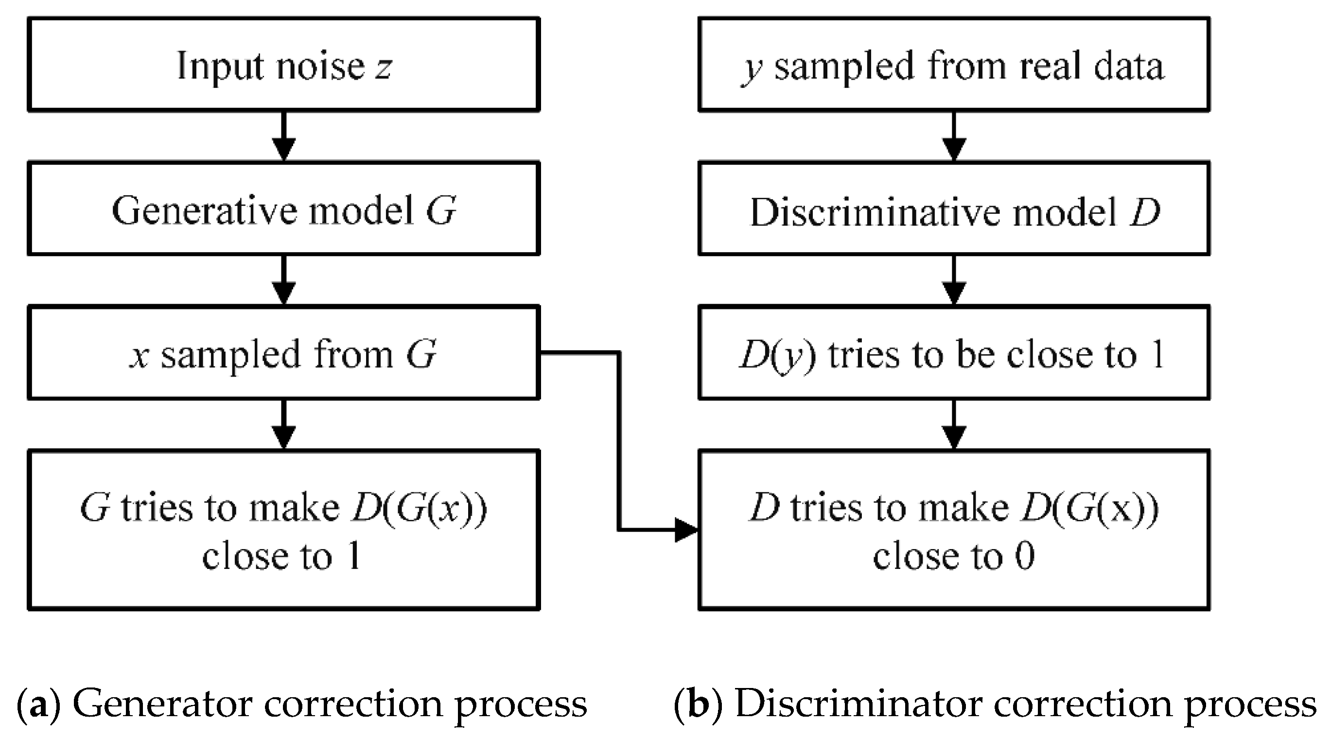
The GAN framework is a new deep framework for neural networks. It was proposed by Goodfellow et al. in 2014 and sparked a great proliferation of research in the field of deep learning. Because of the powerful image processing capabilities of GANs, they have a wide range of applications in the imaging processing field [20]. The basic GAN framework is shown in Figure 2.

As seen from this figure, a GAN offers improved efficiency by allowing two models to be trained at the same time: one is a generative model (G) used to capture the data distribution, and the other is a discriminative model (D) used to estimate samples. G and D learn in an adversarial manner. D models the real data, giving it the ability to identify the authenticity of such data. On the one hand, G generates various solutions in a certain space to train D’s discriminative ability. On the other hand, G attempts to find an optimal solution among these solutions that will be mistakenly identified by D as real data. Thus, a dynamic “game process” between G and D serves as the GAN optimization process. The equilibrium point in the game is the only solution. The corresponding model optimization function is shown in (8):

$$\begin{array}{c}\min \\ G\end{array}\begin{array}{c}\max \\ D\end{array}V\left(D,G\right)=E_{\chi ~P_g\left(x\right)} \lg D\left(x\right)+E_{\chi ~P_z\left(z\right)} \lg D\left(x\right)$$

(8)

Here, x is the real target image. z is the noise in the input to G. G(z) is the image generated by G. D(x) is the probability that D will judge that the real target image is x, and D(G(z)) is the probability that D will judge that G(z) is the real image x. To allow the generator to learn about the distribution P_g(x) from the data x, a prior variable P_z(z) of the input noise is defined.

2.3. Adaptive Model

Adaptive control is a subject involving the study of control problems for systems with uncertainties. An adaptive model can be regarded as a feedback control system that can intelligently adjust its own characteristics in response to environmental changes so that the system can work in an optimal state in accordance with certain set standards. Adaptive control is equivalent to conventional feedback control and optimal control in the sense that it is also a control method based on a mathematical model. The only difference is that adaptive control is based on less prior knowledge of the model and disturbances [23]. Therefore, it is necessary to continuously extract information about the model during the operation of the system so that the model can be gradually improved. Because research on adaptive control is highly similar to the principle of GANs, an adaptive model can be introduced into the GAN architecture.

Specifically, the network’s parameters can be continuously identified based on the input and output data of interest. When the network is in the initial iterative stage, the ability to extract image features is relatively lacking because the system has only just been put into operation. However, after a period of operation, as a result of real-time identification and control, the control system gradually adapts. The continuous improvement of the network’s parameters causes the control function synthesized based on this network to also continuously improve. In this sense, the control system possesses a certain adaptability. As the network’s generation and discrimination efforts continue to progress, through adaptive adjustment, the network will become more accurate and closer to the optimal solution, and finally, the network will have a powerful image segmentation functionality.

3. Image Segmentation Based on an AGAN

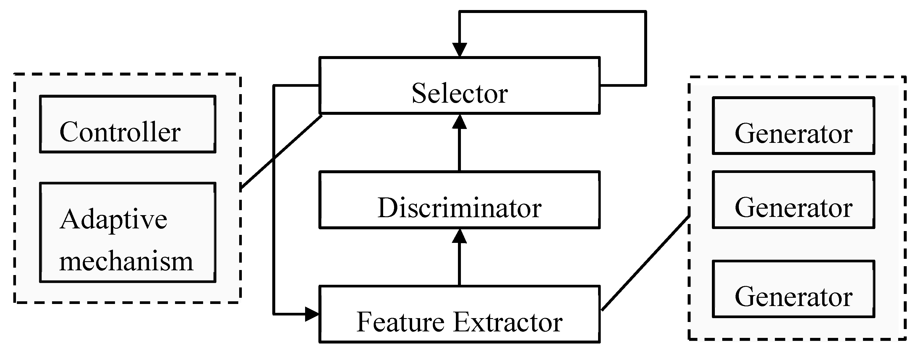
This section describes in detail the proposed image segmentation method based on an AGAN. First, the AGAN framework is introduced (Figure 3). Then, the specific implementation of each component, including the feature extractor, discriminator and selector, is introduced. Finally, the entire adaptive training and testing process of the algorithm is introduced.

3.1. Agan Framework

The AGAN framework is shown in Figure 3. An AGAN consists of three parts: a selector, a discriminator, and a feature extractor. The feature extractor contains multiple generators. The selector contains a controller and an adaptive mechanism. In this framework, the feature extractor extracts feature vectors of different dimensions. The extracted feature vectors are input into the corresponding discriminator to score the feature results. In this way, the feature extractor not only learns to extract dimensional characteristics through regular supervised training but also learns to extract features with better generalizability by deceiving the discriminator. To achieve more accurate feature descriptions and a faster iteration speed, the generators for different dimensions in the feature extractor are selectively promoted by the selector. The selector is used to adaptively coordinate the network. The selector is also used to adaptively select which dimensional features are considered.

The settings of the feature extractor and discriminator in this algorithm refer in part to the deployment of a GAN. The main purpose of the original GAN model is to fit the corresponding generator and discriminator functions to generate images. There is no restriction on the specific structures of the generator and discriminator. Due to the remarkable achievements of deep neural networks in image processing [26], the feature extractor and discriminator in this paper are both designed on the basis of neural network models. At the same time, to better retain the image details, the features extracted in two dimensions are also combined to make the segmentation more accurate after adaptive selection. A detailed introduction to the composition of and algorithm for each component in the framework is given in the following sections.

3.2. Feature Extractor

The feature extractor includes more than one feature generator. The purpose of the extractor is to extract deep image features at multiple levels to generate a new segmented image. To demonstrate the adaptive architecture proposed in this paper, the coordination of two networks is taken as an example. Therefore, it is assumed that the feature extractor contains two generators. The network structures of these two generators are the same, as shown in Figure 4.

In the encoder, first, the two generators each perform convolution operations on the input image with a 3 × 3 × 32 (filter size of 3 × 3, 32 filters, step size of 1) convolutional layer (Conv) and a 5 × 5 × 32 (filter size of 5 × 5, 32 filters, step size of 1) convolutional layer. Second, to avoid training failure caused by value shifts in the image distribution after convolution or during iteration, batch normalization operations (Batch) are performed in each convolutional layer after image convolution. Finally, the rectified linear unit (ReLU) activation function is used linearly to optimize the network performance. After the above three steps are repeated two or three times (as shown by the different numbers of different layers in Figure 4), a 2 × 2 × 2 (dimensions of 2 × 2, step size of 2) maximum pooling operation is performed. Because the sizes of the convolution kernels of the two generators are different, detailed information from the original image is extracted in multiple dimensions. Each time, the number of convolution kernels is doubled, and the size is reduced by half. After five encoding cycles, the extracted features enter the decoder.

In the decoder, a 2 × 2 upsampling operation is first performed. Then, the images obtained by copying and cropping before the maximum pooling layer and the image obtained by deconvolution in the corresponding layer are stitched together. Finally, the same convolution and batch normalization operations are performed in the corresponding layer. The above stitching, deconvolution, convolution, and batch normalization operations are repeated two or three times (as shown by the different numbers of different layers in Figure 4). Then, the results enter the next layer. Each time, the number of convolution kernels is reduced by half, and the size is doubled. After five decoding cycles, the decoded features enter the loss layer for the loss calculation. The loss guides changes to the parameters for the next iteration. The output of the penultimate layer is used as the input to the sigmoid layer. Then, the features are subjected to binary classification.

3.3. Discriminator

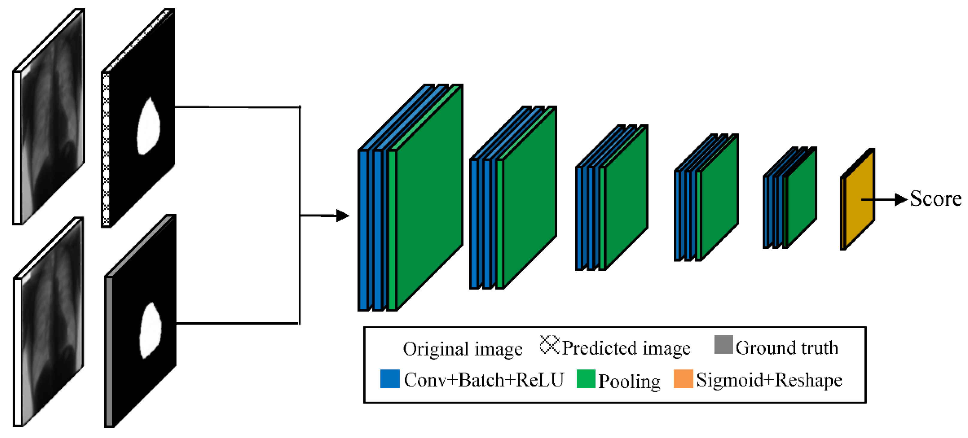
The discriminator in the network is used to identify whether a given segmentation result comes from the prediction of the model or is a real result. If the discriminator has a high level of discrimination but still cannot distinguish predicted results from real results, this indicates that the prediction model has a good expression or prediction ability. Since the feature extractor in the AGAN contains two generators, the discriminator here can also be used to evaluate the quality of these two generators. In the AGAN, the discriminator’s discrimination process for each generated result is the same as that of the discriminator in a GAN [27], and its structure is shown in Figure 5.

The left side of Figure 5 shows the two adversarial objects input into the discriminator, and the right side shows the structure of the adversarial network. The discriminator drives the adversarial learning process of the network based on two sets of input data. One set of data is the concatenation (Concat) of the original image and the gold standard segmentation, and the other set of data is the concatenation of the original image and the model-based segmentation result. The discriminator has a fully connected convolutional neural network structure, in which 3 × 3 × 32 (filter size of 3 × 3, 32 filters, step size of 1) filters are used to perform convolution operations to extract image features. As in the generators, the convolutional layers perform batch normalization operations after image convolution. The extracted features are optimized with the ReLU activation function (Conv + Batch + ReLU). The image features are downsampled with a pooling layer after two Conv + Batch + ReLU layers. At the same time, to reduce the loss of image information caused by the downsampling unit, the number of channels is doubled every time. The above operations are repeated five times. Finally, the results obtained after the above steps and reshaping are classified, and the results of the discriminator are output by the sigmoid function (Sigmoid + Reshape).

3.4. Selector

During the dynamic training process, the selector uses adaptive rules to select appropriate features and adjust the network training process and training parameters. The scores from the discriminator serve as the basis for the adaptive control rules. The structure of the selector is shown in Figure 6.

The adaptation process of the selector is accomplished through three loop paths. In the first loop, once the features have been extracted by the feature extractor, they are scored by the discriminator. The adaptive mechanism adjusts the controller to adjust the parameters of the feature extractor. In the second loop, during the training process, the parameters of the adaptive mechanism are adjusted in accordance with the data calculated by the feature extractor and the discriminator. In the third loop, the optimal features extracted by the feature extractor are selected. Through the adaptive mechanism, the features that can best describe the image are retained.

3.5. Training and Testing Process of the Agan

The principle of the entire AGAN framework is as follows: for a single network, if the score generated by the discriminator for a generator is low, this means that the output of this generator is far from the standard result and that the generator is still far from being underfitted. Then, the generator iterates for a certain number of steps before being scored by the discriminator again. For dual networks, the discriminator scores both networks. If one network has a high score, it is left unchanged for comparison, and the other network with a low score will then iteratively generate features to be scored and compared. Finally, combining the results for these two-dimensional features makes the network description more comprehensive. The algorithm process is as follows:

(1).

First, image features are extracted by the feature extractor.

(2).

Second, the features of different dimensions extracted by the two generators in the feature extractor are scored by the discriminator.

(3).

Finally, the selector adjusts the system through feedback and adaptive adjustment.

(4).

The above three steps are repeated until the network has a good representation ability; that is, the first loop of the adaptive adjustment process in the selector automatically terminates, and then the result of the calculation in the third loop is output.

During the testing process, the trained AGAN model is used to segment test images, and the third loop of the selector is used to determine the network output.

4. Experiments

In this section, the effectiveness of the proposed AGAN is verified through experiments. This section first introduces the JSRT (http://db.jsrt.or.jp/eng-01.php), the X-ray chest image database used in the experiments, and then specifies the experimental settings, including the indicators used to measure the quality of the segmentation results. The benchmark system used in the experiments, and the experiments conducted to compare the method proposed in this paper with other methods, are then introduced. The external tools used in this article are also described in the corresponding subsection. Finally, the experimental results are given in detail, including the specific network system performance and results analysis.

4.1. Image Database

Due to the low computational capacity of the computer used in this experiment (a 2.3 GHz Core i5 CPU with 8 GB of memory), the traditional JSRT database, which contains relatively few data, was chosen as the experimental object. The data in the JSRT were collected from 14 different medical institutions in the world, all confirmed by CT images and three radiologists. This database contains 247 manually labeled chest X-ray radiograph images. The image size is 2048 × 2048 pixels. As shown in Figure 4, each image is associated with a gold standard segmentation.

The 247 chest radiograph images were divided into a training group and a test group. For all algorithms, 50% of the images were used as the training sample, and the remaining 50% were used as the test sample. The experiments in this section were implemented based on the TensorFlow framework, and the image size was reduced to 128 × 128 pixels.

4.2. Evaluation Criteria

The segmentation accuracy of X-ray chest radiographs will affect the success of subsequent diagnosis and other image processing. Therefore, a variety of criteria were chosen to evaluate the performance of the algorithms.

The manual segmentation result was used as the gold standard for judging whether an algorithm classified the pixels correctly. Let TP denote the number of true positives, FN denotes the number of false negatives, FP denote the number of false positives, and TN denote the number of true negatives; then, the acc (accuracy), dice_coef (dice coefficient), sensitivity and specificity metrics can be calculated shown in (9)–(12), respectively.

$$\mathrm{acc}=\frac{TP}{TP+FP}$$

(9)

$$\mathrm{dice}\_\mathrm{coef}=\frac{2TP}{2TP+FP+FN}$$

(10)

$$\mathrm{sensitivity}=\frac{TP}{TP+FN}$$

(11)

$$\mathrm{specificity}=\frac{TN}{FP+TN}$$

(12)

4.3. Experimental Performance Comparison and Analysis

Specifically, the cardiac image segmentation results of the AGAN proposed in this paper were compared with the results of three commonly used image segmentation networks: SegNet [28], U-Net [18], and GAN [27]. Their segmentation results on the test set are shown in

Table 1. Comparisons of experimental data from different networks.

Network	Dice_Coeff	Acc	Sensitivity	Specificity
SegNet	92.41%	98.65%	88.86%	99.64%
U-Net	92.09%	98.59%	88.31%	99.64%
GAN	93.16%	98.75%	91.58%	99.48%
AGAN	94.06%	98.92%	92.25%	99.60%

. In the following, these results are analyzed from three perspectives.

The experimental result and the manually segmentation result dice similarity coefficient (dice_coeff) are the most important indicators to measure their similarity. The range of this value is 0 to 1. The best result is 1 and the worst result is 0. As can be seen from the results displayed in Table 1, the dice_coeff results of the AGAN are superior to those of the other three algorithms. The calculation method of acc in this case is to detect the proportion of the heart region in the segmented image as real heart region. This item can be used to check whether the image is over-segmented. It can be seen from the data in Table 1 that the extent of AGAN over-segmentation is not as significant as other methods. Specificity is the ratio of the cardiac correctly segmented area to all correctly segmented areas. Since the FN part is replaced by the smooth factor in the process of machine learning and testing, the result has a small deviation from the actual FN point. However, the smooth factor calculation rules adopted by each network are the same. The data in Table 1 show that the detection ability of the non-cardiac region is slightly weaker than the other three algorithms. More detailed comparisons and analyses are carried out from the following three aspects.

• Accuracy

Accuracy refers to the consistency between an algorithm’s segmentation results and the true segmentation results and is one of the most important indicators for evaluating segmentation algorithms. It can be seen from the experimental results that in terms of accuracy (acc), the network proposed in this paper outperforms the SegNet, U-net, and GAN models. Although the differences between them are not significant, the calculation formula for acc shows that there may be only a few false positive pixels for each of the various methods. In terms of dice_coeff, the result of 94.06% for the network proposed in this paper is 0.9% higher than that for the GAN model and 1.97% and 1.65% higher than those for the other two networks. Due to the small ratio of the area of the heart to the area of the entire X-ray chest radiograph for each segmented image, even a 0.9% improvement in dice_coeff is already significant. This can also be seen from Figure 7 and validates the previous assumption. The improvement in dice_coeff is mainly due to the increased sensitivity of segmentation. Since the algorithm proposed in this paper uses two dimensions to extract features, its sensitivity is more than 0.6% higher than that of the other algorithms. By contrast, there is not much difference in the specificity of the algorithms.

• Reliability

Reliability is considered to assess a segmentation method on the basis of statistical rules. It measures the impact of various changes on a segmentation method. To ensure the wide adaptability of an algorithm, reliability is an important evaluation measure. When the various neural networks above were trained on the same batch of images, their results show fluctuations because of different parameters. U-Net in particular, because it lacks a batch normalization layer, shows a large parameter dependence. Sometimes, because of improper initialization, some neurons of U-Net are unable to be activated during the training process, whereas other neurons are always activated, resulting in network training failure. In the case of nonadversarial training, the accuracy of the segmentation results fluctuates more than it does for other algorithms. In different training instances with the same parameters, the Dice coefficients on the training set and the test set fluctuated by approximately ±1.6%. SegNet is more stable than U-Net, and no training failure occurred for SegNet during the experiment. The results fluctuate by approximately ±1%. Because the GAN model and the AGAN model proposed in this paper are both based on the adversarial approach, these networks are relatively reliable. They showed fluctuations of less than ±1%. The four algorithms are compared below by visualizing the evaluation criteria of the network in the training process.

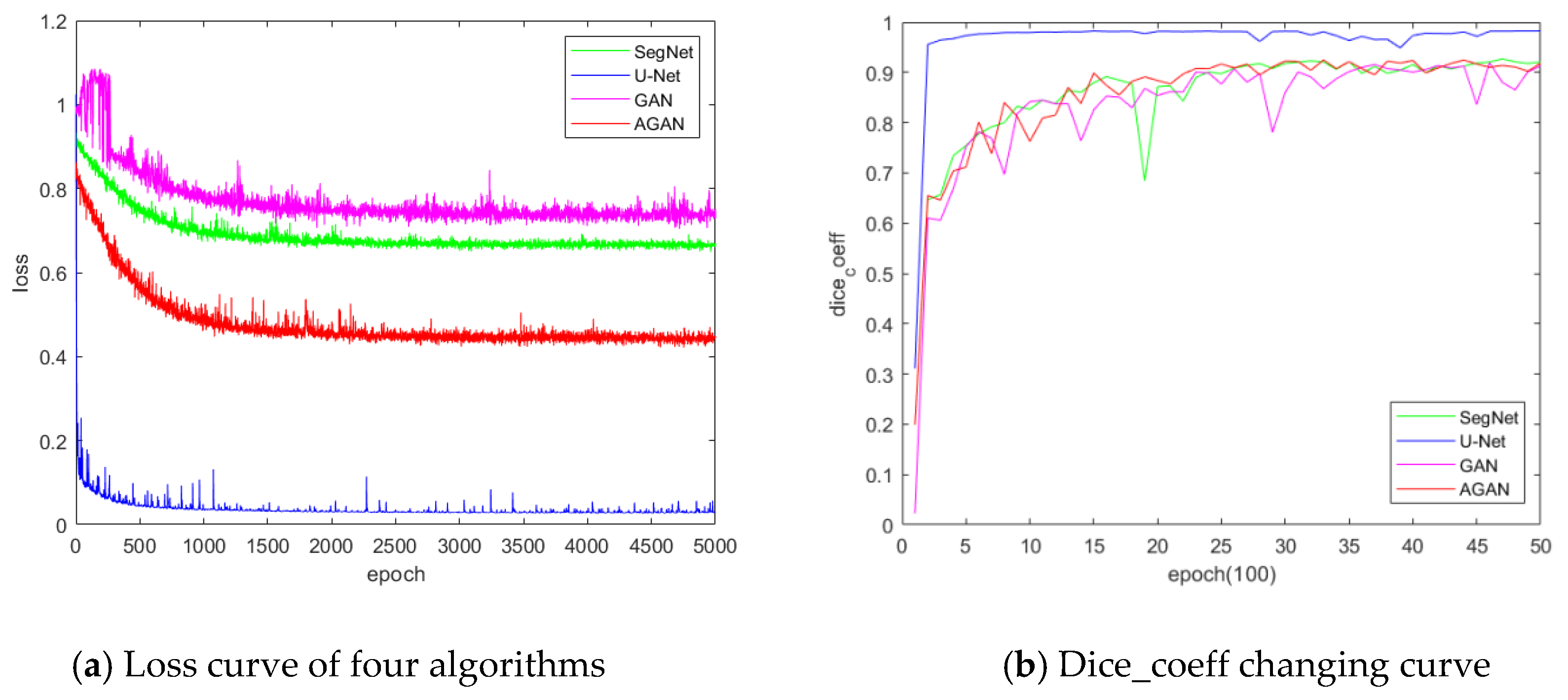
It can be seen from Figure 8 that both GAN and AGAN are based on adversarial networks, and the loss curves are relatively volatile, whereas loss curves of Segnet and U-net are more stable. The loss curve of AGAN drops faster than GAN, and tends to become stable earlier, and the performance in the later period is more stable. The speed of the dice_coeff is also improved faster than GAN. With reference to the results of the dice_coeff in the test set, there is no overfitting in the networks AGAN and GAN. This also confirms that algorithms based on GAN can avoid overfitting. It can also be found from the testing set results that U-net demonstrates a certain overfitting phenomenon.

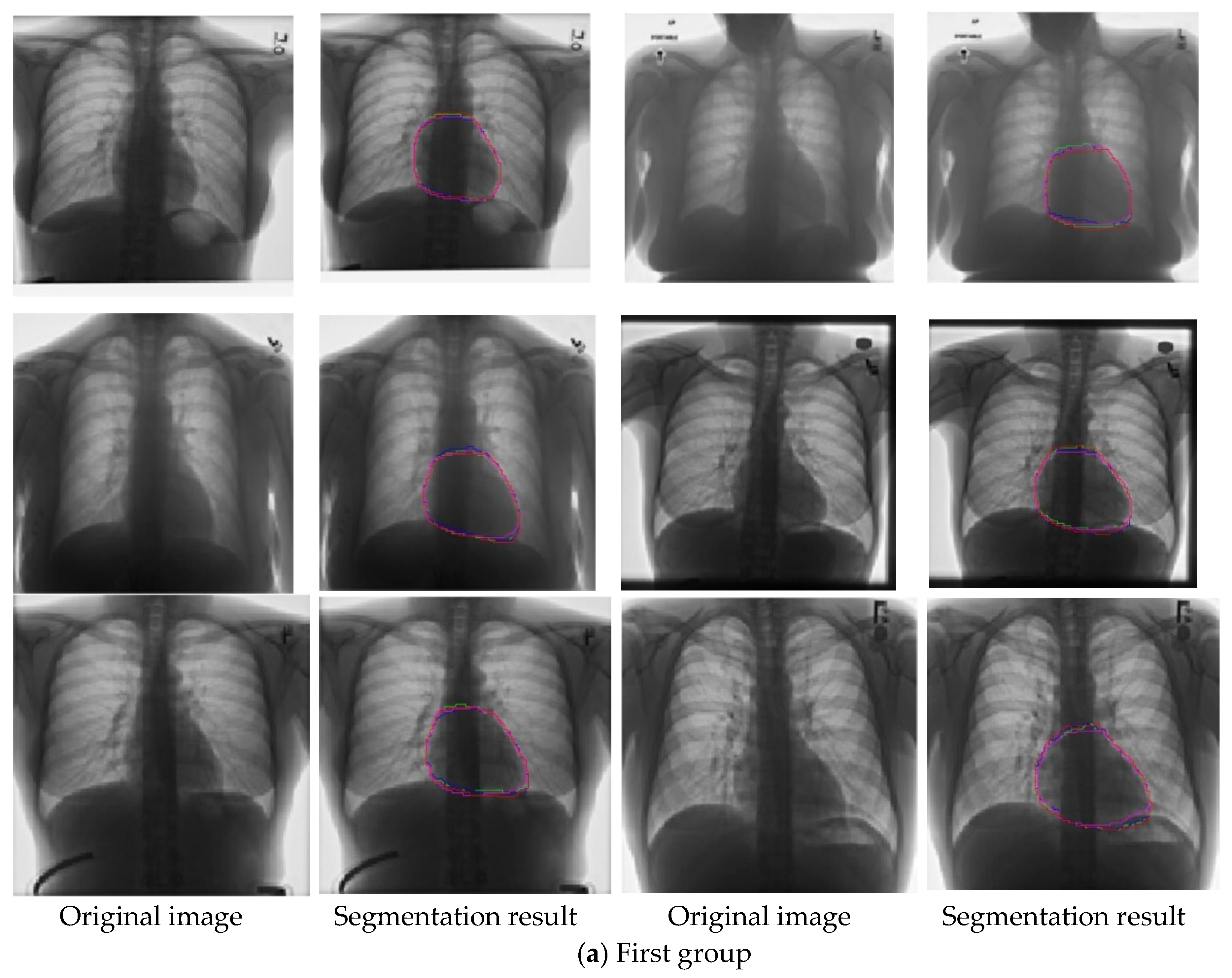
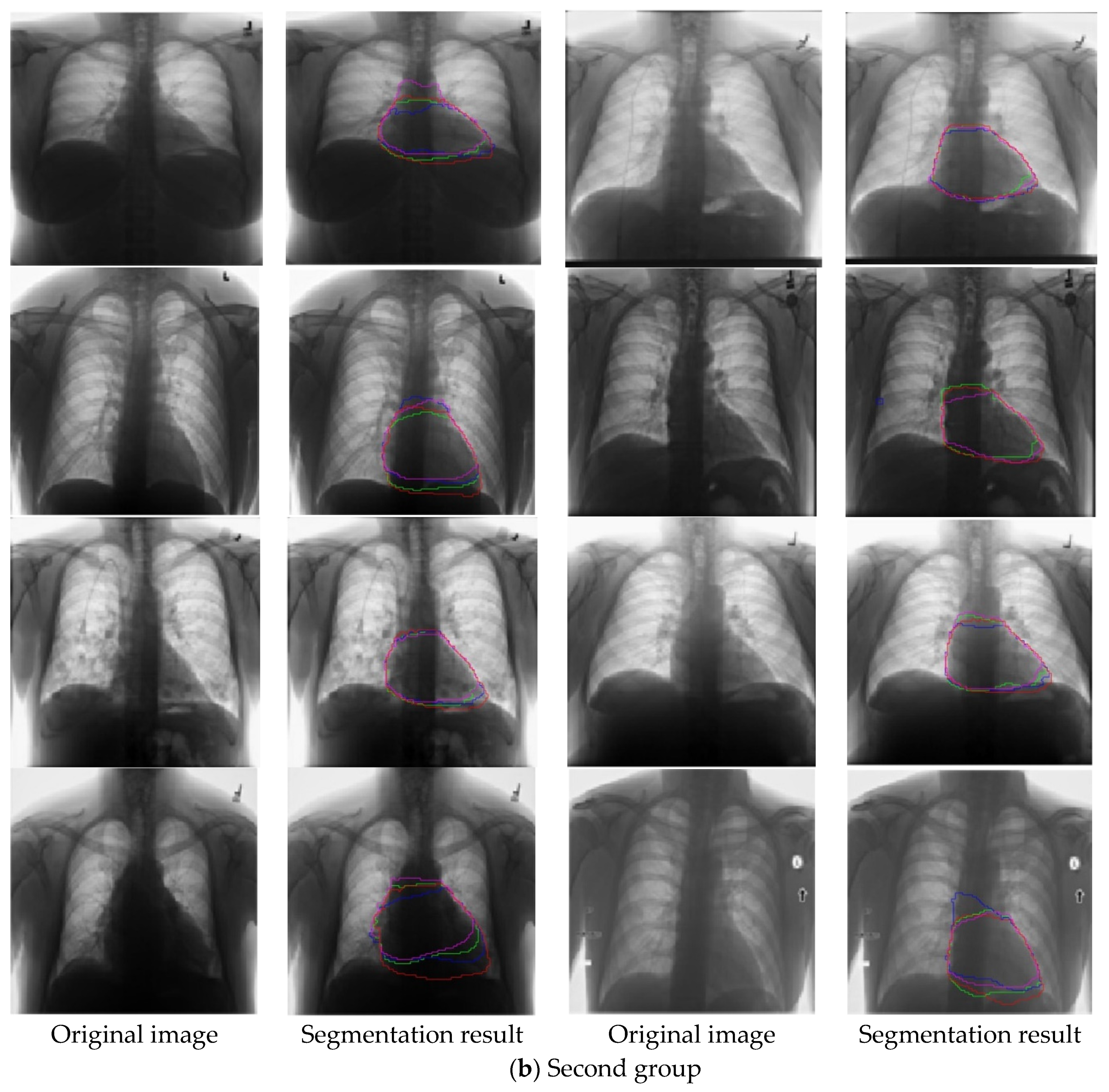
There are a total of 247 training and testing images in the JSRT database, which is a relatively small number, and which has only two groups of classifications. To illustrate the reliability of the network, the “chestX-ray8” (https://www.cc.nih.gov/drd/summers.html), the largest chest X-ray data set, was used as the experimental object. The database comprises 108,948 frontal view X-ray images of 32,717 unique patients. It includes images of atelelectasis, cardiomegaly, effusion, infiltration, mass, nodule, pneumonia and pneumathorax. We randomly selected 122 images from different disease categories and segmented them using different algorithms. Their results are shown in Figure 9.

Figure 9 contains three of the experimental results. In the figure, the red line outlines the segmented cardiac area with AGAN, the blue line outlines segmented cardiac area with segnet, the green line outlines the segmented cardiac area with unet, and the purple line outlines segmented cardiac area with GAN.

The database does not contain the results of manual segmentation as a reference. However, from the qualitative analysis of the experimental results, it can be concluded that AGAN is effective on X-ray images of non-JSRT data, and most of the results are also shown to be better than the other algorithms. In detail, the cardiac area in the first group of images is almost completely surrounded by the lungs and their edges are clear. All four algorithms have excellent segmentation results in this group of images. In the second group of images, the cardiac area is irregular in shape. In most cases, the AGAN segmentation result is slightly better than other methods. The conclusion is consistent with the experimental conclusion of the JSRT database. In the third group of images, it can be seen that while the segmentation results of the other networks are not desirable, the AGAN still performed well. This shows that the two generators can better extract features. Among the 122 pictures, four pictures failed to be segmented using AGAN, as shown in the last two figures in Figure 9. These graphs were also unsuccessfully segmented by using the other three methods. Therefore, the AGAN algorithm is reliable.

• Stability

Although the validation set was used to correct overfitting during the training of the above four networks, by comparing the results obtained on the test set and the training set, it can be initially determined that some networks still showed signs of overfitting. The scores (auc_pr + auc_roc) and other evaluation indexes for the four networks are shown in

Table 2. Comparisons of several performance indicators.

Evaluation Index	SegNet	U-Net	GAN	AGAN
STR	1.95	1.96	1.93	1.91
STE	1.93	1.91	1.90	1.91
BR	97.58%	97.65%	97.38%	98.37%
WR	69.18%	60.02%	70.18%	72.60%
N	3	4	4	1

STR = score on training set, STE = score on test set, BR = best result, WR= worst result, N = number of instances with a Dice coefficient of less than 0.8.

.

The best and worst results of the proposed AGAN on the test set are both better than those of the other three networks. The numbers of predictions with Dice coefficients below 80% are three, four, four, and one for the SegNet, U-Net, GAN, and AGAN models, respectively, which explains why cardiac segmentation with the AGAN is less likely to fail. It can also be seen that U-Net and SegNet achieved high scores on the training set but not on the test set. Even with a small amount of data, the difference is already significant. This is consistent with the fact that for these two networks, it cannot be determined during the training process when to stop training and whether there are overfitting problems. Because the GAN and AGAN architectures additionally include a discriminator, making the network more difficult to overfit due to the adversarial training process, their scores are not significantly different between the training set and the test set, and their generalization ability is good. The training curves of these two networks are shown in Figure 8. The AGAN reaches the equilibrium point earlier than the GAN does during training; moreover, the proposed network is more stable after reaching the equilibrium point, and it is not prone to overfitting.

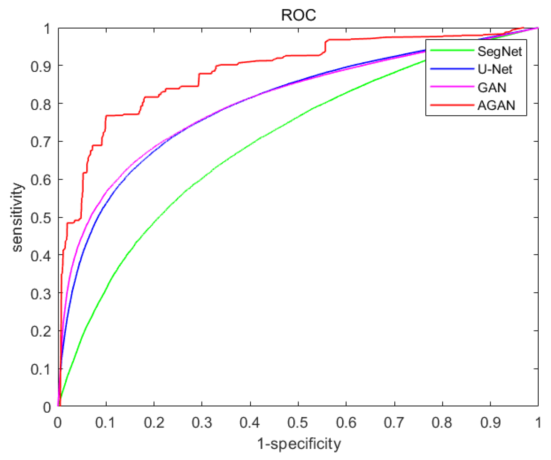
Finally, in order to illustrate the stability of the network, the ROC (Receiver Operating Characteristic) curves of the four networks are shown in Figure 10.

The horizontal axis in the ROC curve is 1-specificity (false positive rate), while the vertical axis is sensitivity (true positive rate). The calculation formula is shown in formulas (9) and (10). The FN is replaced by the smooth factor. If the smooth factor is small, the ROC curve is difficult to distinguish, so when drawing the ROC curve, the smooth factor takes a larger value. The ROC curves combine the true positive rate and the false positive rate graphically, which can accurately reflect the relationship amongst the various algorithms. The red curve in the figure does not intersect with other curves and is closest to the upper left corner. Therefore, the performance of AGAN is better than the other three networks. However, the ROC curves of the other networks are smoother. This is because AGAN has a selector to make a selection, so it cannot be smoothed on the excessive threshold.

5. Conclusions

This paper proposes an AGAN-based segmentation method for the task of X-ray chest image segmentation. The method combines the GAN framework with an adaptive learning algorithm. The whole framework includes three parts: a feature extractor, a discriminator and a selector. Taking a pair of GAN models as an example, the input image is segmented using an adaptive mechanism. First, a feature extractor based on two neural network models is used in the AGAN to generate feature vectors of specific dimensions from the input image. Second, a discriminator based on the same neural network structure is used to score the extracted dimensional features. Finally, an adaptive-control-based selector is implemented in the AGAN to dynamically adjust the training process and select optimal features. The discriminator is used to score the generator output and adaptively train the generators for different dimensions through an automatic adjustment algorithm so that the feature extractor will extract more representative feature vectors from the image input and achieve better generalizability. The experimental results obtained on a chest X-ray database show that the proposed AGAN is effective for X-ray chest radiograph segmentation and that its evaluation indexes are better than those of several other algorithms in general. The whole proposed system shows improved robustness and stability for image segmentation.

However, training the AGAN requires a large amount of calculation. In this study, only the coordination of two different-dimensional networks with a small amount of data was implemented. Our future work will first focus on larger data volumes and a wider range of applications. In addition, we will also improve the adaptive learning framework and algorithm, through measures such as introducing neural network layers that share parameters to enable the model to further learn to extract common features between different dimensions, in order to reduce the computational burden and achieve stable results with multiple coordinated networks.

References

1. Lesage, D.; Angelini, E.D.; Bloch, I.; Funka-Lea, G. A review of 3d vessel lumen segmentation techniques: Models, features and extraction schemes. Med. Image Anal. 2009, 13, 819–845. [Google Scholar] [CrossRef] [PubMed]
2. Yan, L.; Shuang, Q.T.; Bin, C.Z. An Automated Calculation of Cardiothoracic Ratio on Chest Radiography. Chin. J. Biomed. Eng. 2009, 28, 149–152. [Google Scholar]
3. Toth, D.; Panayiotou, M.; Brost, A.; Behar, J.M.; Rinaldi, C.A.; Rhode, K.S.; Mountney, P. 3D/2D Registration with Superabundant Vessel Reconstruction for Cardiac Resynchronization Therapy. Med. Image Anal. 2017, 42, 160. [Google Scholar] [CrossRef] [PubMed] [Green Version]
4. Hatt, C.R.; Speidel, M.A.; Raval, A.N. Real-Time Pose Estimation of Devices from X-ray Images: Application to X-ray/Echo Registration for Cardiac Interventions. Med Image Anal. 2016, 34, 101–108. [Google Scholar] [CrossRef] [PubMed] [Green Version]
5. Yan, P.; Zhang, W.; Turkbey, B.; Choyke, P.L.; Li, X. Global structure constrained local shape prior estimation for medical image segmentation. Comput. Vis. Image Underst. 2013, 117, 1017–1026. [Google Scholar] [CrossRef]
6. Yu, H.; He, F.; Pan, Y. A novel segmentation model for medical images with intensity inhomogeneity based on adaptive perturbation. Multimed. Tools Appl. 2019, 78, 11779–11798. [Google Scholar] [CrossRef]
7. Iakovidis, D.K. Versatile approximation of the lung field boundaries in chest radiographs in the presence of bacterial pulmonary infections. In Proceedings of the IEEE International Conference on Bioinformatics & Bioengineering IEEE 2008, Athens, Greece, 8–10 October 2008. [Google Scholar]
8. Umehara, K.; Ota, J.; Ishimaru, N.; Ohno, S.; Okamoto, K.; Suzuki, T.; Shirai, N.; Ishida, T. Super-resolution convolutional neural network for the improvement of the image quality of magnified images in chest radiographs. In Proceedings of the Conference on Medical Imaging—Image Processing, Orlando, FL, USA, 12–14 February 2017. [Google Scholar]
9. Becker, H.C.; Nettleton, W.J.; Meyers, P.H.; Sweeney, J.W.; Nice, C.M. Digital Computer Determination of a Medical Diagnostic Index Directly from Chest X-Ray Images. IEEE Trans. Biomed. Eng. 1964, BME-11, 67–72. [Google Scholar] [CrossRef]
10. Hall, D.L.; Lodwick, G.S.; Kruger, R.; Dwyer, S.J. Computer diagnosis of heart disease. Radiol. Clin. N. Am. 1972, 9, 533–541. [Google Scholar]
11. Nakamori, N.; Doi, K.; Sabeti, V.; MacMahon, H. Image feature analysis and computer-aided diagnosis in digital radiography: Automated analysis of sizes of heart and lung in chest images. Med. Phys. 1990, 17, 342. [Google Scholar] [CrossRef]
12. Viergever, M.A.; Romeny, B.H.; van Goudoever, J.B. Computer-aided diagnosis in chest radiography: A survey. IEEE Trans. Med. Imaging 2001, 20, 228–241. [Google Scholar]
13. James, S.D.; Nicholas, A. Medical image analysis: Progress over two decades and the challenges ahead. IEEE Trans. Pattern Anal. Mach. Intell. 2000, 22, 85–106. [Google Scholar]
14. Kass, M.; Witkin, A.; Terzopoulos, D. Snakes: Active Contour Models. Int. J. Comput. Vis. 1988, 1, 321–331. [Google Scholar] [CrossRef]
15. Behiels, G.; Vandermeulen, D.; Maes, F.; Suetens, P.; Dewaele, P. Active Shape Model-Based Segmentation of Digital X-ray Images. Lect. Notes Comput. Sci. 1999, 1679, 128–137. [Google Scholar]
16. Cootes, F.T.; Edwards, G.J.; Taylor, C.J. Active appearance models. IEEE Trans. Pattern Anal. Mach. Intell. 2001, 23, 681–685. [Google Scholar] [CrossRef] [Green Version]
17. Van Ginneken, B.; Frangi, A.F.; Staal, J.J.; ter Haar Romeny, B.M.; Viergever, M.A. Active shape model segmentation with optimal features. IEEE Trans. Med. Imaging 2002, 21, 924–933. [Google Scholar] [CrossRef] [PubMed]
18. Alex, K.; Sutskever, I.; Hinton, G.E. ImageNet Classification with Deep Convolutional Neural Networks. Commun. ACM 2017, 60, 84–90. Available online: http://www.cs.toronto.edu/~hinton/absps/imagenet.pdf (accessed on 22 June 2020).
19. Olaf, R.; Fischer, P.; Brox, T. U-Net: Convolutional Networks for Biomedical Image Segmentation. In Proceedings of the 18th International Conference on Medical Image Computing and Computer-Assisted Intervention (MICCAI), Munich, Germany, 5–9 October 2015; pp. 234–241. [Google Scholar]
20. Goodfellow, I.; Pouget-Abadie, J.; Mirza, M.; Xu, B.; Warde-Farley, D.; Ozair, S.; Courville, A.; Bengio, Y. Generative adversarial nets. In Proceedings of the 2014 Conference on Advances in Neural Information Processing Systems 27; Curran Associates, Inc.: Montreal, QC, Canada, 2014; pp. 2672–2680. [Google Scholar]
21. Dan, P.; Longfei, J.; An, Z.; Xiaowei, S. Applications of Generative Adversarial Networks in medical image processing. J. Biomed. Eng. 2018, 6, 970–976. [Google Scholar]
22. Chen, C.; Dou, Q.; Chen, H.; Heng, P.A. Semantic-Aware Generative Adversarial Nets for Unsupervised Domain Adaptation in Chest X-Ray Segmentation. In Machine Learning in Medical Imaging Workshop with MICCAI 2018; Springer: Cham, Switzerland, 2018. [Google Scholar]
23. Li, X.; Wang, W.; Sun, W. Multi-model Adaptive Control. Control. Decis. 2000, 15, 390–394. [Google Scholar]
24. Lv, Y.; Na, J.; Yang, Q.; Wu, X.; Guo, Y. Online adaptive optimal control for continuous-time nonlinear systems with completely unknown dynamics. Int. J. Control. 2016, 89, 99–112. [Google Scholar] [CrossRef] [Green Version]
25. Affonso, C.; Rossi, A.L.D.; Vieira, F.H.A.; de Leon Ferreira de Carvalhob, A.C.P. Deep learning for biological image classification. Expert Syst. Appl. 2017, 85, 114–122. [Google Scholar] [CrossRef]
26. Ma, Z.; Wu, X.; Wang, X.; Song, Q.; Yin, Y.; Cao, K.; Wang, Y.; Zhou, J. An iterative multi-path fully convolutional neural network for automatic cardiac segmentation in cine MR images. Med. Phys. 2019, 46, 12. [Google Scholar] [CrossRef] [PubMed]
27. Guo, Z.; Li, X.; Huang, H.; Guo, N.; Li, Q. Deep Learning-based Image Segmentation on Multi-modal Medical Imaging. IEEE Trans. Radiat. Plasma Med. Sci. 2019, 3, 162–169. [Google Scholar] [CrossRef]
28. Xia, K.; Yin, H.; Qian, P.; Jiang, Y.; Wang, S. Liver Semantic Segmentation Algorithm Based on Improved Deep Adversarial Networks in combination of Weighted Loss Function on Abdominal CT Images. IEEE Access 2019, 7, 96349–96358. [Google Scholar] [CrossRef]
Figure 1. The structure of a convolutional neural network.
Applsci 10 05032 g001
Figure 2. Generative adversarial network (GAN) framework.
Applsci 10 05032 g002
Figure 3. Adaptive generative adversarial network (AGAN) framework.
Applsci 10 05032 g003
Figure 4. The network structure of the generators.
Applsci 10 05032 g004
Figure 5. The network structure of the discriminator.
Applsci 10 05032 g005
Figure 6. The structure of the selector.
Applsci 10 05032 g006
Figure 7. Comparison of three groups of AGAN segmentation results with the results of other methods.
Applsci 10 05032 g007aApplsci 10 05032 g007b
Figure 8. The performance comparison of the four networks during the training process.
Applsci 10 05032 g008
Figure 9. Comparison of three groups of AGAN segmentation results with the results of other methods.
Applsci 10 05032 g009aApplsci 10 05032 g009bApplsci 10 05032 g009c
Figure 10. ROC curve of four algorithms.
Applsci 10 05032 g010