Abstract
Bi-layered metallic bending tubes are widely used in extreme environments. The spring-back prediction theory for precise forming of such tube configuration is lacking. The layered coupling causes complex section internal force and new boundary conditions. This work proposed a theoretical prediction model of bimetallic tubes’ spring-back under computer numerically controlled (CNC) bending. This model calculated the spring-back angle by importing two new parameters—the composite elastic modulus (Ec) and the composite strain neutral layer (Dε). To investigate Dε, the neutral layer shifting extraction method was proposed to get the shifting value from finite element simulations. Simulations and full-scale bending experiments were carried out to verify the reliability of this prediction model. The theoretical results are closer to the experimental results than the finite element (FE) results and the theoretical results neglecting neutral layer shifting. The change of spring-back angle with the interlaminar friction coefficient was investigated. The results indicated that the normal mechanical bonding bimetallic tube with an interlaminar friction coefficient below 0.3 can reduce spring-back.
1. Introduction
Bi-layered metallic tubes and their elbow components play an important role in changing the flow direction and improving the flexibility of wiring in pipeline systems [1,2,3]. As related industries are developing and transforming, many new demands such as corrosion protection, wear resistance, impact resistance, thermal insulation, electric insulation, low cost, lightweight, etc. have appeared. Compared with single-metallic tubes, bimetallic tubes can meet the new requirements better and have gradually been applied for engineering [4,5,6,7]. By making full use of the optimum of different materials, bimetallic tubes can reduce the use of precious metals, lighten the weight of pipes, and reduce production and transportation costs. Therefore, bimetallic tubes are in wide use in the automobile, ship, aerospace, petrochemical, nuclear power, and military industries [8,9,10,11].
The elbow components are formed by cold processing of straight metallic tube blanks. The bending forming quality is directly related to the assembly accuracy, operation safety, and flow stability. Usually, three indexes are used to reflect the forming quality—wall thickness thinning [12,13,14], wrinkling [15,16,17,18], and spring-back. At present, studies of bimetallic tube bending forming almost focus on analysis of wall thickness variation and wrinkling caused by complex bulking instability under the interaction of two or more layers. Guo et al. [19] proposed a model about the wall thickness distribution of Cu-Al bi-layered tube. Their research indicated that the wall thickness distribution of bimetallic tube tended to be more uniform than single-layered tube. Wang and Li [20] analyzed the inner wall thickness variation of double-layered tube in hydrobending. It was found that the maximum thickness reduction occurred at a nearby point rather than the center point of the outer arc because the point with the biggest axial stress moved toward the tube ends. Apart from the common defects such as cracking caused by wall thickness changes and wrinkling due to instability, bimetallic tubes have hidden defects compared with single-layered metallic tubes. This means that the inner layer may separate from the outer layer or collapse while the bimetallic tube looks normal on the outside. Gavriilidis et al. [21] studied the buckling of offshore steel-lined pipes numerically subjected to monotonic bending. The main conclusion was that low or moderate internal pressure can improve the bending performance such as ovalization, detachment of the thin-walled inner pipe from the outer pipe, and liner buckling of lined pipes. Teng et al. [22] analyzed the wrinkling behaviors of carbon steel/Al-alloy bi-layered tubes with different thickness ratios and internal pressures under hydro bending. The bifurcation instability of inner tube and the limit load instability of outer tube were also noticed. It followed that internal pressure can delay the separation and wrinkling of bimetallic tube’s inner layer efficiently.
The spring-back behaviors of bimetallic elbow components after computer numerically controlled (CNC) bending is an important aspect of the forming defects prevention. So far, scholars have carried out a lot of mature theoretical models and reliable experimental results about tubes’ spring-back behaviors. Zhan et al. [23] established an analytic elastic-plastic tube bending spring-back model based on static equilibrium condition considering the variations of some parameter in the bending process. Zhang et al. [24] proposed a semi-analytical method for the spring-back prediction of thick-walled 3D tubes. The discretization and approximation were implemented on the tube axis to derive the deformation parameters and the relationship between parameters in bending process and those after spring-back was defined. Wu et al. [25] investigated the spring-back of spatial tubes under different loading modes and hardening materials. The conclusion was that the spring-back increased with the increasing of loading index , so evaluating reasonably can improve the precision of prediction. In order to avoid the excessive error caused by the assumptions in the theoretical analysis and reduce the difficulty of solving analytical models, many researchers use the numerical simulation method to obtain the engineering solution of the rebound problem. Li et al. [26] investigated the geometry-dependent spring-back behaviors of thin-walled tube upon cold bending. They aimed at two geometry parameters—tube diameter and wall thickness . Song et al. [27] predicted spring-back by combining explicit and implicit schema. They carried out the influence of numerical parameters such as element type, number of elements through thickness, and damping factor on prediction accuracy and simulation efficiency. Dan and Zhang [28] established a simulation model to define the relationships between process parameters and spring-back angle. Controlling functions for plastic elongation and spring-back angle are also given. The existing research objects about the rebound of multi-layer composite components are strip, plate, and heterogeneous bellows. Shayan et al. [29] studied the effects of sheet thickness and position on spring-back of a stainless-steel clad aluminum sheet’s V-bending though the nonlinear FEM. Their research addressed three material models—isotropic, cyclic, and Johnson–Cook hardening. Liu and Xue [30] derived a simplified analytical model to calculate the bending moments of sandwich sheets, and the model was applied to predict the spring-back after bending. The spring-back angle is mainly determined by the skin sheet’s mechanical properties. Liu et al. [31] conducted a comparative study on the profile shape spring-back of bi-layered nonhomogeneous bellows. Their results included the degree of U-shape deformation and the spring-back tendency with the variation of some parameters like layer number, material properties, etc. As for bimetallic tubes, because of the complex section characteristics, new boundary conditions are added to their spring-back on the base of geometrical and material nonlinearity. It is harder to solve the rebound problem. The spring-back theory, prediction model, and compensation method of bi-layered metallic tube are all lacking.
The resolution of tube bending spring-back needs to transfer external forces into internal stress. The neutral layers are the geometrical zero points of stress and strain, the researches of whose positions make sense in the bending problems. Under pure bending, the transient stress and strain neutral layers all move toward bending center as the bending curvature increases. The transient stress of the neutral layer’s shifting amount is greater than transient strain of the neutral layer if the elastic deformation can be neglected, which was mentioned by E [32]. To reduce the calculative difficulties and obtain the stress–strain relationship easily, it is generally assumed that the neutral layers coincide with the center layer of the tube blank. However, due to the high complexity caused by the coupling deformation of the two layers, the neutral layer invariance assumption may lead to more obvious errors in bimetallic tube bending spring-back. In this paper, it was proved that the strain neural layers of outer layer and inner layer are almost coincident in the effective bending range. The neural layer shifting can be expressed by a composite strain neutral layer (). A novel neutral layer shifting extraction (NLSE) method was firstly proposed to ascertain the position of . Via the NLSE method applied to simulation results as well as regression analysis, the function of about the parameters such as bending radius, bending angle, tube size, etc. was derived. In addition, a composite elastic modulus (Ec) was proposed to describe the spring-back behaviors of bimetallics. The theoretical spring-back prediction model of bimetallic bending tubes was established considering the neutral layer shifting, which can be used to calculate the spring-back angle of bi-layered tubes in CNC bending process. The experimental bimetallic bending tubes formed by King-Mazon PB50CNC tube bender verified the prediction results’ accuracy.
2. Theoretical Model of the Bimetallic Tube Bending Spring-Back
2.1. Principle of the Bimetallic Tube Spring-Back
The stress–strain relationship in the process of tube bending can be described simply as a power hardening model. Assuming that unloading is a completely elastic deformation process, the elastic-plastic deformation of tube bending is shown in Figure 1. Point M is the dividing point between elastic deformation and plastic deformation in the loading process. Point N is the machining maximum stress point. The load gradually increases from point O to point N to meet the requirements of bending processing. Unloading from point N to point P. The position of point P indicates that there are residual stress and residual strain in the component.
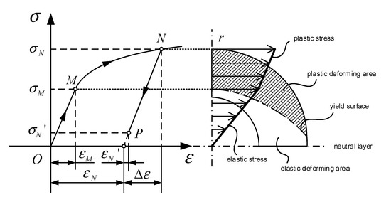
Figure 1.
Bending loading (unloading) process and deformation area of cross section.
Considering the fiber layer with radial distance y from the stress neutral layer at point N shown in Figure 2. The micro internal force in each layer of the circular section forms a group of spatial parallel force systems. Since the bending moment on the tube is zero after unloading, the stress change during unloading satisfies the following relationship:
where MO denotes bending moment on the tube when loaded to the maximum stress.

Figure 2.
Differential of circular section and spring-back diagram of bending tube.
Ignoring the residual stress and the delayed rebound after instantaneous rebound, the unloading process line can approximately extend to the point where the stress is zero along the straight line NP. Assuming that the stress neutral layer and the strain neutral layer at point N coincide, the variation of strain corresponding to the variation stress above is
where D denotes curvature radius of the stress neutral layer at point N, denotes curvature radius of the central axis of the tube before spring-back, and denotes curvature radius of strain neutral layer after spring-back.
In the analysis of the unloading process above, the relationship between and . can also be calculated through the material model and yield strength theory during tube loading. Further, can be solved.
According to the volume incompressible condition, the unloading spring-back angle is
Compared with the integrated tube fittings, the bimetallic tube is composed of two layers of materials, each layer of which has its own elastic modulus. When the elastic modulus of the two layers is not equal, the spring-back behavior cannot perform following their own elastic modulus due to the mutual restraint between two layers. Since the effective bending requirement of the bimetallic tube is that the two layers do not separate in the whole forming process, the composite tube’s spring-back behaviors can be regarded as the integral tube’s elastic deformation following a certain composite elastic modulus Ec.
Consider a double-layer tube with elastic tension or compression deformation under axial force F. Figure 3 illustrates the situation. The strain on each part of the tube is equal, which is expressed by . According to the fact that the axial forces on any circular section are equal, Formulas (5) and (6) can be obtained, and Formula (7) for calculating the composite elastic modulus of the double-layer tube can be derived.
where and σ2 represent the stress in the outer layer and the inner layer, and represent circular section’s area of the outer layer and the inner layer, E1 and represent the elastic modulus of the outer material and the inner material, and represent wall thickness of the outer layer and the inner layer, and denotes the radius of the outermost layer.
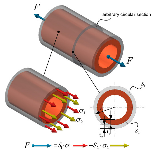
Figure 3.
Bi-layered straight tube under axial elastic tension or compression.
2.2. Uploading Moment of the Bimetallic Tube
The stress–strain relationship of the two layers of metal materials can be described by the following power hardening model because of its practicality and accuracy. Different parameters of the inner layer and outer layer are distinguished by subscripts. The symbol with subscript 1 indicates the parameters of the outer layer while subscript 2 indicates inner correspondingly.
where denotes strength coefficient, nj denotes hardening index, and denotes yield strength.
The tangential stress along the bending path is the main factor effecting the plastic tension and compression deformation and the tangential strain is the main characterization of elastic recovery. To simplify the analytical process, the non-uniform deformation in bending has been ignored. It is also assumed that the tangential stress–strain relationship along the bending path is consistent under tension and compression, which conforms to the power hardening material model. Considering a certain state with a fixed bending radius and angle, the stress distribution on the circular section approximately exhibits lamellar layers parallel to the stress neutral layer. The stress value gradually increases from the neutral layer along the radial direction of the circular section. So, it can be assumed that only elastic deformation occurs in the volume layer near the neutral layer. As the section radius increases, plastic deformation happens to occur in the volume layer far from the neutral layer. For multi-layer composite bending tubes, each layer of material on the circular section conforms to this feature. According to this, the circular section deformation area of the bimetallic tube in plane CNC bending can be divided into elastic deformation region and plastic deformation region, as shown in Figure 4.
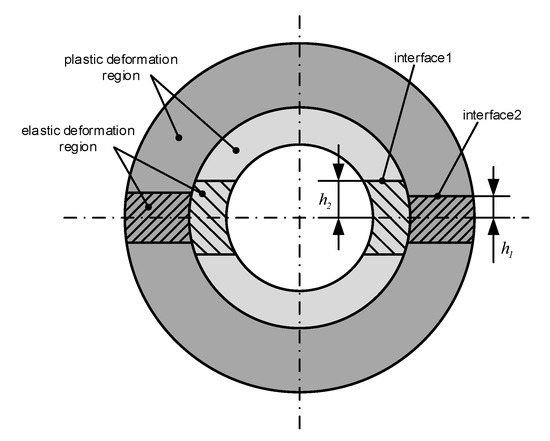
Figure 4.
Section deformation area of the bimetallic bending tube.
There are interfaces between the elastic deformation region and the plastic deformation region of each layer. The position of the interfaces is determined by the yield strength of materials respectively and symmetry about the neutral layer. To simplify the calculation, the wall thinning and the flattening phenomena have been neglected. The stress neutral layer and the geometry intermediate are regarded as coincident when deriving the uploading moment. By setting the distance between interfaces and the strain neutral layer as , the position of interfaces can be expressed as follows:
and denote the moments of the elastic deformation region and the plastic deformation region. By the integration of the differential layer with z distance from the strain neutral layer, the banding moment under a certain state is
2.3. NLSE Method
There are two special curved surface layers, namely stress neutral layer and strain neutral layer, existing in the bending tubes. The positions of these two layers are shifting instantaneously as the bending parameters changing. The instantaneous strain neutral layer is a fiber layer whose arc length is equal to the original length of tube blank and tangential strain is zero. Similarly, the instantaneous stress neutral layer refers to the fiber layer with zero tangential tensile and compressive stress. The former has geometric significance and the later has physical significance. In the bending process, both neutral layers move toward the bending center, and their movement is not synchronous.
The effective requirement of the bending process for the mechanical combined bimetallic tube is that the inner and outer layers will not separate during the loading and rebound process. The contact surface is always close without gaps. On the circular section, due to the different material properties of the two layers, the stress distribution in each layer exhibits discontinuities at the contact between layers as shown in Figure 5a. According to the requirements of effective bending, the strain property of the bi-layered tube is consistent with that of a single-layered tube. The section strain will increase continuously with the increase of section radius. As shown in Figure 5b, the strain is continuous and the transition at the interface between two layers is smooth. It is evident that the zero-point layer of equivalent strain is close to the inner side of bending, which proves the accuracy of the above analysis.
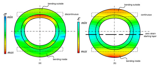
Figure 5.
Von Mises stress (a) and strain (b) of the bimetallic bending tube section.
According to the continuity of the section strain, there must be a composite neutral layer strain of in the bending process of the composite tube whose strain is zero. In order to locate the strain start, a meaningful strain component distributing regularly along the section radius direction should be focused. Because the tube can deform freely only on the tangential direction without restricting by bending dies, the tangential strain has important value of reference. There is a geometric relationship that the tangential strain increases linearly along the section radius to the inside and outside sides of the bending. Assuming the bimetallic tube is on the plane stress state, the first principal strain is equivalent to tangential strain. The tangential strain on the bending section is illustrated in Figure 6. It is obvious that the neutral layer of strain has shifted to the bending center.
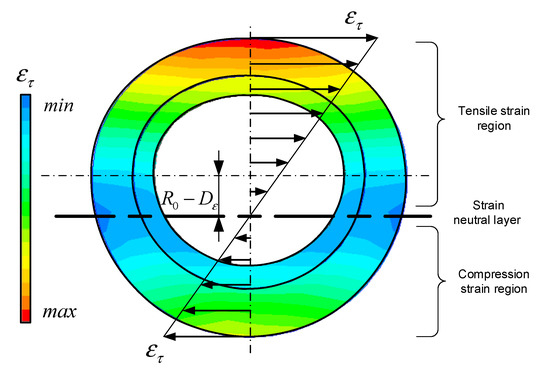
Figure 6.
Tangential strain of the bimetallic bending tube section.
In engineering practice, the neutral layer lacks effective and direct representation on the circular section of the elbow. Accordingly, it is difficult to obtain the specific position of the neutral layer through physical experiments. Therefore, the method of extracting the neutral layer from the FE simulation results based on the ANSYS Workbench platform is considered. Through the post-processing of simulation results provided by the platform, the specific position of the composite strain neutral layer can be obtained. Take the lines parallel to the central axis of the bending tube at the outermost and innermost walls, respectively, and set them as and . Due to the numerical nature of FE, and consist of uniform discrete points respectively. Points on have one-to-one correspondence with points on . The simulation results to be extracted are listed in Table 1.

Table 1.
Directly extracted simulation results.
It is assumed that the XY plane is the bending plane. The outline of the bimetallic tube can be drawn according to the point coordinates on and . Setting the tangential strain as the value of Z axis coordinate of each point of and . The strain value in the tensile area is positive and the strain value in the compression area is negative. The space curve f1 and indicating the tangential strain on the outermost and innermost walls can be drawn.
Because the tangential strain on the cross profile of the bending section distributes linearly along the radial direction, selecting some points on bending section and connecting a point on and the corresponding point on , the neutral layer locates at the intersection of the line and XY plane. denotes the distance between Pk and the bending center . This parameter is used to express the location of the strain neutral layer on this section.
In the bending section, m+1 pairs of points are taken to calculate the neutral layer positions, and the mean value is taken as the total strain neutral layer position. As follows, the curvature radius and shifting value of the strain neutral layer in the bending section can be expressed by and Sε. Figure 7 is the process diagram.
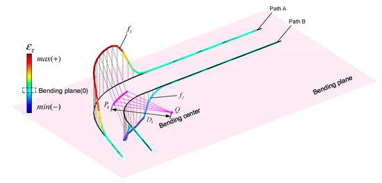
Figure 7.
Process diagram of neutral layer shifting extraction (NLSE).
3. Regression Analysis of Neutral Layer Shifting
3.1. Experimental Design
The composite strain neutral layer shifting of the bimetallic tube is influenced by many factors such as materials, the composite mode, processing parameters, bending conditions, the tube’s geometric parameters, interlaminar coupling effect under bending, and many other aspects. To simplify the analysis and the shifting model, it is assumed that the implications of materials and processes can be ignored. Several factors, which can comprehensively summarize the bending conditions, geometric parameters, and interlaminar coupling effect, are selected for experiments.
Considering the correlation between those single parameters such as bending die radius, outer diameter and total thickness, several kinds of ratios are set as experimental factors. There are six factors including bending angle, outer diameter, relative bending radius (the ratio of bending die radius to outer diameter), diameter-thickness ratio (the ratio of outer diameter to total thickness), layered thickness ratio (the ratio of outer thickness to inner thickness), and interlaminar friction coefficient. The bending angle and relative bending radius denote bending conditions. The outer diameter, the diameter-thickness ratio, and the layered thickness ratio denote the tube size—that is, the geometric parameters of the tube. The interlayer friction coefficient denotes the coupling effect of the double-layered materials in the bending. The commonly used combination of metal materials, i.e., outer 202 stainless steel and inner Q235 carbon steel, is selected for coreless bending simulation experiments. The factors and levels are shown in Table 2.
Table 2.
Experimental design factors and levels.
The orthogonal experimental design is an effective method to study the multi factor-level sample data. It can reflect the experimental data in a certain range uniformly and roundly. Due to the nonexistence of a typical orthogonal table containing the above factors and levels, SPSS statistic software is taken to generate the experimental schemes. The 49 groups of orthogonal experimental schemes with all factors and different levels are listed. Simulation is carried out according to each group of experimental conditions. The strain neutral layer shifting Sε is extracted from the simulation results by using the NLES method referred to in Section 2.3 as the results. Experimental conditions and corresponding results are shown in Table 3. Especially, severe deformation happened occurred during experiences No. 16 and No. 45, so their data should be removed from the sample.
Table 3.
Experimental conditions and results.
3.2. Regression Model and Solution
In a certain range, there is an unknown law of the neutral layer shifting with the factors. The purpose of regression analysis is to get the approximation function describing the complex unknown law. Besides the sufficient fitting accuracy and wide application, the response surface method (RSM) also has high-efficiency and its calculation is fast. In the further actual production and simulation, new data can be added into the model and the modified results can be induced instantly. Therefore, RSM is selected as the function construction tool.
Taking each experimental condition as a sample point , the corresponding result is the response value . There is an approximate function for the actual performance function :
whose specific form can be obtained by the undetermined coefficient method. This approximate function is the response surface function to be constructed. According to the engineering experience, the quadratic form with the cross term is selected as the undetermined form of :
To solve the undetermined coefficients, the least square method is used to minimize the error ε(k) between the actual performance function and the response surface function. With the number of experiments m = 47, the process and conditions of minimization can be expressed as follows:
By substituting the data of all sample points into the conditions above, the linear equations about undetermined coefficients can be sorted out. Solving the equations, those coefficients can be obtained. The matrices Bi and Cij are used to express the coefficients. The values of their elements are listed as follow:
4. Flow of Bimetallic Tubes’ Spring-Back Prediction Based on NLSE
The preliminary treatment of the prediction procedures is to obtain two parameters as follows. The first parameter is the composite elastic modulus . It can be calculated using the material parameters and the tube size parameters . The second parameter is the composite strain neutral layer . Though the post-processing of FE simulation and regression analysis, the function relationship between and some relative parameters about bending condition as well as tube size can be established. With and , the bending moment in the unloading spring-back process can be expressed as a formula with the unknown .
As shown in the Figure 8, the procedures of prediction include the following: (1) locating the interface between elastic and plastic areas on the circle section according to the yield strength of two materials; (2) calculating the uploading moment based on the constitutive equations of two materials; (3) solving the bending radius in accordance with the equivalency between and ; and (4) predicting the spring-back angle .
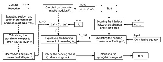
Figure 8.
Schematic diagram of spring-back prediction.
5. Spring-Back Prediction and Verification
5.1. FE Simulation
The FE simulation is one of the effective ways to obtain the engineering solution of the tube bending problem. Some bending characteristics, which are difficult to obtain in actual experiments such as the neutral layer shifting and the hidden defects of the double-layered tube, can be acquired from appropriate simulation post-processing. The FE simulation model of bimetallic tube CNC bending includes three parts i.e., material, geometry and physics. The material of the outer layer is 202 stainless steel and the material of the inner layer is Q235 carbon steel. This combination of materials considers both the external corrosion resistance and low cost. It may take effect in practical applications. The relevant parameters of the selected materials and the geometric parameters are listed in Table 4.
Table 4.
Material and geometry parameters of bimetallic tube.
At present, mature CNC bending usually adopts the form of plane rotation bending. The geometry model includes the bending die, the clamp die, the press die, the wiper die, and the bimetallic tube blank. The dies were set as rigid bodies while the tube was flexible.
On the physics side, the contact setting between double layers of the bimetallic tube is the key problem of simulation model construction, which directly affects the solution of coupling in the physical model. The composite forming process and bending process may lead to different contact conditions. On the platform of ANSYS Workbench, the contact between double layers of mechanical combination is mainly divided into bonded contact, frictional contact and existing gaps. If the combination is metallurgical, the material coupling between double layers should be considered and set further. In the model of Guo et al. [19], the contact was set as bonded. This means the contact surface of two layers has no normal separation or tangential movement during bending. Islam et al. [33] treated the combination of double layers as an interference fit. The sticking friction coefficient exists on the interface. In the hydro-bending of a double-layered tube, there is an initial installation gap between two layer of straight tube blanks. This paper focused on bimetallic tubes composited by mechanical combination. The interference fit was expressed by the friction coefficient 0.2. Other contacts between the outer tube and the dies were set as frictional contacts with the coefficient 0.1. The geometric model is shown in Figure 9. The gap between dies and the outer tube is 0.1 m while the clamping section does not exist any gap. The tube blank was bent by rotating the bending die and the clamp die together. The spring-back state can be acquired by rotating the bending die reversely. The bimetallic tube and contact faces were meshing by the sweep method and the hexahedral mesh was acquired. The element type was Solid186(3D20N). The static structural solver was adopted.
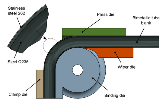
Figure 9.
Model of the bimetallic tube computer numerically controlled (CNC) bending.
5.2. CNC Bending Experiments of the Bimetallic Tube
According to the materials and size of the bi-layered tube above, the full-scale CNC bending experiments were carried out. The mechanical bonding strength of the bimetallic tube was selected to let the interlaminar friction coefficient close to 0.2. The King-Mazon PB50CNC tube bender (manufactured by King-Mazon Co., Ltd., Lishui, China) was used to bend the tubes and the HEXAGON 83 absolute arm was used to probe the tube angle. Figure 10 shows the bending equipment adopted (a) and the measuring instrument for tube bending angle (b) respectively. Figure 11 shows the test samples of stainless steel-carbon steel bimetallic tube after bending and spring-back.
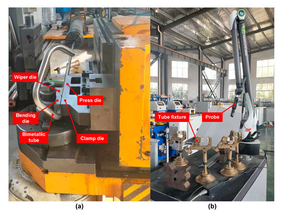
Figure 10.
CNC bending processing equipment for metallic tubes (a) and the measuring instrument (b).
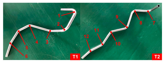
Figure 11.
Test samples of stainless steel-carbon steel bimetallic tube.
After angle measuring, the 90° bending section was cut along the direction of the bending plane. As is shown in Figure 12, there is no gap between the outer layer and the inner layer or wrinkling. It’s evident that the bending processes under all the angles are effective because 90° is the biggest bending angle and the degree of defect occurrence is proportional to the bending angle. To decrease the errors, two bimetallic tubes of the same size were bent in identical condition. The average of five measurements is listed in Table 5.
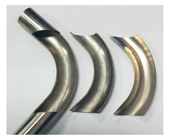
Figure 12.
Cutaway view of 90° bending section.
Table 5.
Experimental data.
6. Results and Comparison
6.1. Neutral Layer Shifting
Figure 13 shows the neutral layer shifting results from simulation experiment and RSM model prediction respectively. The trends of these two are basically consistent. The severe deformation of the thin-wall tube can account for the negative value of RSM model in this figure. Their relativity can be calculated as follow:
where and denote sets of the two results, and m denotes the number of experimental results as before and . In the same bending condition with the above actual experiments, the bimetallic tube bending is also simulated. Figure 14 shows the neutral layer shifting under different bending angles. The results come from RSM model prediction and simulation extraction respectively. Expect the 15°, under other bending angle, the relative errors of RSM model to simulation are less than 9.82%. It can be indicated that the RSM model works well and the neutral layer shifting calculated from the model is accurate enough. The 15° bending angle has not been contained in the experiment design because this angle is small, and its results may be non-representative. As a consequence, the relative error under 15° bending is 15.64% and greater than other relative errors.
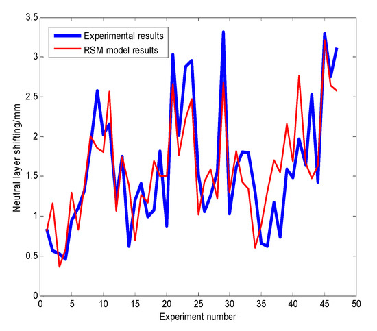
Figure 13.
Comparison of neutral layer shifting results.
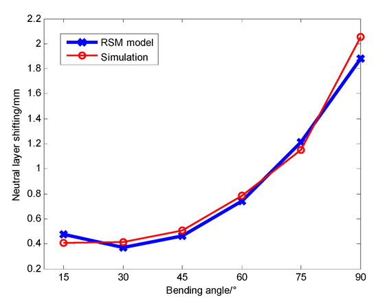
Figure 14.
Neutral layer shifting under 15~90° bending.
Though analysis of variance, in the factors mentioned above, layered thickness ratio has the greatest influence and interlaminar friction coefficient has the second greatest influence on the neutral layer shifting. Other factors affect the results more slightly comparatively. Diameter-thickness ratio, outer diameter, bending angle, and relative bending radius have sequentially reduced impacts on the neutral layer shifting. The response of the neutral layer shifting to layered thickness ratio and the interlaminar friction coefficient is illustrated in Figure 15a. The response of the neutral layer shifting to layered thickness ratio and diameter–thickness ratio is illustrated in Figure 15b.
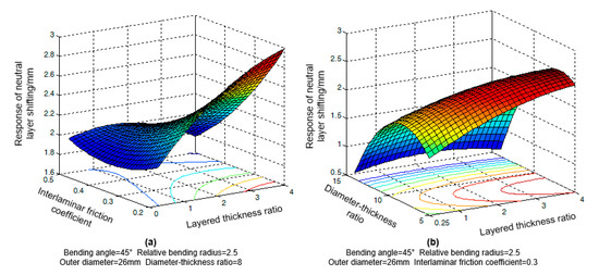
Figure 15.
Response value of neutral layer shifting to significant factors.
6.2. Spring-Back
Through the FE analysis, the stress distributions of bimetallic bending tubes under different bending angles were shown in Figure 16. In this figure, the uploading states were illustrated in (a1)~(a6) and the spring-back states illustrated in (b1)~(b6). The stress neutral layer displayed clearly on the cloud chart. The ultimate stress on the bimetallic tubes under the uploading process appears at the bending start. Meanwhile, the largest residual stress after unloading occurs near the neutral layer. There were some tiny shape defects on the cloud chart, such as wrinkling waves and point separation between double layers. Because it is hard to measure these tiny defects in the empirical experiments, they were neglected in this paper.
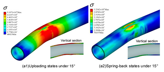
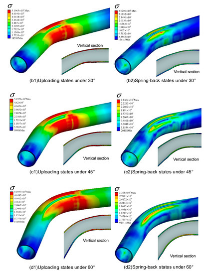
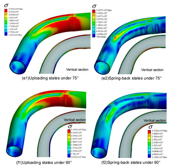
Figure 16.
Uploading and spring-back states under 15~90° bending: (a1) Uploading states under 15°; (a2) Spring-back states under 15°; (b1) Uploading states under 30°; (b2) Spring-back states under 30°; (c1) Uploading states under 45°; (c2) Spring-back states under 45°; (d1) Uploading states under 60°; (d2) Spring-back states under 60°; (e1) Uploading states under 75°; (e2) Spring-back states under 75°; (f1) Uploading states under 90°; (f2) Spring-back states under 90°.
Figure 17 illustrates the spring-back angles of bimetallic tubes under increasing bending angle. This figure contains four kinds of spring-back results. They are the spring-back angles from experiments, FE simulation analysis, theoretical calculation neglecting neutral layer shifting and theoretical calculation considering NLSE. In the calculation process, the interlaminar friction coefficient is 0.2 and the same as the simulation. While calculating the unloading moment, referring to E and Zhou [34], the cross-section takes the model that the short axis change rate of bending outside is 0.05, and the wall-thickness is invariable.
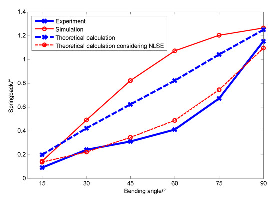
Figure 17.
Spring-back angles under 15~90° bending.
It can be found that the spring-back angles from FE analysis are almost greater than others. That is because the spring-back in the simulation environment can be affected by many special factors, such as the unloading method, meshing, contacts, friction between the tube and dies, the position of dies, etc. It is difficult to consider all these factors in the theoretical models. This may conduce to the difference between the results from FE analysis and theoretical models. The pure theoretical spring-back angles have a positive linear correlation with the bending angle. Compared with the theoretical results neglecting neutral layer shifting, the theoretical results considering NLSE are closer to the experimental results. Generally, the spring-back angle increases with the bending angle increasing. The angle differences between the theoretical results considering NLSE and experimental results are less than 0.0766°. Under 30~90° bending, the relative errors of theoretical spring-back angles to experimental spring-back angles are less than 18.68%. The relative errors between the forming angles after spring-back are less than 0.1258%. Under 15° bending, the largest error of the forming angles is 0.3159%. It is demonstrated that the accuracy of the theoretical model is acceptable.
To investigate the coupling between the two layers, the change of spring-back angles with the increasing of interlaminar friction coefficient is illustrated in Figure 18. The values of other factors are constant. It can be obvious from the diagram that the impact of interlaminar friction coefficient to bimetallic tubes’ spring-back is not monotonic. In the unloading spring-back process, the potential energy in the elastic deformation region of the bimetallic tube transfers to the kinetic energy and work caused by interlaminar friction. Even so, the final state of the bimetallic tube still exists some elastic potential energy. The layer whose spring-back trend is larger caused an extra elastic deformation on the other one layer. These can account for the monotonic phenomena. When the interlaminar friction coefficient is near 0.3~0.4, the spring-back angle is the largest. The spring-back angles from theory and FE analysis have the same trend. The simulation results are generally larger than the theoretical results by 0.0548°.
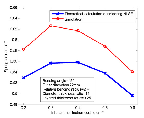
Figure 18.
Effect of interlaminar friction coefficient on the spring-back angle.
7. Conclusions
- Under the bending condition within 90°, the spring-back angle of the bimetallic tube is increased with the bending angle. This trend is the same as single-layered tubes. It indicates that the increase of plastic deformation degree with the increasing of bending angle does not matter for the spring-back of bimetallic tubes. The spring-back angle does not decrease with the increasing of the plastic deformation degree, and the bending angle is still the main effective factor of bimetallic tubes’ spring-back. If the neutral layer shifting is neglected, the theoretical spring-back angles of bimetallic tubes will increase linearly with the bending angle. The theoretical spring-back angles considering the NLSE model are smaller and closer to experimental results.
- The section strain of bimetallic tubes is continuous at the contact between layers. Therefore, the neutral layer shifting of bimetallic tubes can be described by the position of the coincident strain neutral layer. While the outer material is stainless steel and the inner material is carbon steel, the greatest effective factor of the bimetallic tubes’ neutral layer shifting is the layered thickness ratio. The effective secondary factor is the interlaminar friction coefficient. Generally, the larger the layered thickness ratio and the smaller the interlaminar friction coefficient, the larger the neutral layer shifting.
- When the interlaminar friction coefficient is below 0.3, the spring-back angle of bimetallic tube increase with the increase of the interlaminar friction coefficient. For those normal mechanical bonding bimetallic tubes, their interlaminar friction coefficients are less than 0.3 generally. In order to reduce the spring-back and improve the forming accuracy, suitable materials should be selected, and appropriate surface treatments can be done on the interface to reduce the friction coefficient.
Author Contributions
S.Z. and M.F. designed the simulations and experiments. M.F. proposed the spring-back method of bimetallic tubes and established the composite neutral layer model. M.F. and Z.W. performed the numerical simulations and the regression analysis. Y.L. performed the CNC tube bending experiments. M.F., Z.W., Y.L. and C.H. wrote the paper. All authors have read and agreed to the published version of the manuscript.
Funding
This work has been funded by the National Natural Science Foundation of China (51905476) and the Key R&D Program of Zhejiang Province (2019C05SAB51751).
Conflicts of Interest
The authors declare no conflict of interest.
References
- Yang, H.; Li, H.; Zhang, Z.; Zhan, M.; Liu, J.; Li, G. Advances and trends on tube bending forming technologies. Chin. J. Aeronaut. 2012, 25, 1–12. [Google Scholar] [CrossRef]
- Li, H.; Yang, H.; Zhang, Z.; Li, G.; Liu, N.; Welo, T. Multiple instability-constrained tube bending limits. J. Mater. Process. Technol. 2014, 214, 445–455. [Google Scholar] [CrossRef]
- Li, S.J.; Zhou, C.Y.; Li, J.; Pan, X.; He, X. Effect of bend angle on plastic limit loads of pipe bends under different load conditions. Int. J. Mech. Sci. 2017, 572–585. [Google Scholar] [CrossRef]
- Lapovok, R.; Ng, H.P.; Tomus, D.; Estrin, Y. Bimetallic copper–aluminium tube by severe plastic deformation. Scr. Mater. 2012, 66, 1081–1084. [Google Scholar] [CrossRef]
- Salehi, J.; Rezaeian, A.; Toroghinejad, M.R. Fabrication and characterization of a bimetallic Al/Cu tube using the tube sinking process. Int. J. Adv. Manuf. Technol. 2018, 96, 153–159. [Google Scholar] [CrossRef]
- Ganesh, P.; Kaul, R.; Mishra, S.; Bhargava, P.; Paul, C.; Singh, C.P.; Tiwari, P.; Oak, S.M.; Prasad, R.C. Laser rapid manufacturing of bi-metallic tube with Stellite-21 and austenitic stainless steel. T Indian I Metals 2009, 62, 169–174. [Google Scholar] [CrossRef]
- Chen, W.C.; Petersen, C. Corrosion performance of welded CRA-lined pipes for flowlines. SPE Prod. Eng. 1992, 7, 375–378. [Google Scholar] [CrossRef]
- Scharinger-Urschitz, G.; Walter, H.; Brier, J. Experimental investigation on bimetallic tube compositions for the use in latent heat thermal energy storage units. Energy Convers. Manag. 2016, 125, 368–378. [Google Scholar] [CrossRef]
- Wang, X.; Li, P.; Wang, R. Study on hydro-forming technology of manufacturing bimetallic CRA-lined pipe. Int. J. Mach. Tools Manuf. 2005, 45, 373–378. [Google Scholar] [CrossRef]
- Sun, C.; Liu, J.; Yao, X.; Huang, B.; Li, Y. Research on liquid impact forming technology of double-layered tubes. IOP Conf. Series: Earth Environ. Sci. 2018, 128, 012081. [Google Scholar] [CrossRef]
- Li, W.; Wen, Q.; Yang, X.; Wang, Y.; Gao, D.; Wang, W. Interface microstructure evolution and mechanical properties of Al/Cu bimetallic tubes fabricated by a novel friction-based welding technology. Mater. Des. 2017, 134, 383–393. [Google Scholar] [CrossRef]
- Li, H.; Shi, K.P.; Yang, H.; Tian, Y.L. Significance analysis of processing parameters on wall thinning in tube bending. Adv. Mater. Res. 2012, 622, 437–441. [Google Scholar] [CrossRef]
- Daxin, E.; Liu, Y.; Feng, H. Deformation analysis for the rotary draw bending process of circular tubes: Stress distribution and wall thinning. Steel Res. Int. 2010, 81, 1084–1088. [Google Scholar] [CrossRef]
- Huang, T.; Wang, K.; Zhan, M.; Guo, J.; Chen, X.; Chen, F.; Song, K. Wall thinning characteristics of Ti-3Al-2.5V tube in numerical control bending process. J. Shanghai Jiaotong Univ. 2019, 24, 647–653. [Google Scholar] [CrossRef]
- Liu, N.; Yang, H.; Li, H.; Tao, Z.; Hu, X. An imperfection-based perturbation method for plastic wrinkling prediction in tube bending under multi-die constraints. Int. J. Mech. Sci. 2015, 98, 178–194. [Google Scholar] [CrossRef]
- Yang, L.; Shi, S. Wrinkling analysis for rotary-draw bending of thin-walled tube filled with steel balls. Steel. Res. Int. 2012, 551–554. [Google Scholar]
- Li, H.; Yang, H.; Zhan, M.; Gu, R. A new method to accurately obtain wrinkling limit diagram in NC bending process of thin-walled tube with large diameter under different loading paths. J. Mater. Process. Technol. 2006, 177, 192–196. [Google Scholar] [CrossRef]
- Hasanpour, K.; Barati, M.; Amini, B.; Poursina, M. The effect of anisotropy on wrinkling of tube under rotary draw bending. J. Mech. Sci. Technol. 2013, 27, 783–792. [Google Scholar] [CrossRef]
- Guo, X.; Wei, W.; Xu, Y.; El-Aty, A.A.; Liu, H.; Wang, H.; Luo, X.; Tao, J. Wall thickness distribution of Cu–Al bimetallic tube based on free bending process. Int. J. Mech. Sci. 2019, 150, 12–19. [Google Scholar] [CrossRef]
- Wang, X.; Li, F. Analysis of wall thickness variation in the hydro-bending of a double-layered tube. Int. J. Adv. Manuf. Technol. 2015, 81, 67–72. [Google Scholar] [CrossRef]
- Gavriilidis, I.; Karamanos, S.A. Bending and buckling of internally-pressurized steel lined pipes. Ocean Eng. 2019, 171, 540–553. [Google Scholar] [CrossRef]
- Teng, B.G.; Hu, L.; Liu, G.; Yuan, S.J. Wrinkling behavior of hydro bending of carbon steel/Al-alloy bi-layered tubes. Trans. Nonferrous Met. Soc. China 2012, 22, s560–s565. [Google Scholar] [CrossRef]
- Zhan, M.; Wang, Y.; Yang, H.; Long, H. An analytic model for tube bending springback considering different parameter variations of Ti-alloy tubes. J. Mater. Process. Technol. 2016, 236, 123–137. [Google Scholar] [CrossRef]
- Zhang, Z.; Wu, J.; Guo, R.; Wang, M.; Li, F.; Guo, S.; Wang, Y.; Liu, W. A semi-analytical method for the springback prediction of thick-walled 3D tubes. Mater. Des. 2016, 99, 57–67. [Google Scholar] [CrossRef]
- Wu, J.; Zhang, Z.; Shang, Q.; Li, F.; Wang, Y.; Hui, Y.; Fan, H. A method for investigating the springback behavior of 3D tubes. Int. J. Mech. Sci. 2017, 131, 191–204. [Google Scholar] [CrossRef]
- Li, H.; Yang, H.; Tian, Y.; Li, G.; Wang, Z. Geometry-dependent springback behaviors of thin-walled tube upon cold bending. Sci. China Ser. E: Technol. Sci. 2012, 55, 3469–3482. [Google Scholar] [CrossRef]
- Song, F.; Yang, H.; Li, H.; Zhan, M.; Li, G. Springback prediction of thick-walled high-strength titanium tube bending. Chin. J. Aeronaut. 2013, 26, 1336–1345. [Google Scholar] [CrossRef]
- Dan, W.J.; Zhang, W. Springback angle and plastic elongation prediction of thin-walled tube bending by FEM. Appl. Mech. Mater. 2012, 152, 456–461. [Google Scholar] [CrossRef]
- Shayan, M.; Mohammadpour, M.; Malaki, M.; Ding, H. Springback analysis of two-layer strips in clad cold bimetal bending. Trans. Indian Inst. Met. 2014, 67, 851–859. [Google Scholar] [CrossRef]
- Liu, J.; Xue, W. Unconstrained bending and springback behaviors of aluminum-polymer sandwich sheets. Int. J. Adv. Manuf. Technol. 2016, 91, 1517–1529. [Google Scholar] [CrossRef]
- Liu, J.; Li, L. Springback behaviors of bi-layered non-homogeneous bellows in hydroforming. Int. J. Adv. Manuf. Technol. 2017, 93, 1605–1616. [Google Scholar] [CrossRef]
- Daxin, E.; Guo, X.; Ning, R. Analysis of strain neutral layer displacement in tube-bending process. Chin. J. Mech. Eng. 2009, 45, 307. [Google Scholar] [CrossRef]
- Islam, M.; Olabi, A.G.; Hashmi, M. Feasibility of multi-layered tubular components forming by hydroforming and finite element simulation. J. Mater. Process. Technol. 2006, 174, 394–398. [Google Scholar] [CrossRef]
- Xin, E.D.; Zhou, D. Metal Tube Bending: Theory and Forming Defects Analysis; Beijing University of Technology Press: Beijing, China, 2016. [Google Scholar]


© 2020 by the authors. Licensee MDPI, Basel, Switzerland. This article is an open access article distributed under the terms and conditions of the Creative Commons Attribution (CC BY) license (http://creativecommons.org/licenses/by/4.0/).