Evaluating Machine Learning Classification Using Sorted Missing Percentage Technique Based on Missing Data

Abstract

Missing data are common in industrial sensor readings owing to system updates and unequal radio-frequency periods. Existing methods addressing missing data through imputation may not always be appropriate. This study presented a sorted missing percentages technique for filtering attributes when building machine learning classification models using sensor readings with missing data. Signal detection theory was employed to evaluate the distinguishing ability of resulting models. To evaluate its performance, the proposed technique was applied to a publicly available air pressure system dataset, which then was used to build several classifiers. The experimental results indicated that the proposed technique allowed a logistic regression model to achieve the best accuracy score (99.56%) and a better distinguishing ability (response bias of 0.0013, adjusted response bias of 0.0044, and decision criterion of −1.8994) compared with the methods applied to the same dataset and reported in papers published between 2016 and 2019 March on binary classification, wherein attributes with more than 20% of missing data were filtered out. The proposed technique is suitable for industrial sensor data analysis and can be applied to the scenarios dealing with missing data owing to unequal radio-frequency periods or a system being updated with new fields.

1. Introduction

Industrial level sensors are employed as standalone devices (e.g., to measure temperature and humidity independently), packed modules (e.g., to measure temperature and humidity synchronously), or even bundled in target systems. With the rapid development of the Internet of Things, the production and procurement costs of sensors effectively satisfy the economic requirements of customers. In addition, multiple sensors can be configured in existing and single structures [1]. Daily collected data are useful for enterprises, particularly for meeting set objectives, i.e., preventive maintenance plans. Compared with sensors used in social sciences and medical fields, industrial sensors generate more missing data during data collection. The occurrences of missing data in industrial applications are primarily due to system updates and unequal radio-frequency periods, which are expected situations.

In real applications, determining the approaches of addressing missing data is a common challenge prior to implementing meaningful models for decisions. Generally, analysts determine possible reasons for missing data based on their industry background and work experience, and then take appropriate steps to address them. This study considers the following two general scenarios: data are missing completely at random or missing at random [2,3]. Appropriate strategies for dealing with these scenarios are to either ignore missing data or impute meaningful values [2,4]. However, it is difficult to establish whether data are missing with randomness when they are sourced from hundreds or even thousands of sensors. For example, Scania, the world’s leading provider of transport solutions, has proposed a viable maintenance plan based on budget constraints for their global customers [5,6]. Not all predefined data fields can be collected because some fields may not be permitted due to the purchased maintenance plan. In such circumstances, it is more appropriate to treat missing data as non-existing or of a separate type of natural event. Particularly, the constantly generated unstructured sensor data, which may likely contain many predictors to possible failures. Thus, it is a daunting task to collect, store, and analyze all such data [7]. Otherwise, missing data can be presented in both the training and test sets, only the training set, only the test set, or neither sets. To the best of our knowledge, the distribution consistency of training and test sets is not discussed frequently in the literature related to missing data manipulation.

Class imbalance is another factor that impacts the results of a classification model. Fernández et al. [8] stated that class imbalance hinders the performance of classifiers owing to their accuracy-oriented design, which typically results in the minority class being overlooked. Using a benchmark dataset from the KEEL (Knowledge Extraction based on Evolutionary Learning) repository, the authors proposed the imbalance ratio (IR) for identifying the degree of class imbalance (1.5 ≤ IR < 9: moderately imbalanced; IR ≥ 9: highly imbalanced). Class imbalance problems occur frequently in many applications in various fields, and there are two general approaches to deal with this problem that satisfy different requirements. One approach is to apply a resampling (under- or over-sampling) method to achieve a balance between the majority and minority classes. The other approach is to apply a weighting method assigning different weights to the majority and minority classes. Additionally, then, the examples from different classes are in equal status. Whichever approach is used, the original data distribution would change. Different combinations of the three factors (missing data, consistency of their distribution across the training and test sets, and class imbalance) can generate many different scenarios. Among them, the most common scenario is where classes are highly imbalanced, data are missing in both the training and test sets, and the assumption of consistent distribution between the training and test sets is not satisfied.

The empirical study data is a publicly available air pressure system (APS) dataset, initially presented at the Industrial Challenge 2016 at the 15th International Symposium on Intelligent Data Analysis (IDA) [9]. Our numerical analysis shows good results relative to several performance indicators, fewer misclassifications, and better distinguishing ability.

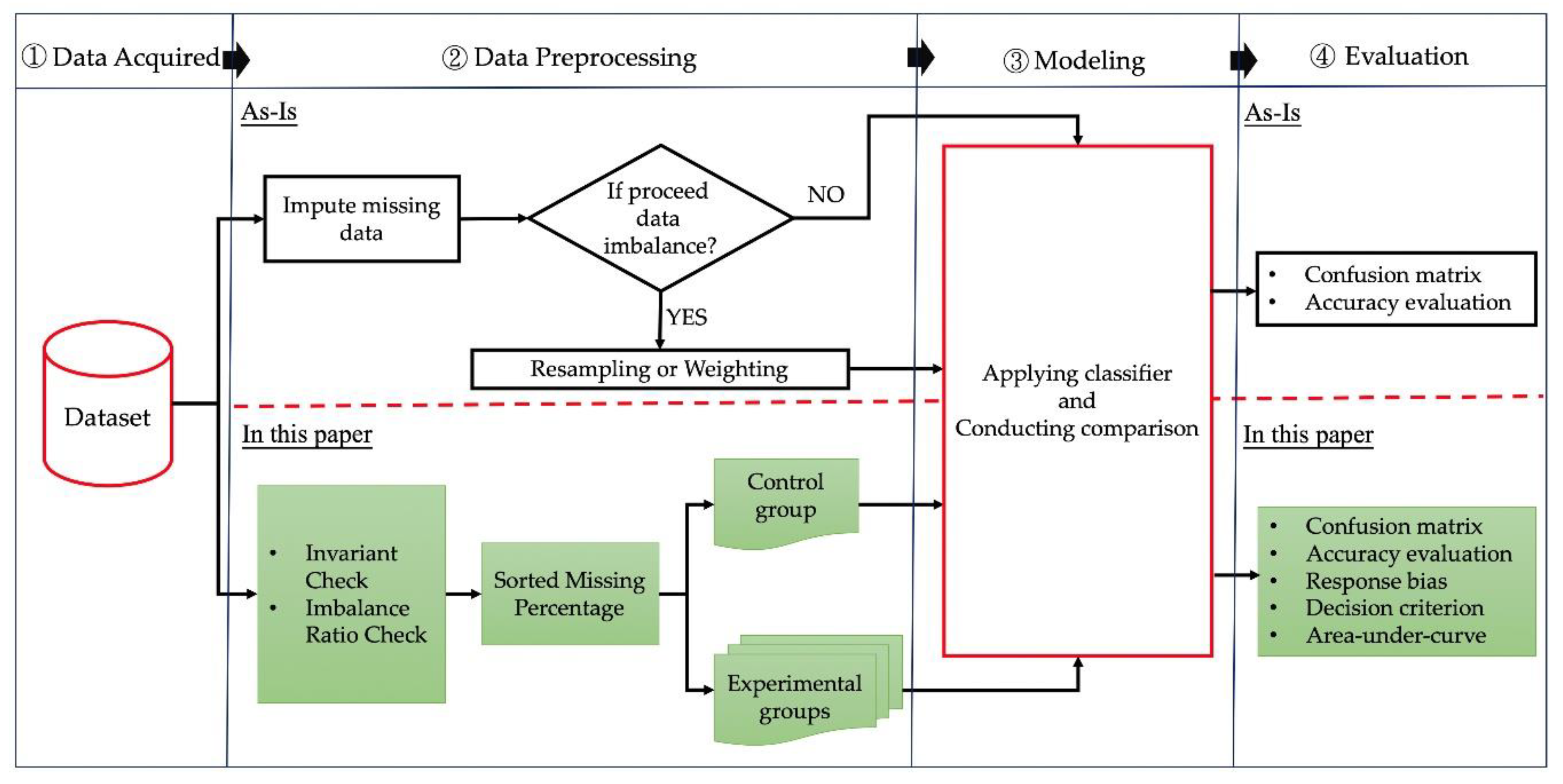
The rest of this paper is organized as follows. Section 2 introduces the proposed technique for addressing missing data. The numerical results of an empirical study are reported in Section 3. Section 4 discusses the results, while Section 5 concludes the paper.

2. Materials and Methods

2.1. Related Work

The APS dataset included two classes (NEG and POS). The calculated imbalance ratio was 59 in the training set and 41 in the test set. This set of public data was used for an empirical analysis of various topics. In terms of publication time, it can be divided into two scopes. Previous studies from 2016 to 2019 March [10,11,12,13,14,15,16] have used many dedicated methods of data imputation and machine learning algorithms to solve the high-class imbalance and missing data problems [17,18,19,20,21,22,23,24]. However, these studies have focused only on the training set. They have not considered whether the assumption of a consistent distribution of missing data across the training and test sets is satisfied. After 2019 March, a couple of innovative articles related to artificial intelligence applications and data generating are published. For example, the Sjöblom (2019) introduced genetic algorithms as an evolutionary strategy in statistical learning (the XGBoost) and then to automate the optimization procedures [25]. Škrlj, B. et al. (2020) employed a self-attention network to estimate the feature importance and then build the prediction models [26]. The APS data is one of the nine experimental datasets. About the limited data due to missing data, in contrast to existing data generation techniques. Ranasinghe and Parlikad (2019) proposed a methodology capable of generating new and realistic failure data samples [27].

In this paper, the proposed sorted missing percentages technique is for filtering attributes when building machine learning classification models using sensor readings with missing data. Signal detection theory (SDT) was then employed to evaluate the distinguishing ability of the resulting models. The numerical results were compared to the studies published from 2016 to 2019 March.

The proposed technique applied sorted missing percentages to filter attributes and then determined the control (CTRL) and experimental (EXP) attribute groups during the data preprocessing stage of the machine learning modeling pipeline.

Figure 1 summarizes the workflows for machine learning modeling applied in previous (As-Is) and current (in this paper) studies. The workflows include the following stages: data acquired, data preprocessing, modeling, and evaluation. In the evaluation step, we employed more indicators compared to the previous studies to evaluate the model performance and its distinguishing ability.

2.2. Sorted Missing Percentage and Recommended Steps

The concept of sorted missing percentages was proposed by Biteus and Lindgren [14], who applied a cutoff value of 10% in their study that was related to the APS data [9]. This study used 10% as a cutoff value to construct a control group of attributes. It then explored different cutoff values to construct experimental groups of attribute. Filtering can be called conservative if the percentage of missing data was greater than the cutoff value. For example, by applying a cutoff value of 20% or 30%, fewer attributes but more instances can be selected compared with that of the control group. In contrast, filtering can be called liberal if the percentage of missing data is less than the cutoff value. For example, by applying a cutoff value of 5%, more attributes but less instances can be selected compared with that of the control group.

Note that this method does not alter the original data. Furthermore, the included instances can be used more flexibly when the maximum attribute space is established under different filtering criteria. This can be considered an advantage because, under the premise of the same maximum attribute space, the assumption of a consistent distribution between the training and test sets can be satisfied. Through comparison, it was established that the attribute space of the group producing the best model performance is also the best configurable attribute space for the considered dataset. The recommended steps for implementing the sorted missing percentage method for the groups can be summarized as follows.

• Step 1: Sort attributes in descending order of missing percentages.
• Step 2: Set a cutoff value of 10% and select all attributes with less than that 10% of missing values into the control group.
• Step 3: Set different missing percentages as thresholds and use them to define the experimental groups.
• Step 4: Compare the control and experimental groups. Select the group that yields the best model performance and define the best configurable attribute space.

2.3. Machine Learning Classifiers

This study used five classifiers, and these classifiers are the most widely used and the most mature algorithms currently. Each classifier has its own characteristics and different limitations with respect to its implementation. According to the prediction target and computational approach, all of these classifiers belong to binary (negative or positive) and discriminative classifiers. Due to the contents of outcomes, logistic regression (LR) is a type of probabilistic classifier, and the other four classifiers are deterministic classifiers. If we focus on attribute combinations and the learning process, LR and support vector machines (SVM) can be considered linear and global classifiers. In contrast, the k-nearest neighbors, random forest, and stochastic gradient boosting trees are nonlinear, iterative computing, and local classifiers, respectively [28]. To optimally interpret the provided data, the final classifier should be selected from a list of alternatives, and each must provide consistent model performance for both the training set (for modeling) and test set (for verification). A classifier is determined to be the best if it provides the best model performance and best distinguishing ability.

2.3.1. Logistic Regression (LR)

LR [29,30,31] is based on the regression model and frequently used for binary classification problems. For example, the negative class is assigned with label 0, whereas the positive class is assigned with label 1. The general form $\pi \left(x\right)$ and its logit transformation form $g\left(x\right)$ are given as follows:

$$\pi \left(x\right)=\pi \left(x_1, x_2,\dots , x_n\right), \pi \in \left\{0,1\right\}$$

$$g\left(x\right)=\ln \left[\frac{\pi \left(x\right)}{1-\pi \left(x\right)}\right]={\beta }_0+{\beta }_1{x}_1+{\beta }_2{x}_2+\dots +{\beta }_n{x}_n,$$

where $\left(x_{1, }{x}_{2, }\dots , x_n\right)$ is the vector of predictors and ${\beta }_i\left(i=1,2,\dots , n\right)$ are the regression coefficients of the predictors. Here, the output class labels were calculated as the logit-transformed probabilities. If the probability is close to 1, then the positive class is assigned.

2.3.2. Support Vector Machine (SVM)

SVMs [18,29,31,32,33,34] are based on the concept of building decision planes to define decision boundaries. The decision plane is a hyperplane that separates examples into the most likely categories with the maximum distance between them. For a binary classification task, the general form $Y$ and objective function $g\left(Y\right)$ are given as follows:

$$Y=\left\{y_i\right\}, y_i\in \pm 1, i=1, 2,\dots , n$$

$$g\left(Y\right)=\min \frac{1}{2}{\overline{w}}^T\overline{w}+C{\displaystyle \sum }_{i=1}^n{\phi }_i,$$

$$constrain to y_i\left(w^T\theta \left(x_i\right)+b\right)\ge 1-{\phi }_i, and {\phi }_i\ge 0, i=1, 2,\dots , n,$$

where $C$ is the capacity constant, $w$ is the vector of coefficients, $\phi$ is the slack variable, and $b$ is a constant used to handle non-separable data (i.e., inputs). The index $i$ labels the $n$ training examples, and the kernel $\theta$ is used to transform data from the input to the feature space. Here, larger $C$ values represent a higher degree of error penalization. When using an SVM, it is important to select and configure parameter $C$ appropriately to avoid overfitting.

2.3.3. k-Nearest Neighbors (k-NNs)

k-nearest neighbor (k-NN) [10,16,29,31,32,35] is a memory-based reasoning model (also referred to as instance-based learning) that includes a set of known examples, and the outcomes are known. Given a new example (i.e., the query point), the task is to classify the outcome through its k neighbors based on the selected distance metric, and the outcome is selected based on the majority votes (bagging) from the k neighbors. A small k value leads to large variance in predictions, whereas a large k value may lead to a high degree of model bias. For binary classification problems, the typical distance weighting $W$ is formed as follows:

$$W\left(x, p_i\right)=\frac{\exp \left(-D\left(x, p_i\right)\right)}{{\sum }_{i=1}^k\exp (-D\left(x, p_i\right))}, i=1, 2,\dots , k$$

$${\sum }_{i=1}^{k}W\left(x_{new}, x_i\right)=1,$$

where $x$ and $p$ are the query point and a case from the example sample, respectively, and $D\left(x, p_i\right)$ is the distance between the query point $x$ and case $p_i$ of the example sample. An optimal $k$ value is estimated using the cross-validation technique, which achieves an appropriate compromise between variance and bias, and avoids overfitting. The weighted distance between new query points $x_{new}$ in $k$-fold cross-validation is summed up to 1.

2.3.4. Stochastic Gradient Boosting Trees (GBTs)

A gradient boosting tree (GBT) [11,19,29,31,36,37] is an ensemble learning algorithm that includes a set of classifiers based on weighted examples. Here, the classifiers are built sequentially, and every misclassified example is labeled to minimize the target loss function. The general form $y_E^{n+1}$ of $a$ is given as follows:

$$y_E={\displaystyle \sum }_i{a}_i{f}_i\left(\overline{x}\right), i=1, 2,\dots$$

$$y_E^{n+1}=y_E+a_{n+1}{f}_{n+1}\left(\overline{x}\right)$$

$$y_E^{n+1}=y_E+a_{n+1}{\displaystyle \sum }_i\nabla L\left(y_{T_i},y_{E_i}\right)$$

where $y_E$ is the outcome of the ensemble, $f_i\left(x\right)$ is the function of the weak learners, $\nabla L$ is the loss function, and $y_{T_i}$ is the target class. With the GBT approach, several characteristics should be considered carefully, e.g., all involved classifiers are weak learners, normalization of examples is required before constructing the classifier, and overfitting can occur easily.

2.3.5. Random Forests (RFs)

Random forest (RF) [12,13,29,31,38] is an ensemble learning algorithm that involves a collection of decision trees (i.e., classifiers). The decision trees are independent identically distributed random vectors. In addition, the final selected tree is that with the most votes (bagging). The general form $DF$ and voting criteria $dDF\left(x\right)$ are given as follows:

$$DF=\left\{d_j:X\to \left\{1, 2, \dots , g\right\}\right\}, j=1, 2,\dots , J, J\ge 2$$

$$dDF\left(x\right)=arg\underset{c}{\min }{N}_c\left(x\right), c\in \left\{1, 2,\dots , g\right\}, N_c\left(x\right)=\#\left\{j:d_j\left(x\right)=c\right\},$$

where $d_j$ is the jth generated tree, $c$ is the decision class, and $N_c\left(x\right)$ is the number of votes for classification of sample $x\in X$ to class $c$.

2.4. Indicators for Model Performance

Accuracy, F-measure, and the Matthews correlation coefficient (MCC) [39] are commonly used to explain the model’s performance. The receiver operating characteristics (ROCs) curve is a two-dimensional graph presenting the relative tradeoff between true-positives on the Y-axis and false-positives on the X-axis [40]. The area under the curve (AUC) is a metric that summarizes the ROC curve [31]. The ROC curve and calculated AUC were used to visualize the predictive accuracy of the selected model. Furthermore, the criteria adopted in SDT [41,42] were used in this paper. SDT is more commonly used in psychophysics and psychology studies and is applied to various tasks, including detection, identification, recognition, and classification. Regardless of the task, the initial focus in these studies is on how to effectively analyze decision-making under uncertainty and bias, i.e., the model’s performance. The secondary focuses in SDT are determining how much information is obtained during decision-making and whether the obtained information is useful and applicable, i.e., the model’s distinguishing ability.

In SDT, β is defined as the ratio of neural activity produced by signal and noise; it is used to compute the response bias. ${\beta }_{opt}$ is the adjustment of $\beta$ used to detect changes in the signal and noise probabilities. ${\beta }_{opt,payoff}$ is involved with additional information such as the reward for correct events (Value) and the penalty for incorrect events (Cost).

$X_c$ is the decision criterion serving as a useful indicator reflecting a criterion shift. An $X_c$ value close to 0 indicates an unbiased decision. In other words, all the information was fully used during the decision-making process. A positive $X_c$ represents a type of liberal decision-making, which is also interpreted as information is overused. A negative $X_c$ indicates conservative decision-making, where information is filtered to reduce the risk of mistakes.

$$\beta =\frac{p\left(X|S\right)}{p\left(X|N\right)}=C\times d^{\prime }$$

$${\beta }_{opt}=\frac{P\left(N\right)}{P\left(S\right)}=\frac{count \left\{FP+FN\right\}}{count \left\{TP+TN\right\}}$$

$${\beta }_{opt, payoff}={\beta }_{opt}\times \frac{Value\left(TN\right)+Cost\left(FP\right)}{Value\left(TP\right)+Cost\left(FN\right)}$$

$$X_c=-\frac{z\left(TP\right)+z\left(FP\right)}{2},$$

where $X$ is the decision variable of binary classification for either $S$ (signal) or $N$ (noise); $C$ is the criterion that $X$ is presented, $d^{\prime }$ is the distance of the midways between the signal and noise distributions, $Value$ is a reward for events that are correctly classified, and $Cost$ is a penalty for events that are misclassified. True Negative ($TN$), False Positive ($FP$), True Positive ($TP$), and False Negative ($FN$) are the abbreviations of true-negative, false-positive, true-positive, and false-negative, respectively. $z\left(TP\right)$ is the z-distribution transformed values of the true-positive events, and is the z-distribution transformed values of the false-positive events.

3. Numerical Analysis

3.1. Dataset

The dataset used in this paper was initially provided by Scania CV AB (Sweden). The data were extracted from historical operational data, and included information based on on-board sensors showing how each truck has been used on average. The target system was the APS generating pressurized air, which is used in various truck functions such as braking and gear changing. There were 171 attributes: 100 single numerical counters and seven histograms with 10 bins each, and one class label. The attributes were categorized as a class and anonymized operational data. The operational data have an identifier and a bin id (Identifier_Bin). For example, attribute aa_000 was collected from class a, the operational identifier was aa, and the bin id was 000.

The dataset was divided into training and test sets by Scania experts (60,000 training examples and 16,000 test examples). The class label could be either POS or NEG, wherein POS indicates detected failures related to a specific APS system component and NEG indicates failures not related to any of the APS system components.

3.2. Data Profiling and Filtering

In this paper, the control and experimental attribute groups were defined for modeling and comparison (Figure 1).

Table 1. Invariant attribute assessment of the selected attribute cd_000.

Attribute	Valid N	#Missing	Mean	Median	Mode	Minimum	Maximum
cd_000	59,234	676 (1.13%)	1,209,600	1,209,600	1,209,600	1,209,600	1,209,600

lists selected results of the invariant check on attribute cd_000, representing class c, operational identifier cd, and bin id 000. As shown, attribute cd_000 had the same value for the mean, median, and mode, as well as the minimum and maximum values, which implies all valid data were the same. Therefore, this attribute should be removed from the list of attributes for predictive modeling. Including invariant attributes would only increase the computational cost.

Table 2. Number of instances of each class in the training and test sets.

CLASS	Training	Test
NEG	59,000	15,625
POS	1000	375
IR = NEG/POS	59.0	41.7

presents the overall IR check results based on the class label in the training and test sets. The calculated IRs of NEG to POS in the training and test sets were 59.0 and 41.7, respectively, which satisfies the definition of high class imbalance.

The IR is also a quick way of determining whether the training and test sets are consistently distributed for the given attributes. First of all, the examples of the attributes are labeled as VALID if they comprise real values. If the examples are shown as blank cells, they will be labeled as N/A. It is assumed that if the IR of individual attributes falls within a specified range centered on the overall IR, the assumption of a consistent distribution between the training and test sets was valid. Furthermore, 2 × 2 cross-tabulation was conducted. The calculated Chi-square results would clarify if the missing data behavior of the attributes was homogenous between NEG and POS classes disregarding whether the examples were from the training or test set. After performing IR checks on all attributes, the training set IR values were ranged between 55 and 61, whereas the test set values ranged between 39 and 43, with a single exception for the attribute ac_000. The ac_000 data was from the class a, the operational identifier was ac, and the bin id was 000. As shown in

Table 3. The imbalance ratio (IR) check and Chi-square test for attribute ac_000.

CLASS	Training	Test
NEG	56,127	14,878
POS	538	196
IR = NEG/POS	104.3	75.9
Pearson Chi-square	3199.883 (p-values = 0.0000)	1239.109 (p-values = 0.0000)
Maximum-Likelihood Chi-square	1406.807 (p-values = 0.0000)	555.167 (p-values = 0.0000)

, the calculated IRs for the training and test sets were 104.3 and 75.9, which were larger than the overall IRs of 59.0 and 41.7, respectively. The calculated Pearson Chi-square and maximum-likelihood Chi-square results (CLASS × ac_000) indicated statistical significance (p-values were both 0.0000). For these findings, it is recommended to remove attribute ac_000 from the list of predictive modeling attributes.

For the APS dataset, Biteus and Lindgren [14] recommended removing attributes with over 10% missing data; however, they do not explain why the criterion for filtering attributes was set to 10%. Following this concept, we created bins by the sorted missing percentages, namely, >30%, 20–30%, 10–20%, and 5–10%. Figure 2 shows the bar chart presenting the bins by different missing percentages.

Table 4. Contained attributes by sorted missing percentages.

% Missing	Attributes Contained in Training Set	Attributes Contained in Test Set	# Attributes
>30%	br_000, bq_000, bp_000, bo_000, ab_000, cr_000, bn_000, bm_000, bl_000, bk_000	br_000, bq_000, bp_000, bo_000, ab_000, cr_000, bn_000, bm_000, bl_000, bk_000	10
20–30%	ad_000, cf_000, cg_000, ch_000, co_000, ct_000, cu_000, cv_000, cx_000, cy_000, cz_000, da_000, db_000, dc_000	ad_000, cf_000, cg_000, ch_000, co_000, ct_000, cu_000, cv_000, cx_000, cy_000, cz_000, da_000, db_000, dc_000	14
10–20%	ec_00, cm_000, cl_000, ed_000	ec_00, cm_000, cl_000, ed_000	4
5–10%	ak_000, ca_000, dm_000, df_000, dg_000, dh_000, dl_000, dj_000, dk_000, eb_000, di_000, bx_000, cc_000	ca_000, ak_000, df_000, dg_000, dh_000, di_000, dj_000, dk_000, dl_000, dm_000, eb_000, bx_000, cc_000	13

shows the details for the contained attributes in each bin. As shown, the first three bins had the same attributes and sorting results for both the training and test sets. The fourth bin, 5–10%, had the same attributes but different sorting results.

According to the results in Table 4, the cumulative missing percentages were further used to define the control (CTRL) and experimental groups (EXP1, EXP2, and EXP3). After removing the attributes with more than 10% missing, the remaining 70 attributes were assigned to a bin and defined as a control group (CTRL). The missing percentage of attributes contained in EXP1 was less than 30% (contains 88 attributes), in EXP2 was less than 20% (74 attributes), and in EXP3 was less than 5% (57 attributes).

3.3. Comparison between the Control and Experimental Groups

Table 5. Performance results of the five considered classifiers for the control and experimental attribute groups over training and test sets.

Group	Classifier	Training Set (for Modeling)			Test Set (for Validation)
		Accuracy	F-Measure	MCC	Accuracy	F-Measure	MCC
CTRL	LR	99.58%	66.57%	67.45%	99.40%	66.67%	68.18%
	SVM	99.42%	37.80%	46.85%	99.15%	38.81%	47.93%
	k-NN	99.66%	72.04%	73.90%	99.26%	55.23%	58.41%
	GBT	98.91%	58.89%	60.53%	98.44%	55.36%	58.22%
	FR	98.33%	0.00%	0.00%	97.66%	0.00%	0.00%
EXP1	LR	99.82%	76.88%	77.57%	99.69%	67.29%	68.23%
	SVM	99.66%	38.98%	49.12%	99.60%	44.44%	53.34%
	k-NN	99.76%	65.51%	69.15%	99.63%	53.93%	59.17%
	GBT	98.94%	61.68%	62.56%	98.58%	59.49%	61.37%
	FR	98.33%	0.00%	0.00%	97.66%	0.00%	0.00%
EXP2	LR	99.68%	72.60%	73.44%	99.56%	73.24%	74.30%
	SVM	99.49%	41.43%	49.74%	99.28%	42.24%	51.00%
	k-NN	99.73%	76.23%	77.47%	99.44%	63.64%	65.91%
	GBT	98.93%	60.48%	61.65%	98.51%	58.86%	60.89%
	FR	98.93%	0.00%	0.00%	97.66%	0.00%	0.00%
EXP3	LR	99.29%	59.47%	60.61%	99.08%	62.09%	63.23%
	SVM	99.08%	25.86%	36.98%	98.79%	31.18%	42.71%
	k-NN	99.32%	59.01%	61.25%	98.89%	48.45%	51.91%
	GBT	98.86%	56.15%	58.04%	98.41%	54.64%	57.45%
	FR	98.33%	0.00%	0.00%	97.66%	0.00%	0.00%

lists the results of comparing the control and experimental attribute groups over that of the training and test sets. During the modeling phase using the training set, k-NN performed best in CTRL (99.66%), EXP2 (99.73%), and EXP3 (99.32%). LR was best in EXP1 (99.82%); however, it was second best in other groups. During the validation phase using the test set, LR showed the best results in all groups, and k-NN was second best. Thus, in addition to LR, k-NN could be considered as a suitable classifier for the APS dataset. Considering the scores obtained for accuracy, F-measure, and MCC, the combination of EXP2 and LR outperformed the other attribute groups and classifiers.

The stability of a prediction model must be considered for practical applications. Thus, k-NN can be considered as a potential candidate. If LR failed on the prediction or underperformed, then k-NN can be replaced. To get further insights into the models’ performance, decile-wise lift charts were employed to demonstrate the level of the prediction capability that can be produced by examples fed into the trained model. If few examples can produce a high prediction capability, then the calculated lift value is regarded to be high. Figure 3 shows the decile-wise lift charts to demonstrate how LR and k-NN perform by sample size (represented in percentages).

It can be noticed from Figure 3a that both LR and k-NN performed well when predicting the NEG class label. After inputting 80% of the examples of the test set, the performance of both the LR and k-NN models decreased. For the POS label, it can be noted from Figure 3b that the validation performance of LR was better than the k-NN in the first 10% of the test examples. While increasing test examples to 20% and up to 80%, the validation performance of k-NN was more stable because the calculated lift values were greater than 1.000. The valid test examples of EXP2 were 12,885 and 10% were approximated as 1289 (=12,885 × 10%). In other words, LR performed well for both the NEG and POS class labels only if the applied sample size was not larger than 1289. Otherwise, k-NN should be used instead of LR to predict either NEG or POS examples.

Table 6. Summary of $\beta$ and $X_c$ values for the selected LR model, for control and experimental groups.

	Training Set (for Modeling)				Test Set (for Validation)
Group	$\mathit{\beta }$	${\mathit{\beta }}_{\mathit{o}\mathit{p}\mathit{t}}$	${\mathit{\beta }}_{\mathit{o}\mathit{p}\mathit{t},\mathit{p}\mathit{a}\mathit{y}\mathit{o}\mathit{f}\mathit{f}}$	${\mathit{X}}_{\mathit{c}}$	$\mathit{\beta }$	${\mathit{\beta }}_{\mathit{o}\mathit{p}\mathit{t}}$	${\mathit{\beta }}_{\mathit{o}\mathit{p}\mathit{t},\mathit{p}\mathit{a}\mathit{y}\mathit{o}\mathit{f}\mathit{f}}$	${\mathit{X}}_{\mathit{c}}$
CTRL	0.0038	0.0042	0.0024	−1.7101	0.0049	0.0060	0.0019	−1.6587
EXP1	0.0003	0.0018	0.0004	−2.1413	0.0026	0.0031	0.0021	−1.7731
EXP2	0.0011	0.0032	0.0009	−1.9241	0.0013	0.0044	0.0007	−1.8992
EXP3	0.0152	0.0071	0.0056	−1.4396	0.0142	0.0093	0.0039	−1.4646

lists $\beta$ and $X_c$ values obtained for the LR model to demonstrate which of the considered attribute groups provides more stable results. All the $\beta$ values were very close to zero, which means that the control and experimental groups both returned an unbiased outcome. In addition, all calculated $X_c$ values were negative, which means these unbiased outcomes reflect conservative decision-making. Although the $\beta$ value was the smallest for EXP1 (0.0003) in the training set, it was eight times bigger for this group (0.0026) in the test set. EXP2 had the second smallest $\beta$ value (0.0011) in the training set and the smallest in the test set (0.0013). The small difference between these two values proved again that the LR model could deliver better classification results for EXP2 than for the other groups.

4. Discussion

The APS dataset was used as an empirical study on various topics related to classic machine learning; we reviewed some of those published between 2016 and 2019 March. Costa et al. [10] applied mean imputation and the Soft-Impute algorithm to handle missing data and concluded that RF was the best classifier owing to the highest cost-wise ratio of 92.56%, where the FP and FN rates were 3.74% and 3.70%, respectively. Cerquerira et al. [11] removed attributes with over 50% missing data, conducted metafeature engineering to generate new attributes, implemented Synthetic Minority Oversampling Technique (SMOTE) to replace the removed examples, and then concluded that XGBoost with meta-features yielded the lowest average cost and deviance. Condek et al. [12] applied median imputation address missing data and concluded that RF can be used as a cost function providing better results than the naïve approaches of checking every truck or no truck until failure. Ozan et al. [13] introduced an optimized k-NN approach to handle missing values and created a tailored k-NN model using a specified HEIM distance. Biteus and Lindgren [14] removed attributes with more than 10% missing values and applied mean imputation to the remaining attributes. They evaluated various classifiers, including RF, SVM, and k-NN, and selected RF, which returned an accuracy score of 0.99.

Rafsunjani et al. [15] used five imputation techniques, including expectation-maximization, mean imputation, Soft-Impute, Multivariate Imputation by Chained Equation (MICE), and iterative singular value decomposition, and applied five classifiers, including naïve Bayes (NB), k-NN, SVM, RF, and GBT. They concluded that NB performs better on the actual and imbalanced dataset; however, RF performed better on the balanced dataset after applying an under-sampling method. In addition, the mean imputation was identified as the best method for imputing missing values. However, if the primary concern is the FP rate rather than accuracy, then Soft-Impute was shown to outperform the other imputation techniques and NB was demonstrated to have the best performance compared to the other classifiers. Jose and Gopakumar [16] employed a k-NN algorithm for missing data imputation, implemented an improved RF algorithm to reduce both the FP and FN misclassification rates, and demonstrated competitive results in terms of precision, F-measure, and MCC.

Table 7. Comparison of the proposed approach to methods reported in previous studies based on accuracy, F-measure, and Matthews correlation coefficient (MCC) over the test set.

Source	MD Imputation	Classifier	Accuracy	F-Measure	MCC
Costa and Nascimento (2016)	Mean, Soft Impute	RF	96.56%	57.05%	61.55%
Condek, Hafner, and Sampson (2016)	Median	RF	96.86%	59.12%	63.08%
Sumeet et al. (2016)	N/A	N/A	97.42%	63.55%	66.55%
Biteus and Lindgren (2017)	Mean	RF	96.53%	56.67%	61.09%
Rafsunjani et al. (2019)—Under-sampling	MICE	RF	94.79%	46.81%	53.32%
Rafsunjani et al. (2019)—Actual Data	Interactive SVD	NB	96.39%	53.76%	57.32%
Jose and Gopakumar (2019)	k-NN (k = 33)	Modified RF	97.29%	62.46%	65.70%
EXP2-LR (this paper)	No Impute	LR	99.56%	73.24%	74.30%

compares the results achieved in this paper for the EXP2-LR combination with those of the previous studies in terms of accuracy, F-measure, and MCC.

The previous studies included for the comparison applied imputation techniques directly to missing data in the training set; however, the process is not discussed and assumptions related to the consistency of the training and test datasets were not provided. In addition, the training and test sets were not evaluated after applying imputation to determine if they satisfy the assumption of a consistent distribution. It can be noticed from Table 7 that the recommended model, EXP2-LR, had the best accuracy (99.56%), F-measure (73.24%), and MCC (74.30%) results.

Table 8. Comparison of the proposed approach to methods reported in previous studies based on $\beta$ values and X_c over the test set.

Source	$\mathit{\beta }$	${\mathit{\beta }}_{\mathit{o}\mathit{p}\mathit{t}}$	${\mathit{\beta }}_{\mathit{o}\mathit{p}\mathit{t},\mathit{p}\mathit{a}\mathit{y}\mathit{o}\mathit{f}\mathit{f}}$	${\mathit{X}}_{\mathit{c}}$
Costa and Nascimento (2016)	0.0000	0.0357	0.0001	−2.8854
Condek, Hafner, and Sampson (2016)	0.0000	0.0324	0.0001	−2.7828
Sumeet G., et al. (2016)	0.0000	0.0265	0.0001	−2.7267
Biteus and Lindgren (2017)	0.0000	0.0359	0.0001	−2.7597
Rafsunjani, S., et al. (2019)—Under-sampled	0.0000	0.0550	0.0002	−2.8358
Rafsunjani, S., et al. (2019)—Actual Data	0.0013	0.0375	0.0013	−2.1683
Jose, C., and Gopakumar, G (2019)	0.0000	0.0279	0.0001	−2.7469
EXP2-LR (in this paper)	0.0013	0.0044	0.0007	−1.8992

compares the results achieved in this paper for the EXP2-LR combination with those of the previous studies in terms of $\beta$ and $X_c$ values, which indicate the effectiveness of the selected classifiers for binary classification. It can be noticed from the table that, the previously reported methods all provided unbiased outcomes ($\beta$ values were close to zero) and conservative decision-making ($X_c$ is negative). While the $\beta$ values of the previous methods indicate perfect unbiased results, the related ${\beta }_{opt}$ values were high, which means that the validated results were not sufficiently generalized. In other words, the previous studies pay more attention to examples with the NEG class label than those with the POS class label. They may be able to minimize the FN score but at the cost of increasing FP scores. Furthermore, the $X_c$ values of all previous methods were smaller (i.e., bigger negative numbers) than that of the EXP2-LR model, which indicates that previous methods provided more conservative decisions. These results demonstrated that the EXP2-LR model recommended in this paper achieved the best performance in the considered binary classification task.

Two further findings were discussed here. First, according to the SDT, when the $\beta$ values were close to zero, the selected model was implemented with few biases. This characteristic is adjusted by applying additional weights such as penalties and rewards (usually are predefined by experienced experts). Previous studies published between 2016 and 2019 March implemented various imputation techniques; however, these manipulations do not improve the recognition ability of the reported models. In contrast, adding weight values might cause more conservative decision-making.

The second finding is about data representativeness after resampling. An inappropriate resampling method can lead to new problems, e.g., insufficient fitting, even if it improves the original class imbalance. Rafsunjani et al. [15] compared actual data to under-sampled data. As shown in Table 8, the $\beta$ value calculated for the under-sampled data was more unbiased ($\beta$ was 0.0000, i.e., perfectly unbiased) than that calculated for the actual data ($\beta$ was 0.0013, i.e., very unbiased). However, the ${\beta }_{opt}$ and $X_c$ values calculated for the under-sampled data (0.0550 and −2.8358, respectively) were farther from zero than those for the actual data (0.0375 and −2.1683, respectively), which means the under-sampled data were more conservative. Regardless of the resampling method used (under- or over-sampling), the recommendation for the subsequent processing on the transformed data was to first check the consistent distribution assumption.

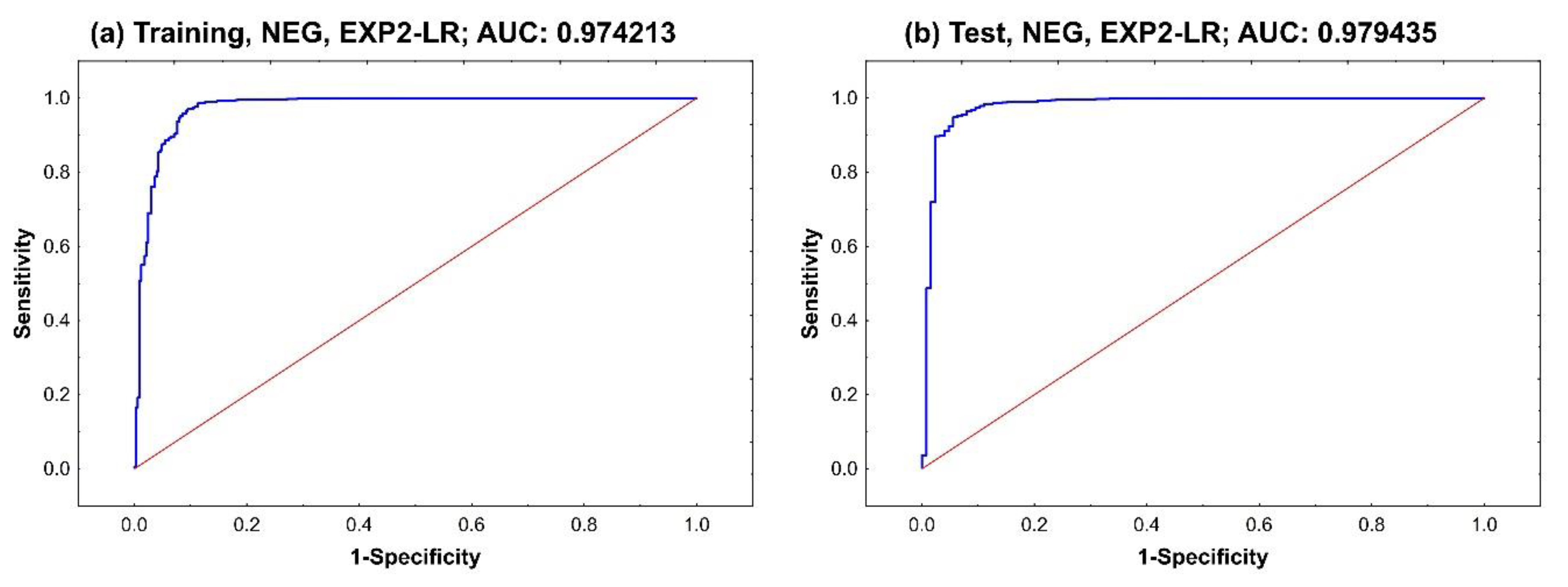
Under such circumstances, advanced metrics such the ROC curve and AUC should be used to provide a wider understanding of the model’s performance over the training and test sets, i.e., during modeling and validation. Figure 4 shows the ROC curves for the selected EXP2-LR model considering the NEG class label, separately for the training and test sets. The calculated AUC values for the training and test sets were 0.974213 and 0.979435, respectively. A high AUC value means that the trained model returns a great result during the validation phase. It also means that the selected model is applicable. The trends of the two NEG curves were similar. Both curves quickly reached the top, almost fully sensitive, when the 1-specificity value was close to 0.1; 1-specificity is also known as the FP rate and represents the probability of a Type I error or false alarm event. In addition, the NEG curves for the test set were steeper than those for the training set.

Figure 5 shows the ROC curves and AUC values for the EXP2-LR model considering the POS class label, separately for the training and test sets. Compared to the curves for the NEG class label, the curves for the POS class label rose more quickly at the beginning until 1-specificity was reached at a value of 0.2. The POS curves go downward when the 1-specificity value was between 0.02 and 0.5. After that, the curves tended to flatten.

Based on the above results, it was proved that the selected EXP2-LR model was outperformed on the APS data than other machine learning models created from the previous articles. Further, under the data conditions proposed as EXP2, as a candidate model, k-NN also can generate a higher ACC (99.44%) and F-measure (63.64%), and a bit weaker MCC (65.91%) than previous models (Table 5 and Table 7). When the existence of missing data is a kind of reasonable behavior, our proposed sorted missing percentage method can achieve better modeling results. According to the original structure of data that is not changed much, these outperformed results can be explained that our proposed method was with stability and reliability.

Our proposed method also has limitations in practice. First, our proposed method cannot meet the needs of automation. Typically, either single or multiple imputation methods can quickly calculate and fill up the missing data through existed software or programming. Considering the variety of data sources and the respect to the original data structure, our proposed method must first sort the attributes by missing percentage and must also check whether the distributions of the training and the test sets are consistent. These two manipulations are required, the manual and subjective checks. The second limitation is the decision of the cut-off point, and it relies on the advice of experienced experts. In the empirical study with the APS data, the cut-off point is defined as if the attributes are with 10% missing data, and this concept comes from Biteus and Lindgren [14]. Overcoming the second limitation is not an easy task, but it also proves the importance of domain knowledge and industry experience for problem-solving.

5. Conclusions

In real-world practices, data preprocessing is always tricky for analysts, mainly when dealing with class imbalance, missing data, and inconsistent distributions. This study considered the problem of predicting binary class labels from sensor readings with missing data based on a publicly available APS dataset. First, the IR was introduced to determine if the assumption of a consistent distribution of the class labels across the training and test sets was satisfied for the considered APS dataset and the attributes were found to be not useful were removed.

Next, a sorted missing percentage technique was proposed to construct a control and several experimental groups of attributes to be used in training of several classifiers for comparison. According to the experimental results, the LR model trained using the EXP2 attribute group (where the attributes with over 20% of missing values were filtered out) demonstrated the best performance, achieving an accuracy score of 99.56%, F-measure of 73.24%, and MCC of 74.30%. Further, the relative $\beta$ values and $X_c$ indicators based on SDT were used to compare the distinguishing ability of the best performing LR model depending on the attribute group. The best values of $\beta$ = 0.0013, ${\beta }_{opt}$ = 0.0044, and $X_c$ = −1.8994 were once again achieved through the LR and EXP2 combination, which outperformed other methods reported in the literate and applied to the same APS dataset. These results demonstrated that the proposed sorted missing percentage technique allows one to address the problem of missing data in sensor readings without changing the original data structure and then builds a predictive model with a low response bias and a high distinguishing ability.

Although the original APS dataset does not provide rich information, e.g., no complete definitions of the attributes, this empirical study and the presented numerical results demonstrated that a method involving the IR check and sorted missing percentages could provide a flexible way to deal with missing sensor data.

Future work can proceed in the following two directions. First, the proposed method can be applied to other datasets to verify if it can generalize well at instances wherein the data source may comprise of different scenarios, e.g., when missing data is only encountered in the training set. The research materials including data files and the deployment scripts were compressed and stored in a cloud hard drive, https://drive.google.com/drive/folders/1E_Rxt20L6dDRxrdlCGgPhCRGkfafJ9MZ. Second, other attribute selection methods, advanced indicators of performance, and the innovated machine learning modeling techniques such as artificial intelligence networks and deep learning, can be tested to see if they can generate more reliable and accurate results than those achieved in this paper to satisfy the demands of real-world applications.

References

1. Marr, B. Airbus Puts 10,000 Sensors in Every Single Wing! Available online: https://www.datasciencecentral.com/profiles/blogs/that-s-data-science-airbus-puts-10-000-sensors-in-every-single (accessed on 28 July 2019).
2. McKnight, P.E.; McKnight, K.M.; Sidani, S.; Figueredo, A.J. Missing Data: A Gentle Introduction to Missing Data; The Guilford Press: New York, NY, USA, 2007. [Google Scholar]
3. Allison, P.D. Missing Data; Sage publications: Thousand Oak, CA, USA, 2001; Volume 136. [Google Scholar]
4. Musil, C.M.; Warner, C.B.; Yobas, P.K.; Jones, S.L. A comparison of imputation techniques for handling missing data. West. J. Nurs. Res. 2002, 24, 815–829. [Google Scholar] [CrossRef] [PubMed]
5. Scania Press Release. Scania Is Introducing Flexible Maintenance Plans. Available online: https://www.scania.com/group/en/scania-is-introducing-flexible-maintenance-plans-increased-availability-when-actual-usage-governs-truck-maintenance/ (accessed on 1 July 2019).
6. Scania Repair and Maintenance Agreements. Available online: https://www.scania.com/content/dam/scanianoe/market/au/products-and-services/services/Scania-Repair-Maintenance-Agreements.pdf (accessed on 4 July 2019).
7. Subramanian, R. Predictive Analytics and Sensor Data. Available online: https://www.analyticbridge.datasciencecentral.com/profiles/blogs/predictive-analytics-and-sensor-data (accessed on 28 July 2019).
8. Fernández, A.; García, S.; Galar, M.; Prati, R.C.; Krawczyk, B.; Herrera, F. Learning from Imbalanced Data Sets; Springer: Berlin, Germany, 2018; pp. 1–377. [Google Scholar]
9. Biteus, J.; Lindgren, T. APS Failure at Scania Trucks Data Set; University of California: Oakland, CA, USA, 2016; Available online: https://archive.ics.uci.edu/ml/datasets/APS+Failure+at+Scania+Trucks# (accessed on 14 April 2019).
10. Costa, C.F.; Nascimento, M.A. IDA 2016 Industrial Challenge: Using machine learning for predicting failures. In International Symposium on Intelligent Data Analysis; Springer: Cham, Switzerland, 2016; pp. 381–386. [Google Scholar]
11. Cerqueira, V.; Pinto, F.; Sá, C.; Soares, C. Combining boosted trees with metafeature engineering for predictive maintenance. In International Symposium on Intelligent Data Analysis; Springer: Cham, Switzerland, 2016; pp. 393–397. [Google Scholar]
12. Gondek, C.; Hafner, D.; Sampson, O.R. Prediction of failures in the air pressure system of Scania trucks using a random forest and feature engineering. In International Symposium on Intelligent Data Analysis; Springer: Cham, Switzerland, 2016; pp. 398–402. [Google Scholar]
13. Ozan, E.C.; Riabchenko, E.; Kiranyaz, S.; Gabbouj, M. An Optimized k-NN Approach for Classification on Imbalanced Datasets with Missing Data. In International Symposium on Intelligent Data Analysis; Springer: Cham, Switzerland, 2016; pp. 387–392. [Google Scholar]
14. Biteus, J.; Lindgren, T. Planning Flexible Maintenance for Heavy Trucks using Machine Learning Models, Constraint Programming, and Route Optimization. SAE Int. J. Mater. Manuf. 2017, 10, 306–315. [Google Scholar] [CrossRef]
15. Rafsunjani, S.; Safa, R.S.; Al Imran, A.; Rahim, M.S.; Nandi, D. An Empirical Comparison of Missing Value Imputation Techniques on APS Failure Prediction. I.J. Inf. Technol. Comput. Sci. 2019, 2, 21–29. [Google Scholar] [CrossRef] [Green Version]
16. Jose, C.; Gopakumar, G. An Improved Random Forest Algorithm for classification in an imbalanced dataset. In Proceedings of the 2019 URSI Asia-Pacific Radio Science Conference (AP-RASC), New Delhi, India, 9–15 March 2019; pp. 1–4. [Google Scholar]
17. Qin, Z.; Wang, A.T.; Zhang, C.; Zhang, S. Cost-sensitive classification with k-nearest neighbors. In International Conference on Knowledge Science, Engineering and Management; Springer: Berlin, Germany, 2013; pp. 112–131. [Google Scholar]
18. Hand, D.J.; Vinciotti, V. Choosing k for two-class nearest neighbour classifiers with unbalanced classes. Pattern Recognit. Lett. 2003, 24, 1555–1562. [Google Scholar] [CrossRef]
19. Katsumata, S.; Takeda, A. Robust cost sensitive support vector machine. Artif. Intell. Stat. 2015, 38, 434–443. [Google Scholar]
20. Fan, W.; Stolfo, S.J.; Zhang, J.; Chan, P.K. AdaCost: Misclassification cost-sensitive boosting. ICML 1999, 99, 97–105. [Google Scholar]
21. Krishnapuram, B.; Yu, S.; Rao, R.B. (Eds.) Cost-Sensitive Machine Learning; CRC Press: Boca Raton, FL, USA, 2011. [Google Scholar]
22. Domingos, P. Metacost: A general method for making classifiers cost-sensitive. In Proceedings of the fifth ACM SIGKDD International Conference on Knowledge Discovery and Data Mining, San Diego, CA, USA, 15–18 August 1999; pp. 155–164. [Google Scholar]
23. Elkan, C. The foundations of cost-sensitive learning. Int. Jt. Conf. Artif. Intell. 2001, 17, 973–978. [Google Scholar]
24. Thai-Nghe, N.; Gantner, Z.; Schmidt-Thieme, L. Cost-sensitive learning methods for imbalanced data. In Proceedings of the 2010 International Joint Conference on Neural Networks (IJCNN), Barcelona, Spain, 18–23 July 2010; pp. 1–8. [Google Scholar]
25. Sjöblom, N. Evolutionary Algorithms in Statistical Learning: Automating the Optimization Procedure. Master’s Thesis, Umeå University, Umeå, Sweden, 2019. [Google Scholar]
26. Škrlj, B.; Džeroski, S.; Lavrač, N.; Petkovič, M. Feature importance estimation with self-attention networks. arXiv 2020, arXiv:2002.04464. [Google Scholar]
27. Ranasinghe, G.D.; Parlikad, A.K. Generating real-valued failure data for prognostics under the conditions of limited data availability. In Proceedings of the IEEE International Conference on Prognostics and Health Management, ICPHM, San Francisco, CA, USA, 17–20 June 2019; pp. 1–8. [Google Scholar]
28. Tan, P.N.; Steinbach, M.; Kumar, V. Introduction to Data Mining; Pearson Education India: Bengaluru, India, 2016. [Google Scholar]
29. Kuhn, M.; Johnson, K. Applied Predictive Modeling; Springer: New York, NY, USA, 2013. [Google Scholar]
30. Hosmer, D.W., Jr.; Lemeshow, S.; Sturdivant, R.X. Applied Logistic Regression; John Wiley Sons: Hoboken, NJ, USA, 2013. [Google Scholar]
31. Bonaccorso, G. Machine Learning Algorithms; Pack. Publ. Ltd.: Birmingham, UK, 2017. [Google Scholar]
32. Hill, T.; Lewicki, P.; Lewicki, P. Statistics: Methods and Applications: A Comprehensive Reference for Science, Industry, and Data Mining; StatSoft, Inc.: Tulsa, OK, USA, 2006. [Google Scholar]
33. Cortes, C.; Vapnik, V. Support-vector networks. Mach. Learn. 1995, 20, 273–297. [Google Scholar] [CrossRef]
34. Datta, S.; Das, S. Near-Bayesian support vector machines for imbalanced data classification with equal or unequal misclassification costs. Neural Netw. 2015, 70, 39–52. [Google Scholar] [CrossRef] [PubMed]
35. Biau, G.; Devroye, L. Lectures on the Nearest Neighbor Method; Springer: Cham, Switzerland, 2015; pp. 30–31. [Google Scholar]
36. Friedman, J.H. Stochastic gradient boosting. Comput. Stat. Data Anal. 2002, 38, 367–378. [Google Scholar] [CrossRef]
37. Kozak, J. Decision Tree and Ensemble Learning Based on Ant Colony Optimization; Springer: Cham, Switzerland, 2019. [Google Scholar]
38. Breiman, L. Random forests. Mach. Learn. 2001, 45, 5–32. [Google Scholar] [CrossRef] [Green Version]
39. Matthews Correlation Coefficient. Available online: https://en.wikipedia.org/wiki/Matthews_correlation_coefficient (accessed on 10 July 2019).
40. Fawcett, T. An introduction to ROC analysis. Pattern Recognit. Lett. 2006, 27, 861–874. [Google Scholar] [CrossRef]
41. Grier, J.B. Nonparametric indexes for sensitivity and bias: Computing formulas. Psychol. Bull. 1971, 75, 424. [Google Scholar] [CrossRef] [PubMed]
42. Wickens, C.D.; Hollands, J.G.; Banbury, S.; Parasuraman, R. Engineering Psychology and Human Performance; Psychol. Press: New York, NY, USA, 2015. [Google Scholar]
Figure 1. Workflow of the machine learning modeling.
Applsci 10 04920 g001
Figure 2. Number of attributes by different missing percentages.
Applsci 10 04920 g002
Figure 3. Decile-wise lift chart for the logistic regression (LR) and k-nearest neighbor (k-NN) models: (a) is for NEG class label, (b) is for POS class label.
Applsci 10 04920 g003
Figure 4. Receiver operating characteristic (ROC) curves and area under the curve (AUC) values of EXP2-LR for the NEG class label: (a) training set and (b) test set.
Applsci 10 04920 g004
Figure 5. ROC curves and AUC values of EXP2-LR for the POS class label: (a) training set and (b) test set.
Applsci 10 04920 g005