A Novel Fiber Optic Sensor for Microparticle Velocity Measurement Using Multicore Fiber

Abstract

A novel fiber optic sensor is proposed to achieve the measurement of single microparticle velocity in a two-dimensional space by translating the cores of a multicore fiber in their respective directions into independent spatial filters. The measurement of particle velocity with the accuracy of better than 2% and direction angles in a range from 0° to 120° is achieved. Compared with the previous method by means of manual-assembled fiber array, the measurement accuracy can be increased by using only one multicore fiber probe with the features of compact size and low cost. The technique has potential particle velocity measurement applications in environmental monitoring, biological study and combustion research.

1. Introduction

In many research-based and industrial situations, the velocity measurement of microparticles is necessary and promising [1,2,3,4,5,6,7], such as air pollution monitoring (Particulate Matter (PM) 2.5 or dust) [1], biological and medical applications (human blood flow measurement) [2,3], two-phase flow analyses [4,5,6] and combustion research [7]. Nowadays a variety of techniques is used for measuring particle motion, such as particle image velocimetry (PIV) and high speed photography (HSP). While these techniques are well established, they are very expensive; for example, Dantec, one of the commercially available digital stereoscopic systems, whose price exceeds US $150,000. Besides, these systems are difficult to implement due to the size of their lenses. Spatial filtering velocimetry (SFV) has shown great usefulness for measuring particle velocity. It has advantages of flexibility and cost effectiveness. Different structures of SFV systems have been studied. In 1983, Ushizaka and Asakura used a transmission grating as a spatial filter to obtain flow velocity by measuring particle velocity in flow in a microscopic region [8]. In 2007, Ingolf and Aschemann used a Complementary Metal Oxide Semiconductor (CMOS) camera based on SFV to research human blood flow rate in the capillaries by measuring the velocity of blood particles [3]. By contrast, optical fibers sensing techniques have advantages in flexibility, cost effectiveness, corrosion resistance and electromagnetic noise tolerance. Optical fiber probes with different structures have been studied. Liu et al. designed a probe composed of three optical fibers arranged linearly to measure the one-dimensional velocity of particles. In the probe, the optical fiber at the center was used to receive the reflected light of the particles, and the two adjacent optical fibers were used to emit light [9]. Zhou et al. used a probe composed of five silicon optical fibers to measure the one-dimensional velocity of vertically moving particles in a circulating fluidized bed. The five fibers were linearly arranged, two fibers were used to emit light, and the other three fibers, which were connected to three separate photo-multipliers, were used to collect reflected light from the particle. The probe could minimize errors caused by light reflected to transmitting fibers from different particles, which is a problem encountered in a three-fiber probe [10]. In order to solve the problem of measuring the two-dimensional velocity of particles, Tayebi et al. used a probe composed of thirty-seven ordinary optical fibers to measure the two-dimensional velocity of particles. In their design, 37 fibers formed the measurement plane, of which seven fibers were arranged in a regular hexagon to receive the light signal reflected by the particle, and the other 30 fibers surrounded the seven fibers for light emission [11]. Due to the inherently small size of optical fibers, they are easier to place in confined spaces for particle movement monitoring. Therefore, in some studies, researchers have gradually used tiny optical fiber probes to replace traditional large-volume imaging lenses, and PIV systems were combined. For instance, Tani et al. combined an imaging fiber bundle (consisting of 31,300 fibers) with a PIV system to measure classic jet flow [12]. In 2019, we reported a one-dimensional microparticle velocity sensor with a conical lens fiber array, which has a high signal-to-noise ratio with a smaller blind area and wider detection area [13]. Typical structures of optical fiber probes [9,10,11,12,13] for particle velocity measurement reported by previous researches are shown in Figure 1.

However, for manual-assembled fiber arrays, a non-uniform arrangement of fibers in manual fabrication is prone to make the standard deviation of the spacing between adjacent cores larger, which will lead to inaccuracy in the velocity measurement according to the principle of SFV. Multicore fiber (MCF) is a special kind of optical fiber that has multiple cores in the same cladding [14,15,16]. As core distances are set during the fiber preform fabrication, they can be checked precisely. The standard deviation of the spacing between adjacent cores is usually small (e.g., 1.5 μm for some commercial MCFs [17]), which should be better than that of a fiber array.

In this paper, we report a cost-effective and compact MCF probe to fulfill the two-dimensional (2D) single particle velocity measurement.

2. Materials and Methods

A photo of an MCF (Yangtze Optical Fibre and Cable Joint Stock Limited Company (YOFC), Wuhan, Hubei, China) cross-section captured by a fusion splicer (Fujikura, Tokyo, Japan) and the schematic structure of the MCF probe are shown in Figure 2. The MCF has one centric core and six side cores. Six side cores are distributed in a regular hexagon around the centric core. The diameter of each core is 8 μm. The adjacent core–core distance is 41.5 μm. The diameter of the cladding is 150 μm. The cores are enclosed by a deep trench so that crosstalk is suppressed. We set a 2D co-ordinate system that has three axes (a-axis, b-axis and c-axis) at the probe end as shown in Figure 3. The angle between adjacent axes is 60 degrees. The seven cores are distributed in the co-ordinate system.

When a particle passes through the MCF probe end at the velocity V in the direction of the a-axis and at the angle α to the a-axis, V_a, V_b and V_c are the velocity components of V on a-, b- and c-axes of V, respectively. The relation among V, V_a, V_b and V_c in Figure 3 is given by:

$$V_a=V\cos (\alpha )$$

(1)

$$V_b=V\cos ({60}^{°}-\alpha )$$

(2)

$$V_c=V\cos ({60}^{°}+\alpha )$$

(3)

In principle, the 2D particle velocity V and its direction α can be acquired from any two of the three velocity components (V_a, V_b and V_c).

The measurement technique of velocity components (V_a, V_b and V_c) is based on the principle of SFV. SFV is a method of measuring the object velocity by using the spatial filter. A spatial filter consists of a periodic transmittance like a transmission grating or a liquid crystal array. By measuring the central frequency of the output signal of the spatial filter, the velocity can be obtained. Here, we turn the MCF into spatial filters as follows: the 1st, 2nd and 5th cores form the 1st spatial filter, which is responsible for measuring the velocity component V_a on the a-axis. The 1st, 3rd and 6th cores form the 2nd spatial filter for measuring the velocity component V_b on the b-axis. The 1st, 4th and 7th cores form the 3rd spatial filter for measuring the velocity component V_c on the c-axis. The velocity component V_l (l = a, b, c) can be expressed as [8]:

$$V_l=\frac{f_j{p}_j}{m}$$

(4)

where f_j is the central frequency of the output signal of the j-th spatial filter (j = 1, 2, 3), p_j is the interval of periodic transmittance of the j-th spatial filter (j = 1, 2, 3) and m is the magnification of the image system. Thus by measuring the central frequencies (f₁, f₂ and f₃) of output signals, the three velocity components (V_a, V_b and V_c) can be obtained by Equation (4). According to the cores distribution of MCF, p₁ = p₂ = p₃ = 41.5 μm. The measurable range of angle is defined as the angle between the first spatial filter and the third spatial filter, which is 0–120°. The particle velocity and its direction can be acquired from two of the three velocity components. In practice, which two signals will be chosen for velocity calculation is up to the signal quality. Taking the components V_a and V_b as an example, the power spectrums of the V_a signal and the V_b signal are obtained by fast Fourier transform (FFT), which gives two frequency spectra. The central frequency value (f₁, f₂) of each spectrum is used to calculate the particle velocities V_a and V_b by using Equation (4). Further, taking the component V_a as an example, after calculating the central frequency f₁ of the output signal of the 1st spatial filter, V_a is obtained by V_a = f₁ p₁/m, where p₁ is the adjacent core–core distance, which is 41.5 μm, and m is the magnification of the image system. The calculation of other speed components is the same as V_a.

The experimental setup for 2D particle velocity measurement by using MCF is shown in Figure 4. A broadband light source of an amplified spontaneous emission (ASE) with an output power of 2.3 mW and a central wavelength of 1550 nm is connected to a beam collimator, which provides the parallel illumination. The MCF is divided into seven separate cores by the MCF FIFO (fan in fan out) module. The 1st core is connected to an erbium doped fiber amplifier (EDFA) and a 1 × 3 splitter. The splitter divides the output of the EDFA into three paths, each path connecting to a different photo detector (PD). The 1st, 2nd and 5th cores are connected to PD_a. The 1st, 3rd and 6th cores are connected to PD_b. The 1st, 4th and 7th cores are connected to PD_c. The above connection method among different cores and PDs turns the MCF into three spatial filters for velocity components measurement as described in Figure 3.

A natural non-spherical sand particle (the widest part of the particle is 100 μm, and the narrowest part is 70 μm; its main mineral component is SiO₂) moves with velocity V between the sensor probe and the beam collimator. The particle is stuck to a needle, which is adhered to a rotating disk driven by an electric motor. Since the particle blocks the light when it passes through the fiber end, the sensor probe will receive a shadow image signal of the particle. Note that the parallel illumination is projected to the moving particle; this shadow image is as big as the particle, which means the image magnification m equals 1. That signal is divided by the MCF FIFO module and transmitted into seven cores. The output signals of the 1st core are shared by the three spatial filters. The power amplification in each filter is utilized to compensate the power loss during the splitting. After that, the light signals in different cores are received by PD_a, PD_b and PD_c as shown in Figure 4. The photo of the major part of experimental setup is shown in Figure 5.

3. Results

An example of the PDs’ output signals is illustrated in Figure 6, where the V_a signal, V_b signal and V_c signal are outputs of PD_a, PD_b and PD_c, respectively. We can see that when there is no particle passing through the sensor probe, the signals received by each PD are almost unchanged. Once a particle passes through the sensor probe in the direction at the angle α = 30°, some light is blocked by the particle so that the signals received by PDs are fluctuated. Note that as EDFA is used, signals are strengthened. The particle velocity and its direction can be acquired from two of the three velocity components. In practice, which signals will be chosen for velocity calculation is up to the signal quality, so here we only focus on the signals of V_a and V_b.

In order to verify the ability of the probe to measure the movement direction of the particle, we measured the velocity components of the particle at different angles and summarize the data in

Table 1. Direction angle α and velocity data of V_a, V_b and V.

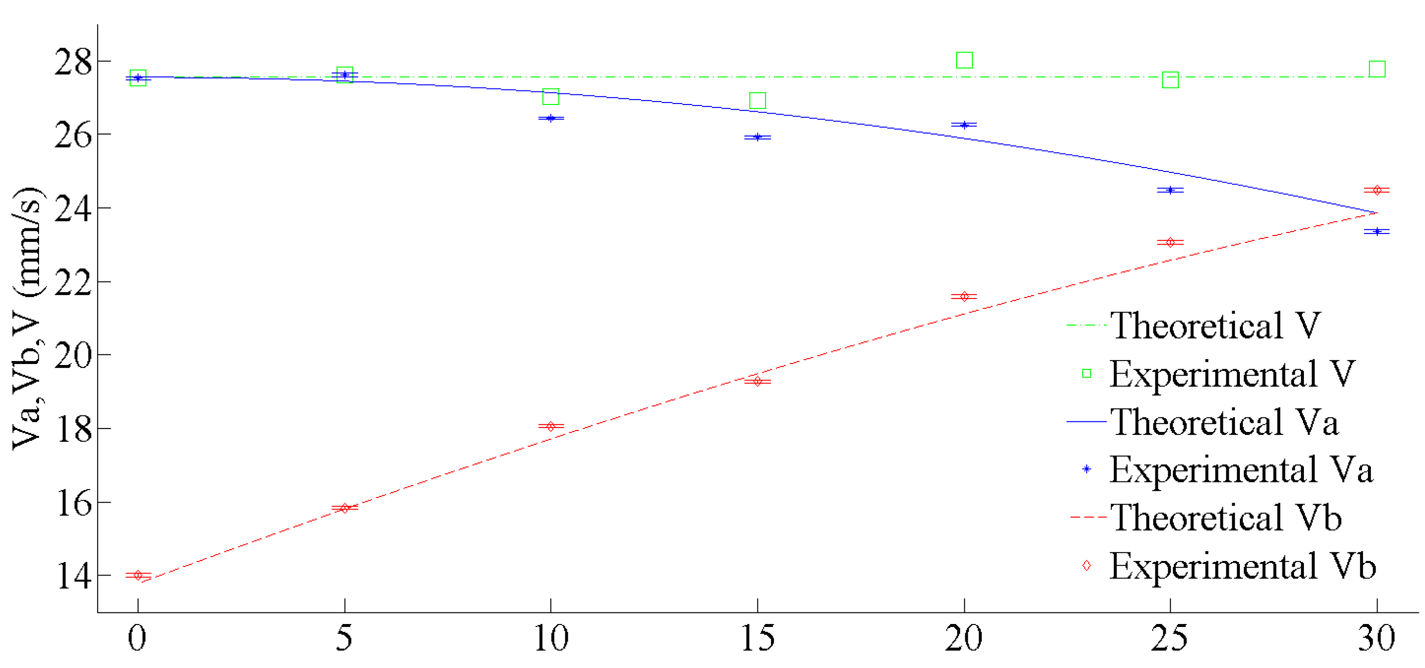
α (°)	Va (mm/s)	Vb (mm/s)	V (mm/s)
0	27.53	14.01	27.53
5	27.62	15.84	27.45
10	26.44	18.06	27.14
15	25.92	19.28	26.93
20	26.26	21.58	28.01
25	24.49	23.07	27.50
30	24.48	24.48	27.78

. Based on the data in Table 1, Figure 7 illustrates the trend of the particle velocities with different direction angles. Note that the theoretical speed component is calculated by giving different angles to Equations (1) and (2). It can be seen that as the incident angle of the particle increases from 0 to 30°, the measured velocity V_a decreases, but at same time, the measured velocity V_b increases. There is only a small fluctuation of the measured velocity V. Observing the relationship between the measured velocity and the theoretical velocity, it is found that the change of the measured velocity is the same as the trend of the theoretical velocity, that is, the theoretical velocity V_a decreases and the measured velocity V_a also decreases. The theoretical velocity V_b increases, and the measured velocity V_b also increases. The theoretical velocity V remains unchanged, and the measured velocity V fluctuates only slightly. To sum up, the measured 2D movement velocity of the particles is consistent with the theoretical trend. The above data can reflect the change of the speed value caused by the change of the movement angle, so the sensor has the ability to measure particle velocity in two dimensions. Error bars for V_a and V_b at different particle angles are also shown in Figure 7. Error bars are calculated by standard deviation and based on three repeated measurements of each velocity component.

Measured V_a and V_b with error bars at different actual velocities of the moving particle are shown in Figure 8a,b. Error bars were calculated by standard deviation and are based on three repeated measurements of each velocity component. According to the measured V_a and V_b, the measured particle velocity V can be calculated by Equations (1) and (2). Figure 8c shows the measured velocity and actual velocity of the moving particle. The measured velocity is consistent with actual velocity within an error of 2%.

In fact, the size of the particle matters because the size of the particle affects whether it is suitable for the sensor. The geometric distribution of seven-core end defines the size of the measurable particles as shown in Figure 9. Considering a spherical particle, theoretically, for the upper limit of particle size, the particle should not completely block the hexagon formed by seven cores as the sensor signal may not contain enough valid details of velocity information, so the diameter of the particle should not be larger than the diagonal length (91 μm) of the hexagon formed by the seven cores. For the lower limit of particle size, the particle should not be too small to pass through the gap among cores without passing through any cores, in order to prevent the sensor from measuring any signal. According to the requirement, the calculated distance of the gap is 28 μm, so the lower limit of particle diameter is 28 μm. Hence theoretically, a spherical particle whose diameters range is from 28 to 91 μm is measurable. Please note that the above estimation is based on the ideal case that the particle is spherical. In reality, non-spherical particles not within the above sizes may also be measured as the projection of non-spherical particles and may meet the requirements.

4. Discussion

Compared with our previous work in which a fiber array probe was used to measure particle velocity in one-dimensional space, the MCF probe in this work not only achieved the velocity measurement in 2D space, but also increased the measurement accuracy. In order to prove that, a brief comparison was conducted between the MCF probe and the fiber array probe by measuring the velocity of a same particle. The fiber array probe was constructed from eight discrete fibers (with 62.5 μm core diameters and 125 μm cladding diameters), which were manually arranged in a plastic plate having a v-groove and fixed with adhesives.

Table 2. Comparison of the particle velocity measurement between the MCF probe and the fiber array probe.

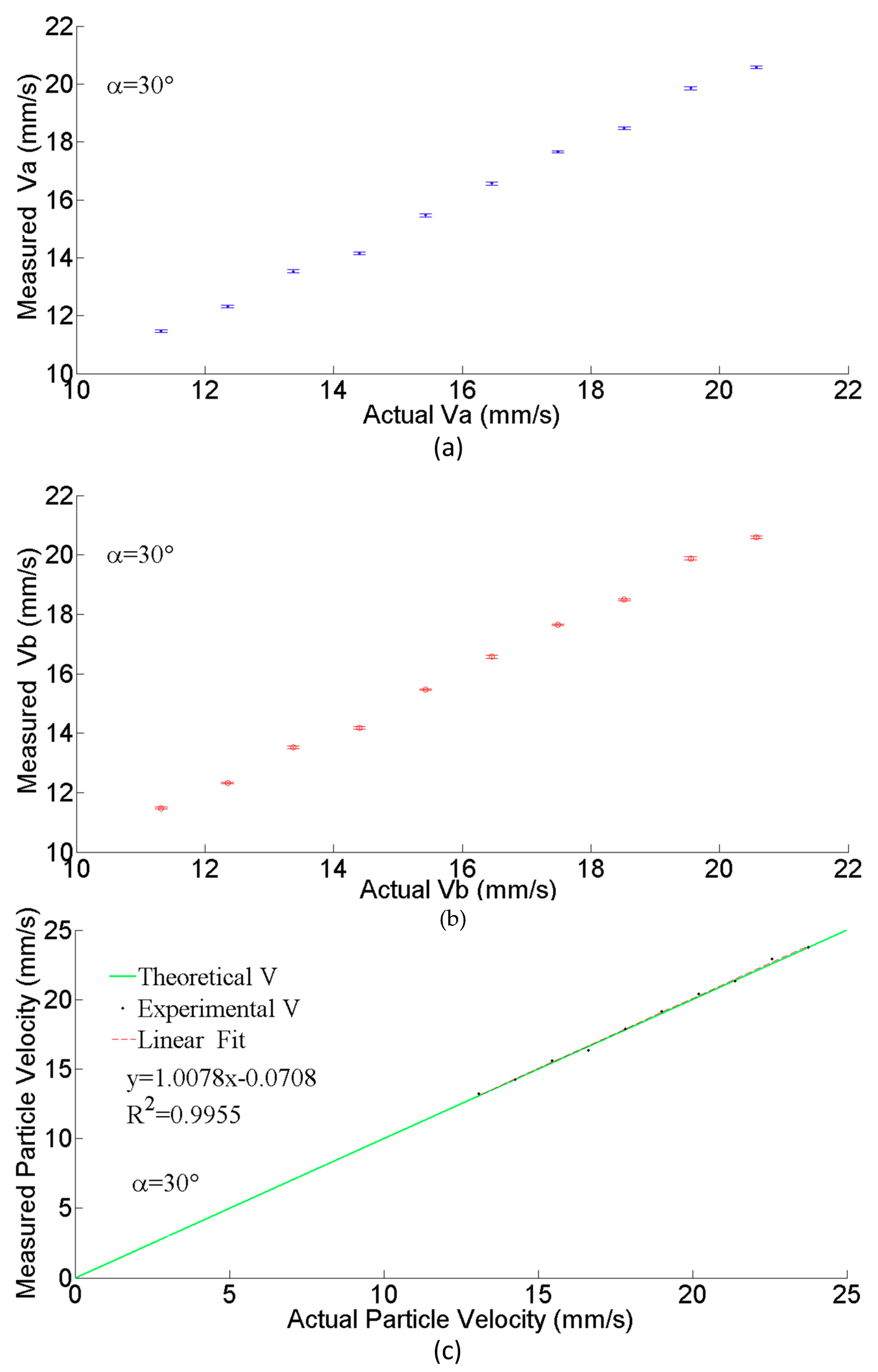
Actual Velocity (mm/s)	Velocity Measured by MCF (mm/s)	Relative Error Measured by MCF (%)	Velocity Measured by Fiber Array (mm/s)	Relative Error Measured by Fiber Array (%)
13.07	13.25	1.38	12.58	3.75
15.44	15.62	1.17	15.27	1.10
17.82	17.84	0.11	17.16	3.70
20.2	20.4	0.99	19.76	2.18
22.57	22.93	1.60	23.09	2.30
23.73	23.75	0.08	24.63	3.79

shows the comparison result of the velocity measurement. We can see that the measurement accuracy of the MCF probe was generally better than that of the fiber array probe. That is because according to the principle of SFV, the interval of the spatial filter p_j affects frequencies of signals received by photo detectors, so the inhomogeneous interval leads to inaccuracy in the determination of the velocity components. For both the MCF probe and fiber array probe, the more consistent the distance (p_j) between cores, the better the measurement will be. As core distances are set during the fiber preform fabrication, they can be checked precisely, so the uniformity of core arrangement is better than the fiber array probe, which is manually assembled. Compared with the method used by Zhou et al. [10], the probe only measures the one-dimensional velocity of the particle, and each optical fiber used to receive the reflected light signal must be connected to a photodetector; that is, three photodetectors must be used for each measurement direction detector. In our method, the probe can measure the two-dimensional velocity of the particle, and only one photodetector is needed for each measurement direction. Compared with the work using a probe composed of thirty-seven ordinary optical fibers to measure the two-dimensional velocity of particles [11], we used only a single MCF instead of thirty-seven ordinary optical fibers as a probe. Moreover, only three PDs were used in our method while seven PDs were used in the study in [11]. The total cost of the sensor is thus much lower.

5. Conclusions

We used an MCF to design a low-cost and compact probe for single microparticle velocity measurement in 2D space. We translated the MCF into spatial filters peaking up spatial frequency components of the moving particle’s shadow image. Velocity and direction of the single particle were successfully obtained. When the particle movement speed was located between 12 mm/s and 24 mm/s, the measurement error was less than 2%. The total cost of the senor is 3000–5000 US dollars. In future work, the sensing system could be further simplified by reducing the number of devices, such as PD, EDFA and splitter.

References

- Shen, Z.; Cao, J.; Arimoto, R.; Han, Z.; Zhang, R.; Han, Y.; Liu, S.; Okuda, T.; Nakao, S.; Tanaka, S. Ionic composition of TSP and PM2.5 during dust storms and air pollution episodes at Xi’an, China. Atmos. Environ. 2009, 43, 2911–2918. [Google Scholar] [CrossRef]
- Dunn, A.K.; Bolay, H.; Moskowitz, M.A.; Boas, D.A. Dynamic imaging of cerebral blood flow using laser speckle. J. Cereb. Blood Flow Metab. 2001, 21, 195–201. [Google Scholar] [CrossRef] [PubMed]
- Ingolf, M.; Wild, W.; Aschemann, H. Real-time measurement of human blood flow with high temporal and spatial resolution. In Proceedings of the SPIE, San Jose, CA, USA, 14 February 2007; p. 644507. [Google Scholar] [CrossRef]
- Fan, L.; Gao, Y.; Hayakawa, A.; Hochgreb, S. Simultaneous, two-camera, 2d gas-phase temperature and velocity measurements by thermographic particle image velocimetry with ZnO tracers. Exp. Fluids 2017, 58, 1–12. [Google Scholar] [CrossRef]
- Gao, Y.; Yang, X.; Fu, C.; Yang, Y.; Li, Z.; Zhang, H.; Qi, F. 10 kHz simultaneous PIV/PLIF study of the diffusion flame response to periodic acoustic forcing. Appl. Opt. 2019, 58, 112–120. [Google Scholar] [CrossRef] [PubMed]
- Ojo, A.O.; Fond, B.; Abram, C.; Van Wachem, B.G.; Heyes, A.L.; Beyrau, F. Thermographic laser Doppler velocimetry using the phase-shifted luminescence of BAM: Eu2+ phosphor particles for thermometry. Opt. Express 2017, 25, 11833–11843. [Google Scholar] [CrossRef] [PubMed]
- Fond, B.; Abram, C.; Heyes, A.L.; Kempf, A.M.; Beyrau, F. Simultaneous temperature, mixture fraction and velocity imaging in turbulent flows using thermographic phosphor tracer particles. Opt. Express 2012, 20, 22118–22133. [Google Scholar] [CrossRef] [PubMed]
- Ushizaka, T.; Asakura, T. Measurements of flow velocity in a microscopic region using a transmission grating. Appl. Opt. 1983, 22, 1870–1874. [Google Scholar] [CrossRef] [PubMed]
- Liu, J.; Grace, J.R.; Bi, X. Novel multifunctional optical-fiber probe: I. Development and validation. AIChE J. 2003, 49, 1405–1420. [Google Scholar] [CrossRef]
- Zhou, J.; Grace, J.R.; Lim, C.J.; Brereton, C.M.H. Particle velocity profiles in a circulating fluidized bed riser of square cross-section. Chem. Eng. Sci. 1995, 50, 237–244. [Google Scholar] [CrossRef]
- Tayebi, D.; Svendsen, H.F.; Grislingas, A.; Mejdell, T.; Johannessen, K. Dynamics of fluidized-bed reactors. Development and application of a new multi-fiber optical probe. Chem. Eng. Sci. 1999, 54, 2113–2122. [Google Scholar] [CrossRef]
- Tani, N.; Kondo, H.; Mori, M.; Hishida, K.; Maeda, M. Development of fiberscope PIV system by controlling diode laser illumination. Exp. Fluids 2002, 33, 752–758. [Google Scholar] [CrossRef]
- Ma, X.; Deng, S.; Li, X. Microparticle velocity sensing using a conical lens fiber array. Appl. Opt. 2019, 58, 3742–3747. [Google Scholar] [CrossRef]
- Abe, Y.; Shikama, K.; Ono, H.; Yanagi, S.; Takahashi, T. Fan-in/fan-out device employing v-groove substrate for multicore fibre. Electron. Lett. 2015, 51, 1347–1348. [Google Scholar] [CrossRef]
- Li, F.; Zhong, H.; Wang, Y.; Kang, Y.; Huang, D.; Guo, Y. Performance Analysis of Continuous-Variable Quantum Key Distribution with Multi-Core Fiber. Appl. Sci. 2018, 8, 1951. [Google Scholar] [CrossRef]
- Wang, W.; Qiu, S.; Xu, H.; Lin, T.; Meng, F.; Han, Y.; Qi, Y.; Wang, C.; Hou, L. Trench-Assisted Multicore Fiber with Single Supermode Transmission and Nearly Zero Flattened Dispersion. Appl. Sci. 2018, 8, 2483. [Google Scholar] [CrossRef]
- YOFC Company. Multi Core Fiber (MCF). Available online: https://en.yofc.com/index.php/view/2349.html (accessed on 30 November 2018).