Vertical Correlation and Array Gain Analysis for Vertical Line Array in Deep Water

Abstract

Array gain (AG) is significant in evaluating the detection performance of the vertical line array, which is directly determined by the correlation of signal and noise, respectively. In this paper, we analyze the vertical correlation for a 16-element vertical line array experimented in the deep ocean in 2016. The ray interference theory is utilized to interpret the mechanism of the vertical correlation of the sound field in different zones. In the direct-arrival zone, the direct rays and once-surface-reflected rays are two dominated components, whose arrival time difference for each element are nearly the same, and the vertical correlation is high. In the shadow zone, the sound field is mainly dominated by bottom-reflected rays and the vertical correlation decreases due to different grazing angles and arrival times of each ray. Different from the previous assumption of noise independence, the effect of noise correlation on the AG is analyzed through the measured marine environmental noise. Results indicate that the noise correlation coefficients in two zones are low but not 0. In the direct-arrival zone, AG is about 10 dB, very close to the ideal value of $10\log M$. AG even exceeds it when NG is negative. Moreover, AG in the direct-arrival zone is higher than the one in the shadow zone.

1. Introduction

Array gain (AG) is a crucial factor for the detection sensor system, which describes the improvement of the signal-to-noise ratio (SNR) between the sensor array and the single element. It can also be expressed as the difference between the signal gain (SG) and the noise gain (NG), which are related to the spatial correlation of the signal and noise, respectively [1]. Spatial correlation of sound field characterizes the similarity of the received signal at different spatial locations. Because of the high correlation of signal received for the horizontal line array, the AG is easy to obtain by using the beamforming technology. However, for the vertical line array (VLA), the received signals of each element contain a complex multipath structure and the signal correlation at different depths is usually not high enough. Thus, and it leads to rapid performance degradation in the beamforming processing.

Previous researches of the vertical correlation in the acoustic field are focused on the shallow water environment. Wan et al. pointed out that when the source and the sensor array are below the thermocline, the vertical correlation length as a function of element interval in units of wavelength increases with frequency and range [2]. In the multipath channel, a method has been proposed to estimate the vertical correlation of the sound field averaged over depths and ranges. Correlation peak appears at the same reception depth as the source depth while ignoring the surface loss and volume absorption [3]. An experiment was conducted in the shadow water, and conclusion reveals that vertical correlation depends on the horizontal range rather than element depth when the received signal at low frequency is in the iso-velocity shallow water with a silt-sand bottom [4]. Vdovicheva et al. compared influence of different carrier frequencies on correlation characteristics when considering irregular acoustic channel boundary. The result indicates that the vertical correlation decreases as the central frequency increases [5].

In comparison with the shallow water, the multipath effect for the long-range sound waves is distinctly weaker in the deep water. Ray theory is applied to estimate the vertical correlation in the multipath channel [6]. Reference [7] infers that the vertical correlation in the deep water is closely related to the hydrophone spacing, signal frequency, and signal waveform distortion caused by multipath interference in the sound field. Then, the coupled-mode theory is applied to analyze the influence of the signal frequency and receiving range on the vertical correlation [8]. Li et al. conducted a deep-water experiment in the South China Sea, and they discussed the vertical correlation of the acoustic field in large depths. Results reveal that in the convergence zone, vertical correlation coefficient periodically oscillates as the receiving depth increases [9].

Noise correlation is another vital factor that makes a great influence on the AG. Cron and Sherman proposed the typical isotropic noise model and the surface noise model and discussed their spatial correlation [10]. Following consideration of the seawater attenuation, the spatial correlation of the wind-driven noise in deep water is analyzed [11,12]. In addition to the classical noise models above, scholars have explored the spatial correlation of multiple noise models. Yang et al. modelled the low-frequency marine environmental noise field in the direct-arrival zone. They discussed the vertical directivity and spatial correlation under three wind speeds by using the ray method and parabolic equation [13]. The characteristic of shipping noise is studied, and spatial correlation functions are also derived from the directionality density function [14].

Based on the development of the correlation theory for the acoustic field, AG research of the VLA is also carried out. Under the Gaussian White noise assumption in deep water, AG of the VLA in the range-independent and weak range-dependent waveguide disturbed by the random internal waves are estimated [15]. Moreover, the modelling method for the ambient noise field caused by the wind is proposed, the AG of the VLA in the non-isotropic noise field affected by wind-driven ambient noise is analyzed [16]. Some researches take SG and NG into account separately and discuss their impact on AG. With a lossy boundary, Buckingham found that the SG is expressed as a superposition of normal modes and the NG is represented as a linear sum of plane waves. In this case, AG of a broadside VLA deployed in shallow sea channel was analyzed [17]. Qiu et al. discussed the spatial gain of the VLA laid in the reliable acoustic path and the direct-arrival zone, respectively. It also demonstrates that when the signal is in the reliable acoustic path, higher array gain can be obtained [18]. In this paper, based an experiment in the Deep South China Sea, the vertical correlation of the sound field in the direct-arrival zone and shadow zone are analyzed, and the correlation coefficient of the noise field is calculated. From the view of ray interference theory, we discuss the sound rays type and arrival structure to explain the mechanism of the vertical correlation of sound field. Finally, the SG and NG and AG are evaluated based on the correlation coefficients of the signal and noise, respectively.

This paper is organized as follows. In Section 2, we introduce the fundamental theory. A simulation calculation is conducted to analyze the effects of correlation coefficient on spatial AG in Section 3. Section 4 discusses the sea trial results. Section 5 summarizes the conclusions.

2. Basic Theory

2.1. Conventional Beamforming Technology

Supposing that there is a vertical line array composed of M elements and the sound source is deployed in the far-field, the output of the gth element is expressed as follows according to the plane wave theory.

$$x_g\left(t\right)=s_g\left(t-\tau \right)+n_g\left(t\right)\mathrm{g}=1,2,\cdots M$$

(1)

where $s_g\left(t-\tau \right)$ and $n_g\left(t\right)$ are received signal and noise of gth hydrophone, respectively, $\tau =\left(g-1\right)d\cos \theta /c$ denotes the signal time delay between the reference element and gth element, $\theta$ is the elevation angle of the incident sound wave, $d$ is the element interval for the line array, and $c$ denotes the sound speed.

Equivalently, in the frequency domain, the form of Equation (1) can be written as

$$X_g\left(f\right)=S_g\left(f\right)e^{-i2\pi f\left(g-1\right)d\cos \theta /c}+N_g\left(f\right)\mathrm{g}=1,2,\cdots M$$

(2)

where $S_g\left(f\right)$ and $N_g\left(f\right)$ are signal and noise spectrum at frequency $f$, respectively.

The received signal and noise of the whole line array can be expressed as

$$X\left(f\right)=A\left(\theta \right)S\left(f\right)+{\rm N}\left(f\right)$$

(3)

where $A\left(\theta \right)$ is a vector of the array manifold, $S\left(f\right)$, $N\left(f\right)$, and $X\left(f\right)$ represent the received signal matrix, received noise matrix, and array output signal matrix, respectively. After passing through the delay-sum narrowband beamformer, the beam output of the line array in forms of the matrix is given by

$$Y\left(f\right)={\mathit{w}}^H\mathit{X}\left(f\right)$$

(4)

where $\mathit{w}$ is the weight vector that can be denoted as

$$\mathit{w}={\left[1e^{i2\pi fd\cos \theta /c}\cdots e^{i2\pi f\left(g-1\right)d\cos \theta /c}\right]}^T\mathrm{g}=1,2,\cdots M$$

(5)

Further, the power output can be expressed as

$$P\left(\theta \right)={\left|\mathit{Y}\left(f\right)\right|}^2={\mathit{w}}^H{\mathit{R}}_{xx}\mathit{w}={\mathit{w}}^H{\mathit{R}}_s\mathit{w}+{\mathit{w}}^H{\mathit{R}}_n\mathit{w}$$

(6)

where ${\mathit{R}}_{xx}=E\left\{\mathit{X}\left(f\right){\mathit{X}}^H\left(f\right)\right\}$ is the covariance matrix of the array, $R_s$ and $R_n$ are the signal covariance matrix and noise covariance matrix, respectively.

In Equation (6), when the power output $P\left(\theta \right)$ reaches its maximum value, $\theta$ corresponds to the estimated elevation angle of the incident sound wave.

2.2. Vertical Correlation Coefficient

The vertical correlation coefficient describes the similarity of the signal received at the same horizontal range but different depths. It is a critical factor which greatly affected the AG [19]. The vertical correlation coefficient in the time domain can be expressed as

$$\rho \left(z,z+\Delta z\right)=\frac{{\displaystyle {\int }_{-\infty }^{\infty }{p}_z\left(t\right)p_{z+\Delta z}\left(t+\tau \right)dt}}{\sqrt{{\displaystyle {\int }_{-\infty }^{\infty }{\left|p_z\left(t\right)\right|}^{2}dt\cdot {\displaystyle {\int }_{-\infty }^{\infty }{\left|p_{z+\Delta z}\left(t\right)\right|}^{2}dt}}}}$$

(7)

where $p_z\left(t\right)$, $p_{z+\Delta z}\left(t\right)$ is the time-domain signal received by two hydrophones in the vertical direction, respectively. $\Delta z$ denotes the vertical spacing of two sensors. In general, in the deep water environment, the signal does not reach each element of VLA at the same time. Thus, the signals are necessary to be compensated before correlation processing.

The vertical correlation coefficient in the frequency domain can be written as

$$\rho \left(z,z+\Delta z\right)=\frac{\mathrm{Re}\left[{\displaystyle {\int }_{{\omega }_1}^{{\omega }_2}{p}_z\left(\omega \right)p_{z+\Delta z}\ast \left(\omega \right)e^{\text{-}i\omega \left(g-1\right)d\cos \theta /c}d\omega }\right]}{\sqrt{{\displaystyle {\int }_{{\omega }_1}^{{\omega }_2}{\left|p_z\left(\omega \right)\right|}^{2}d\omega \cdot {\displaystyle {\int }_{{\omega }_1}^{{\omega }_2}{\left|p_{z+\Delta z}\left(\omega \right)\right|}^{2}d\omega }}}}$$

(8)

where the superscript symbol $\ast$ stands for the conjugation operation, $\mathrm{Re}[\cdot ]$ represents the real part of the content in brackets, $p_z\left(\omega \right)$ and $p_{z+\Delta z}\left(\omega \right)$ are spectrums of the signal received at two different hydrophone depths, respectively. ${\omega }_1$ and ${\omega }_2$ are the angular frequencies, which are determined by the filtering frequency band of the signal. Generally, Equation (7) is usually used to calculate correlation in the experimental data analysis while Equation (8) is utilized for theoretical calculation.

The correlation of the noise received is another critical factor that directly influences the AG analysis. Generally, the isotropic noise and surface noise are two typical and widely used noise models. The isotropic noise field is composed of the combination of sound waves radiated from noise sources uniformly distributed over the sphere, and its vertical correlation coefficient can be expressed by [10]

$${\rho }_{mn}=\frac{\sin \left(2\pi D/\lambda \right)}{2\pi D/\lambda }m,n=1,2,\cdots M$$

(9)

where $D$ denotes the distance between two receivers and $\lambda$ stands for the wavelength of signal.

The surface noise field is made up of sound waves radiated from noise sources distributed on an infinite surface with the ${\cos }^l\left(\theta \right)$ radiation directivity pattern.

Generally, when $l=1$ the correlation coefficient of noise received between two receivers can be shown as [10]

$${\rho }_{mn}=2\frac{J_1\left(2\pi D/\lambda \right)}{2\pi D/\lambda }m,n=1,2,\cdots M$$

(10)

where $J_1$ is 1$th$ Bessel function. These two noise models are usually used for theoretical analysis and comparison with real marine environmental noise.

2.3. Signal Gain and Noise Gain

As mentioned above, array gain is defined as the improvement of the signal-to-noise ratio (SNR) between the hydrophone array and the single element, which can be written as

$$AG=10\log \frac{{\left(S/N\right)}_{array}}{{\left(S/N\right)}_{element}}=10\log \frac{{\left|{\displaystyle \sum _{g=1}^M{s}_g{}^{\prime }\left(f\right)}\right|}^2/{\left|{\displaystyle \sum _{g=1}^M{n}_g{}^{\prime }\left(f\right)}\right|}^2}{{\sigma }_s{}^2/{\sigma }_n{}^2}$$

(11)

where $s_g{}^{\prime }\left(f\right)$ and $n_g{}^{\prime }\left(f\right)$ are spectrums of signal and noise of gth hydrophone after time-delay compensation, respectively, ${\sigma }_s{}^2$ and ${\sigma }_n{}^2$ are signal power and noise power of the single element. After expanding the square term of absolute value in Equation (11), the expression can be deduced as

$$AG=10\log \left[\frac{\left({\sigma }_s{}^2/{\sigma }_n{}^2\right)\cdot {\displaystyle \sum _{u=1}^M{\displaystyle \sum _{v=1}^M{\left({\rho }_s\right)}_{uv}/}}{\displaystyle \sum _{u=1}^M{\displaystyle \sum _{v=1}^M{\left({\rho }_n\right)}_{uv}}}}{{\sigma }_s{}^2/{\sigma }_n{}^2}\right]$$

(12)

Taking the further simplification of Equation (12), the AG is only decided by the correlation coefficients of signal and noise, which can be calculated by

$$AG=10\log \left[\frac{{\displaystyle \sum _{u=1}^M{\displaystyle \sum _{v=1}^M{\left({\rho }_s\right)}_{uv}}}}{{\displaystyle \sum _{u=1}^M{\displaystyle \sum _{v=1}^M{\left({\rho }_n\right)}_{uv}}}}\right]$$

(13)

The expression of AG in Equation (13) can be divided into two parts, the numerator and the denominator, into which a common factor is introduced. The new numerator and denominator are redefined as the signal gain and noise gain, which takes the following form

$$SG=10\log \left[\frac{{\displaystyle \sum _{u=1}^M{\displaystyle \sum _{v=1}^M{\left({\rho }_s\right)}_{uv}}}}{{\displaystyle \sum _{u=1}^M{\displaystyle \sum _{v=1}^M{\left({\rho }_{is-n}\right)}_{uv}}}}\right]$$

(14)

$$NG=10\log \left[\frac{{\displaystyle \sum _{u=1}^M{\displaystyle \sum _{v=1}^M{\left({\rho }_n\right)}_{uv}}}}{{\displaystyle \sum _{u=1}^M{\displaystyle \sum _{v=1}^M{\left({\rho }_{is-n}\right)}_{uv}}}}\right]$$

(15)

where ${\rho }_{is-n}$ denotes the correlation coefficient of isotropic noise, whose formula is shown in Equation (9). The array gain is redefined as the difference between the signal gain and noise gain, and thus it can be written in the form of dB as

$$AG=SG-NG$$

(16)

When the noise is isotropic, and the element interval is equal to half wavelength, the cross-correlation terms of the noise correlation matrix degenerate to zeroes. When the sound source radiating a single plane wave is placed in the far-field, the received signals of two arbitrary hydrophones are entirely correlated. Therefore, the numerator of Equations (14) and (15) can be reduced to

$${\displaystyle \sum _{u=1}^M{\displaystyle \sum _{v=1}^M{\left({\rho }_s\right)}_{uv}}}=M^2$$

(17)

$${\displaystyle \sum _{u=1}^M{\displaystyle \sum _{v=1}^M{\left({\rho }_n\right)}_{uv}}}=M$$

(18)

Further, the signal gain and noise gain take the simplified form as

$$SG=10\log \frac{M^2}{M}=10\log M$$

(19)

$$NG=10\log \frac{M}{M}=0$$

(20)

Under these assumptions, AG of the VLA can reach its ideal value of $10\log M$ in the isotropic noise field through conventional beamforming technology. It should be noted that NG is probably negative because of weak correlation, and thus AG can exceed the ideal value. This situation significantly improves array performance.

3. Simulation Calculation

The isotropic assumption of the ambient noise is usually not satisfied in the ocean environment. Furthermore, the surface noise model is more widely used. According to the Equations (9) and (10), Figure 1 shows the correlation coefficient curves of the isotropic noise and the surface noise with the change of element interval-to-wavelength ratio $d/\lambda$, respectively. Curves indicate that the first zero points of the correlation coefficient curve for the isotropic noise appears at the location of $d=0.5\lambda$ and for the surface noise appears at the location of $d=0.37\lambda$. The noise correlation coefficient in the isotropic noise field is 0.31 When $d=0.37\lambda$ is satisfied. Moreover, correlation coefficients of noise oscillate with the variation of $d/\lambda$.

Section 2 derives the relationship between the array gain and correlation in theory. Next, we conduct a simulation to intuitively validate the effect of variation with signal correlation and noise correlation on the array gain.

In this event, the VLA is deployed in the isotropic noise field, and the element number ranges from 1 to 100. The element interval-to-wavelength ratio is set to be 0.37, 0.5, and 0.7, corresponding to the noise correlation coefficient of 0.31, 0, and −0.22 between adjacent hydrophones, respectively. The correlation coefficient of the signal between adjacent elements is set to be 0.8 and 1, respectively. In the isotropic noise field, the array gains with different noise correlation coefficients and different signal correlation coefficients are calculated and shown in Figure 2. It can be seen that AG decreases as the ${\rho }_s$ decreases, and AG no longer increases when the number of elements increases to a certain quantity. When the ${\rho }_s$ keeps at a fixed value, AG ascends with ${\rho }_n$ descending. When the ambient noise is isotropic, and the signal is completely correlated, AG is equal to $10\log M$, as presented in the purple solid line. In some cases, AG even exceeds the normal value of $10\log M$ as the correlation coefficient of noise between adjacent elements is less than zero.

4. Experimental Results

4.1. Experiment Introduction

The experiment was an acoustic field trial conducted in the South China Sea in 2016, as shown in Figure 3a. The vertical hydrophone line array was composed of 16 elements with an interval of 5 m. The top element was deployed at a depth of 370 m, and the bottom element was about 445 m. The sound source loaded on the ship was at point A and B, where the horizontal range was 2.4 km and 10.3 km, respectively, and the source depth was 30 m. The depth of the whole measurement area was about 1800 m. There were 5 TD sensors (RBRduet T.D) used to record the element depths of the vertical line array. The top hydrophone element was equipped with an electronic compass to record the underwater attitude of the vertical line array. The change of array tilt angle during the experiment is shown in Figure 3b. The narrow-band sound source radiated a single-frequency signal at 350 Hz. The duration of one pulse signal was 5 s, and the interval between the two adjacent pulses was 1 s. The measurement time for each point was half an hour. Considering the time (one hour) for the boat from point A to the point B, the total time for the whole experiment was two hours. The sampling rate was 16 kHz. The sea condition was level 3 and there were no other ships around the experiment site.

The sound velocity profiler (AML-Minos X SVP) was used to measure the sound speed profile (SSP) at both points, and the difference was very small. It can be considered that the variation of the SSP can be ignored in a short time. Therefore, we used the SSP shown in Figure 4a to analyze the sound field. The depth of the deep sound channel is 1041 m with the minimum sound velocity of 1482 m/s. The sound speed near the seafloor is 1491 m/s while that near the surface is 1546 m/s. This is a typical non-full deep water sound channel, where the sound rays reflected by the bottom have a profound influence on the sound field in the shadow zone. The seabed-state parameters obtained after consulting the information are shown at the bottom of Figure 4a.

According to the experiment configuration and measured SSP, the transmission loss is calculated and presented in Figure 4b by using the BELLHOP model. It is indicated that the VLA with a length of 75 m is in the direct-arrival zone when the horizontal range is 2.4 km and in the shadow zone when the range is 10.3 km.

4.2. Correlation and Array Gain in the Direct-Arrival Zone

We collect the acoustic signal data received by the vertical hydrophone line array when the sound source is placed at a depth of 30 m and the horizontal range of 2.4 km. A segment of signal for 30 s is intercepted from the early of the received signal and filtered by a band-pass filter with a frequency range of 300–400 Hz. Therefore, the SNR near the signal frequency is increased. The top element is regarded as the reference element in the following discussion. 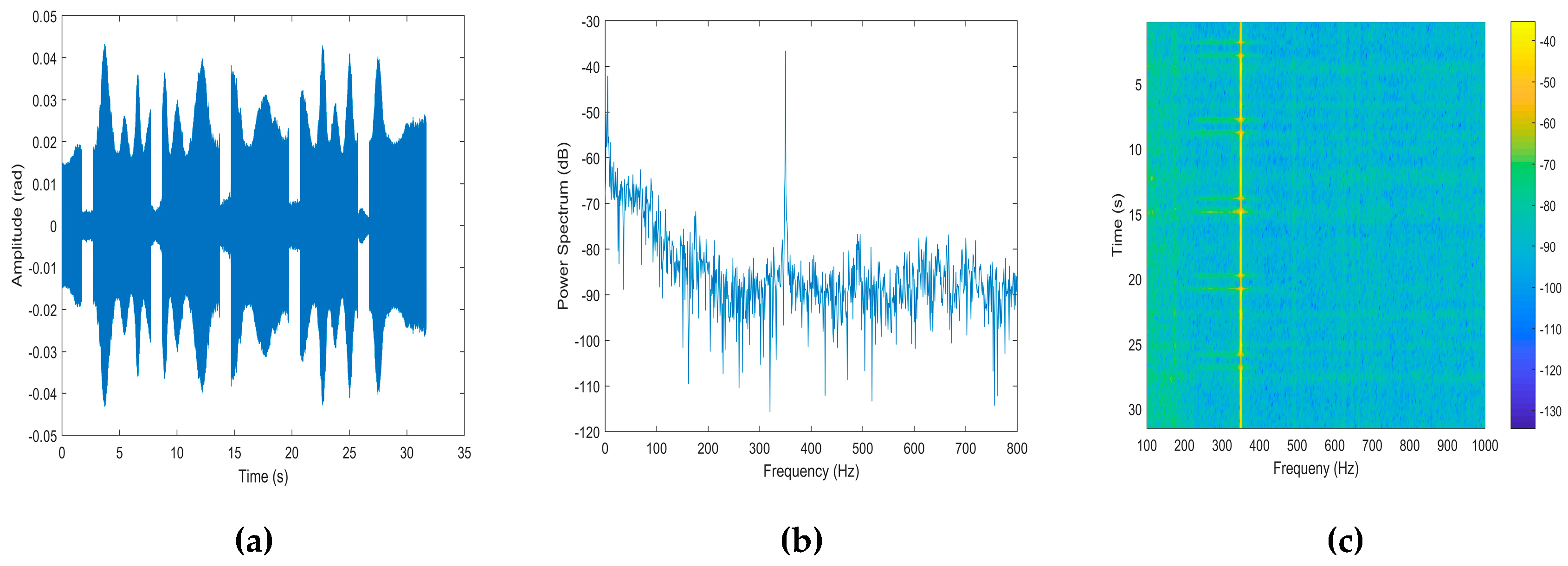Figure 5 shows waveforms of the signal received by the reference element in the time domain, frequency domain, and time-frequency domain. In Figure 5a, because of the high SNR it is obvious to view the pulse shape of the received signal and the reception gap between the two 5-second signals. Figure 5b,c display the signal frequency steadily.

In order to estimate the elevation angle of the sound source, conventional beamforming technology is applied to process the receiving data above. After the time compensation processing, the power output of each beam is shown in Figure 6. The 0° of the elevation angle corresponds to the direction along the vertical array axis and toward the sea surface.

As seen in Figure 6, there are two distinct bright columns at 78° and 133°, respectively. According to the experiment setup, the direction of the received direct-arrival wave is downward. Hence, the real elevation angle of the acoustic source is 78°, and the other power peak of 133° is corresponding to the grating lobe due to $d/\lambda >0.5$. The explanation for the grating lobe is validated through the simulation in Figure 7, in which the element number of the line array is 16, and the element interval is 5 m. The simulation frequency is 350 Hz, and the elevation angle of the sound source is set to 78°. It is indicated that the grating lobe appears at the elevation angle of 133°, which is consistent with the experimental result.

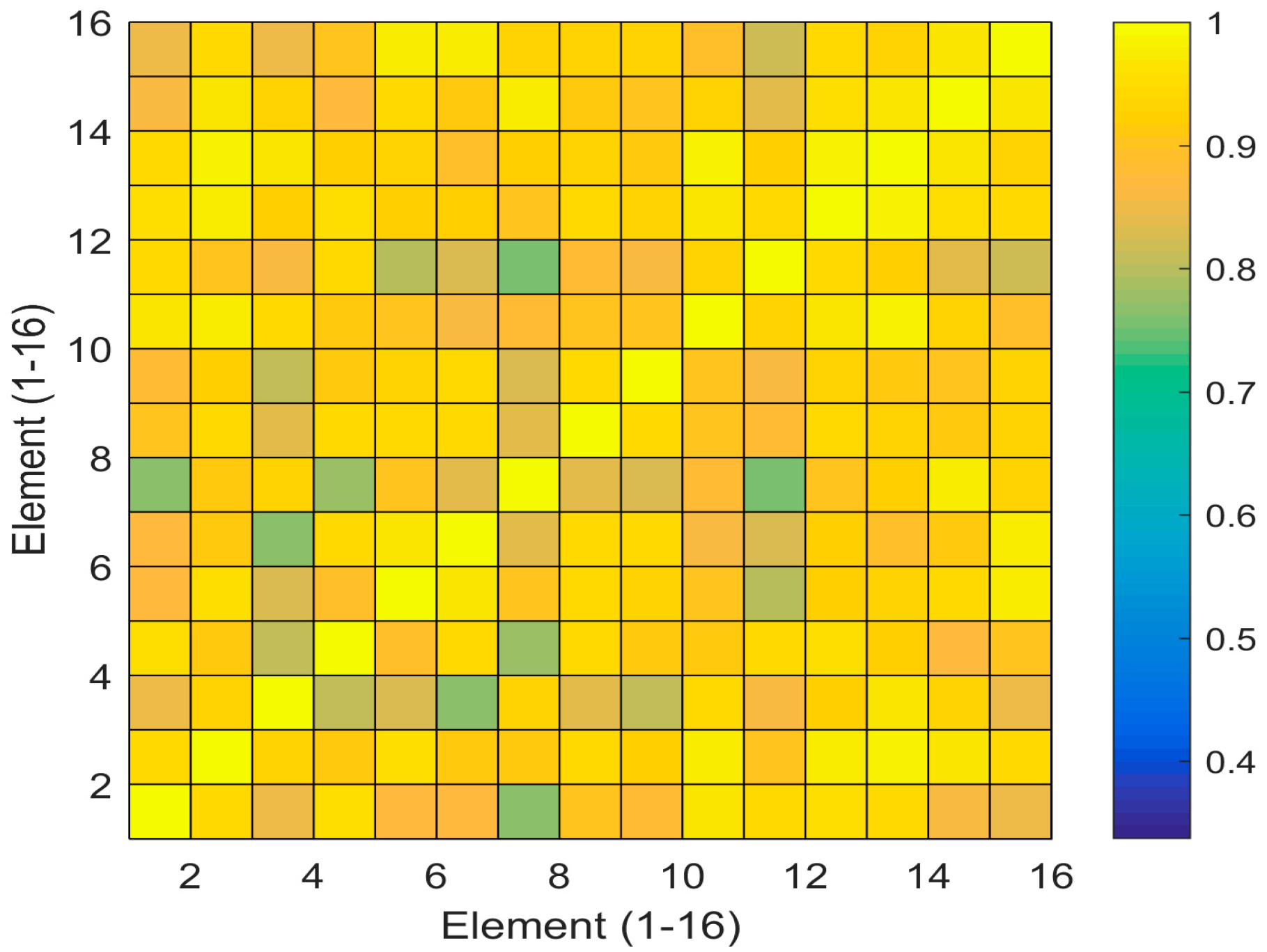
As shown in Section 2, the correlation coefficient of the received signal describes its similarity. Generally speaking, in an unbounded homogeneous medium, the signal from the sound source propagates freely without distortion, and hence, the signal between arbitrary receiving points are completely correlated. However, in the real marine environment, multipath propagation and sound scattering cause the waveform distortion, which results in a decrease of signal correlation. The correlation coefficients of the signal received by the array are calculated and presented in Figure 8. Each square stands for the signal correlation between the element and the reference element. We can see that the value of correlation coefficients slightly descend with the increase of element spacing, but the majority are still higher than 0.7. Also, the correlation coefficients between adjacent elements are nearly equal to 1.

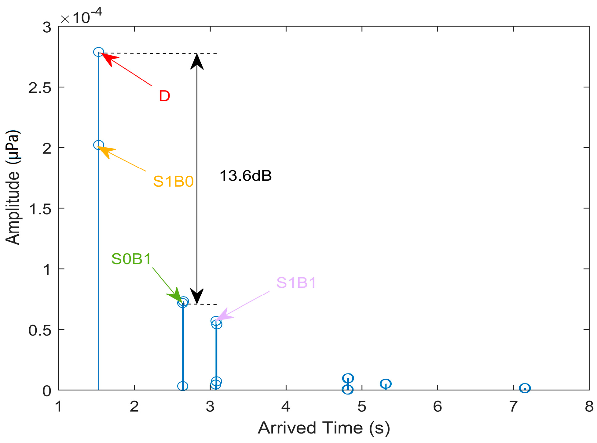
The ray acoustics can better reflect the propagation characteristics of sound waves in the deep sea. In the direct-arrival zone, the high vertical correlation of the acoustic field could be explained by BELLHOP model, which can calculate the time arrival structure, ray trace, and sound intensity in the marine environment. Since the sound source is near the sea, and the array length is a small amount relative to the horizontal range, the receiving structure of the topmost element is not much different from the bottommost element. Substituting the measured SSP into the BELLHOP model, we calculate the time arrival structure of the eigen-rays received by the reference hydrophone in Figure 9. The source depth and receiving range are the same as the actual sea trial conditions. It is apparent that the direct ray (D) and the once-surface-reflected ray (S1B0) are the main components of the sound field, whose energy is higher than other rays. For example, taking the amplitude of the D wave as the reference standard, we find that the amplitudes of the once-bottom-bounce ray (S0B1), and once-surface-reflected and once-bottom-reflected ray (S1B1) are nearly 13.6 dB lower than D wave as the form of dB. This finding occurs mainly because the sound wave incident to the ocean bottom at larger grazing angles will suffer more severe reflection attenuation. As a consequence, the acoustic field in the direct-arrival zone is dominated by D wave and S1B0 wave.

To further explain the high correlation,

Table 1. Structure of D and S1B0 wave.

Type	Amplitude (μPa)	Arrival Time (s)	Arrival Angle (°)	Number of Surface-Reflection	Number of Bottom-Reflection
D	2.78 × 10−4	1.529	15.28	0	0
S1B0	2.02 × 10−4	1.529	15.95	1	0

lists the arrival time and elevation angle of D wave and S1B0 wave for the reference element. From the table, we can see that the amplitude difference between D wave and S1B0 wave is about 7.6 × 10⁻⁵ μPa, namely 2.78 dB, and the arrival time and arrival angles between these two ray components are nearly equal to each other. This phenomenon is similar to other elements.

Ray trace clearly reflects the propagation path of sound energy so that the sound field distribution can be qualitatively interpreted. According to the calculation results above, the ray trace of D wave and S1B0 wave received by the reference element are presented in Figure 10. The abscissa represents the horizontal range from the sound source to the receiver. We can see that these two waves propagate almost along the same path and have nearly the same receiving amplitude, arrival time, and arrival angle, which makes their coherent superposition.

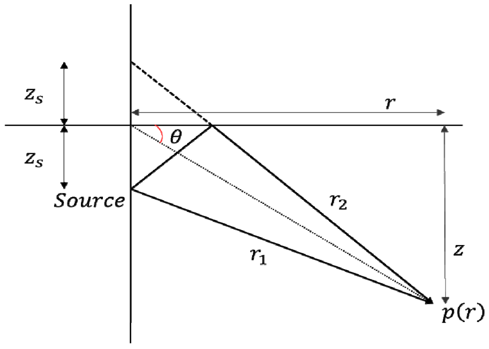
Ray theory can quantitatively analyze the high vertical correlation of sound field. In the direct-arrival zone, we only consider the D wave and S1B0 wave, and other ray components can be ignored. Figure 11 displays the interference schematic diagram of two rays. We assume that the environment is range independent, the sound speed between the source and receiver is a constant, and the sea surface is absolutely soft. Thus, the sound rays travel along a straight line and are perfectly reflected by the sea surface. The signal received is the superposition of D wave and S1B0 wave, which can be written as [20].

$$p_z(\omega )=\frac{1}{r_1}{e}^{i\left(k{r}_1-\omega t_1\right)}-\frac{1}{r_2}{e}^{i\left(k{r}_2-\omega t_2\right)}$$

(21)

where $r_1$ and $r_2$ are propagation ranges of the D wave and S1B0 wave, respectively, $t_1$ and $t_2$ are the corresponding propagation time. According to Figure 11, propagation distance of two sound rays is calculated by

$$r_1=\sqrt{r^2+{\left(z-z_s\right)}^2},r_2=\sqrt{r^2+{\left(z+z_s\right)}^2}$$

(22)

where $r$ represents the horizontal range from sound source to receiver, $z$ and $z_s$ denote the receiver depth and the source depth, respectively. The distance $R$ is defined as the linear distance from coordinate origin to receiving point, which satisfies the equation $R^2=r^2+z^2$. Considering that $R\gg z_s$, Equation (22) can be simplified as

$$r_1\simeq R-z_s\sin \theta \approx R,r_2\simeq R+z_s\sin \theta \approx R$$

(23)

where $\theta$ is the angle between the line of the source to the receiving point and the horizontal line. Based on Equation (23), the propagation ranges of D wave and S1B0 wave are nearly equal to each other. Next, we define the propagation time difference between D wave and S1B0 wave as

$$\Delta t=t_2-t_1$$

(24)

Substituting Equations (23) and (24) into (21), the received signal can be expressed as

$$p_z\left(\omega \right)=\frac{1}{R}{e}^{i\left(kR-\omega t_1\right)}\left(1-e^{\text{-}i\omega \Delta t}\right)$$

(25)

Similarly, the signal received by another sensor in the same range can be written as

$$p_{z+\Delta z}\left(\omega \right)=\frac{1}{R^{\prime }}{e}^{i\left(k{R}^{\prime }-\omega t_1{}^{\prime }\right)}\left(1-e^{\text{-}i\omega \Delta t^{\prime }}\right)$$

(26)

where $R$ and $R^{\prime }$ are numerically equal, and both represent the horizontal range of point A. Substituting Equations (25) and (26) into (8) and combined with $R=R^{\prime }$, the correlation coefficients of signal after simplification are given by

$$\rho \left(r_1,r_2\right)=\frac{\mathrm{Re}\left[{\displaystyle {\int }_{{\omega }_1}^{{\omega }_2}{e}^{i\omega \left(t_1{}^{\prime }-t_1\text{-}\tau \right)}\left(1-e^{\text{-}i\omega \Delta t}\right)\left(1-e^{i\omega \Delta t^{\prime }}\right)d\omega }\right]}{\sqrt{{\displaystyle {\int }_{{\omega }_1}^{{\omega }_2}{\left|1-e^{\text{-}i\omega \Delta t}\right|}^{2}d\omega \cdot {\displaystyle {\int }_{{\omega }_1}^{{\omega }_2}{\left|1-e^{\text{-}i\omega \Delta t^{\prime }}\right|}^{2}d\omega }}}}$$

(27)

Based on the experiment setup, the position of source and receivers are specific, in other words, $R$, $z$, and $z_s$ are specific. The real part of $\exp \left[i\omega \left(t_1{}^{\prime }-t_1-\tau \right)\right]$ is approximately equal to the maximum 1 by adjusting time delay $\tau$. As a consequence, the value of correlation coefficient $\rho$ is only determined by $\Delta t$ and $\Delta t^{\prime }$. When considering the single frequency signal, Equation (27) can be written as

$$\rho \left(r_1,r_2\right)=\frac{\left[1+\cos \left({\omega }_0\left(\Delta t^{\prime }-\Delta t\right)\right)-\cos \left({\omega }_0\Delta t^{\prime }\right)-\cos \left({\omega }_0\Delta t\right)\right]}{2\sqrt{\left(1-\cos \left({\omega }_0\Delta t^{\prime }\right)\right)\left(1-\cos \left({\omega }_0\Delta t\right)\right)}}$$

(28)

After further simplification, the correlation coefficient is

$$\rho \left(r_1,r_2\right)=\cos \left(\frac{{\omega }_0}{2}\left(\Delta t^{\prime }-\Delta t\right)\right)$$

(29)

In the direct-arrival zone, when the source is near the surface, the arrival time of D wave and S1B0 wave at any hydrophones almost have no difference, namely $\Delta t^{\prime }\approx \Delta t$ and a high value of $\rho$ can be obtained. Figure 12 shows the theoretical calculation result and experiment result. It is indicated that the trend of the correlation coefficient with the element depth is similar, but Equation (27) only considers the D wave and S1B0 wave which mainly contribute to the sound field. The real received signal also contains the sound energy of other paths, thus, the two curves show difference. The same interpretation method can be extended to non-isosonic profile.

The noise correlation is another significant factor in the evaluation of AG. Generally speaking, because of the high SNR, it is difficult to separate the signal and noise when receiving data. Furthermore, the ambient noise is not expected to change during a short time. Hence, the data received before the signal transmission is regarded as the noise. We measured the actual marine environmental noise to do the next analysis. Figure 13 shows the noise correlation coefficients corresponding to different element interval-to-wavelength ratio. The blue line, red line, and yellow line in Figure 13 denote the measured ambient noise, the isotropic noise model, and the surface noise model. It is indicated that the noise correlation coefficient in the real ocean is higher than those of the two theoretical noise models, although there exists a similar trend. Also, from Figure 13 we reveal that the correlation coefficient of measured noise is 0.2 at the frequency of 350 Hz as shown in purple round, basically close to that of surface noise. Next, the actual noise correlation coefficient of the array is discussed as follows.

Further, the correlation coefficients of noise are calculated by Equation (7) and shown in Figure 14, where the correlation coefficient of the noise received by two adjacent elements is slightly higher than zero. Moreover, as the receiver depth increases, the noise correlation coefficient decreases. In other words, the noise received at different depths is largely uncorrelated to each other.

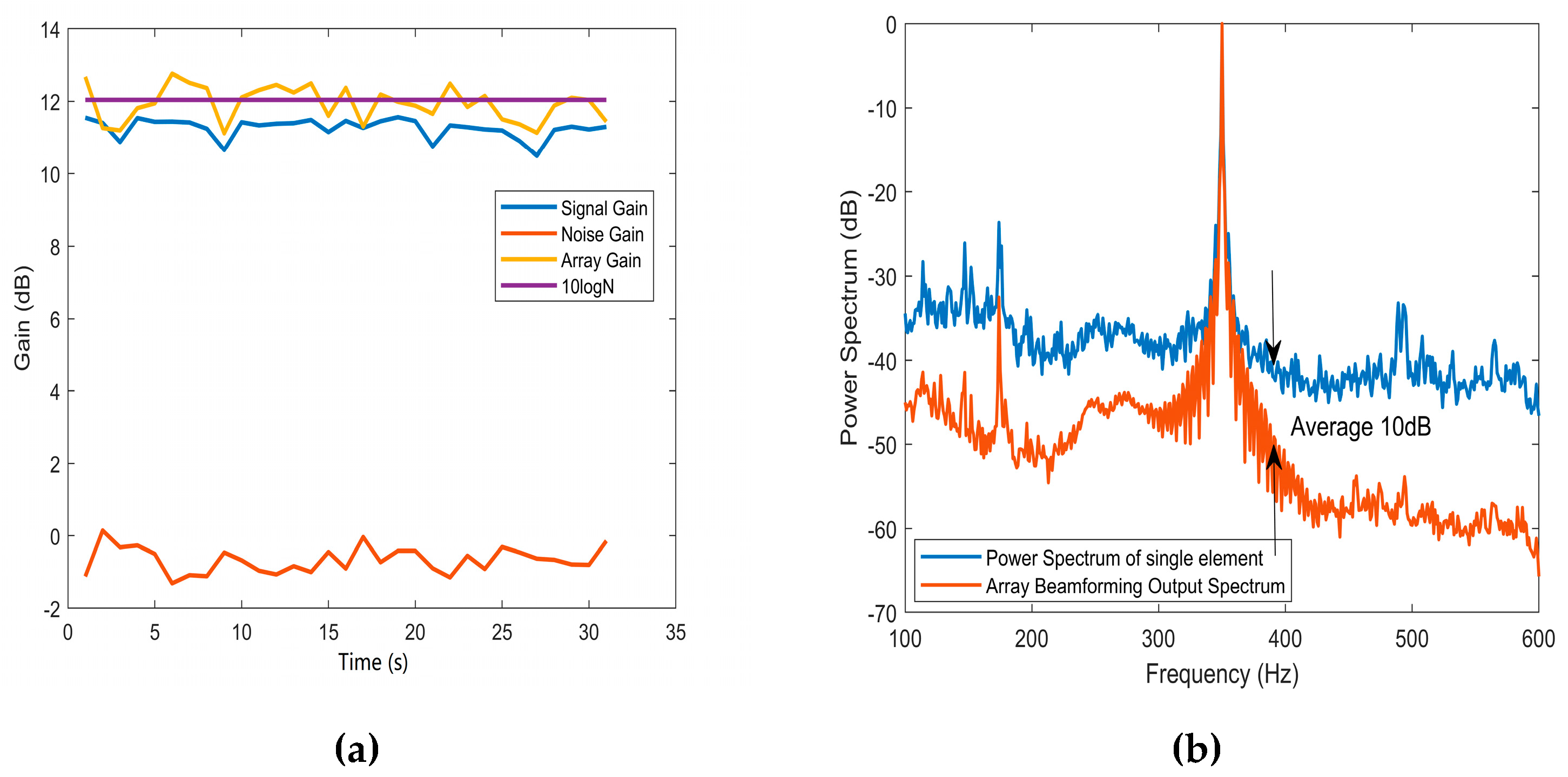
According to the correlation coefficient of signal and noise above, the signal gain, noise gain, and array gain are estimated. In Figure 15a, the blue line, red line, and yellow line represent SG, NG, and AG, respectively. It is manifested that the curve of SG fluctuates around 11 dB and the value of NG ranges from −1 dB to 0 dB. The value of AG fluctuates around the ideal value of 12 dB, and the average value of AG is about 11.9 dB. It is noteworthy that the value of AG exceeds the ideal value of $10\log M$ during the time of 5 s to 8 s. That is because SGs during these periods are very close to $10\log M$, and the corresponding NGs are relatively stable and remain at a negative value.

For validating the AG analysis above, the beamforming output spectrum of the VLA and the power spectrum of a single element are compared and given in Figure 15b. In order to intuitively display the difference between the two spectrums, we normalize the peak corresponding to the signal frequency and thus, the difference of two noise power spectrums among the whole frequency band is regarded as the AG after eliminating outliers. We can see that the average AG is about 10 dB, which is close to the calculation result of 11.9 dB in Figure 15a. In the frequency band from 100 Hz to 200 Hz, there exist some small fluctuated peaks, which are caused by low-frequency environmental noise.

The experimental time for each measurement point is half an hour. To verify the effect of time changes on the array gain, we divide the half-hour measurement time into three segments and intercept 30-s signal from each division to calculate the array gain. Array gains of the early segment (1–10 min) have been discussed in Figure 15b. 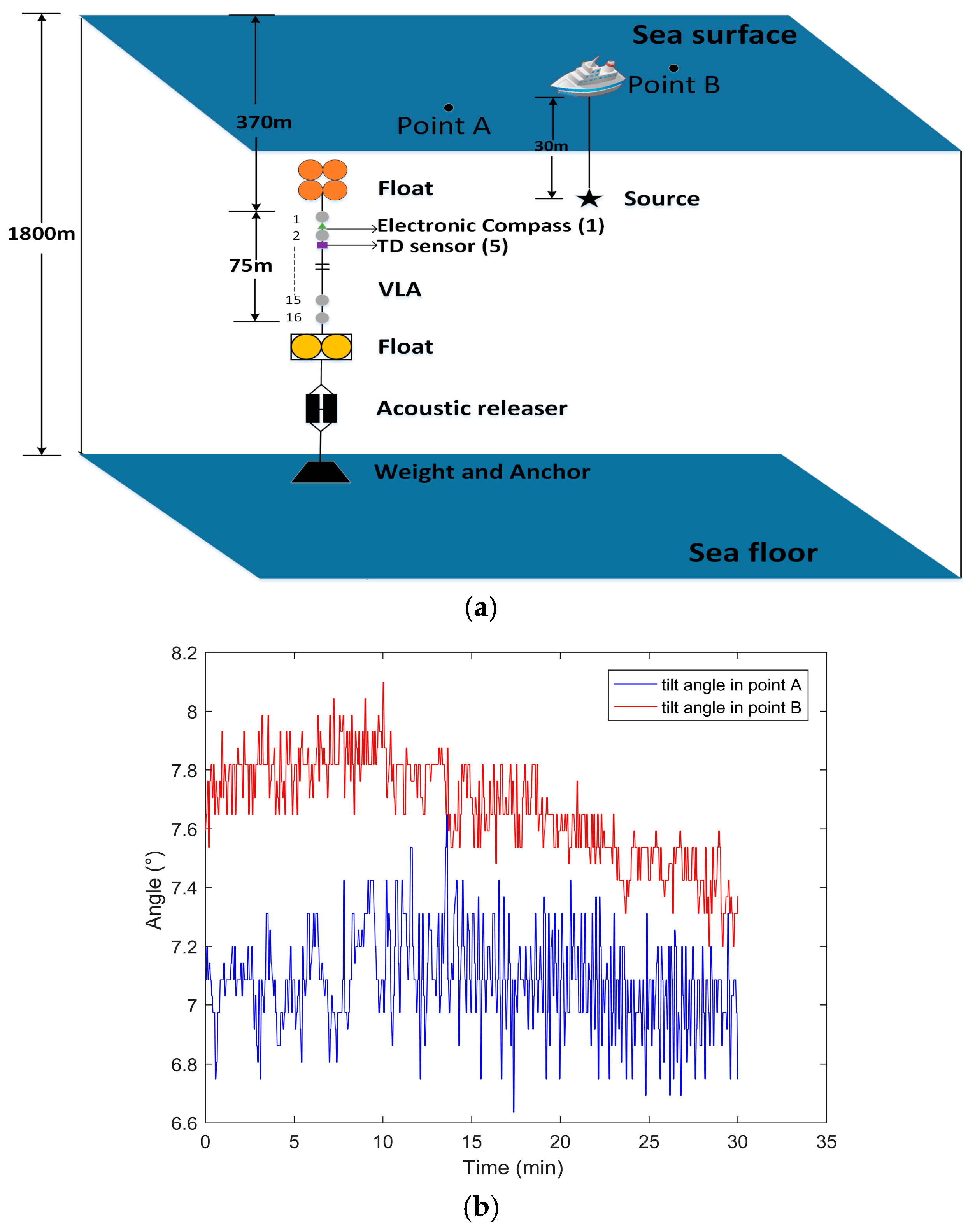Array gains in the middle (11–20 min) and late (21–30 min) period are shown in Figure 16. The average AG in the early, middle, and late period is 10 dB, 9 dB, and 9 dB, respectively. The little difference may be because the marine environment changed slightly during the entire measurement time. Moreover, the tilt angle of the array changed about 1° due to the disturbance of the ocean current (as shown in Figure 3b). It can be concluded that the array gain remains constant basically throughout the measurement time.

In this subsection, we have discussed the correlation and AG in the direct-arrival zone and explained the reason for high value of AG from the perspective of sound rays. Next, the correlation and AG in the shadow zone are analyzed.

4.3. Correlation and Array Gain in the Shadow Zone

When the sound source is placed at a depth of 30 m and a horizontal range of 10.3 km, we collect the signal data received by the VLA. The acoustic field is now located in the shadow zone. 30-s samples of the signal are selected and filtered by a band-pass filter with a frequency range of 300–400 Hz in this processing. The top element is still considered as the reference element. The signal received by the reference element in the time domain, frequency domain, and time-frequency domain is presented in Figure 17, respectively. Because of the significant influence of multiple paths during the propagation of sound waves, pulse shape of the received signal in the time domain is not evident and arrival waves at the various time are mixed, as shown in Figure 17a.

Similarly, the power output of the VLA is shown in Figure 18 after the conventional beamforming processing. From Figure 18, we can find that there exist two visible peaks appearing at 111° and 61°, respectively. According to the experiment configuration, the direction of the received wave is mainly upward in this range. Therefore, the elevation angle of the signal received by hydrophones is 111°, and the grazing lobe angle is 61°.

Following Equation (7), the correlation coefficients of the received signal are calculated and shown in Figure 19. It is concluded that the correlation coefficients between two different hydrophones are lower than those in the direct-arrival zone in Figure 8. Besides, correlation coefficients descend significantly as the vertical depths ascend and show periodic oscillation, as shown in Figure 20. This phenomenon occurs mainly because, at long range, sound rays undergo multiple reflections between the sea surface and the bottom. Moreover, the difference in the arrival time of each ray increases and multi-path interference becomes complicated.

To analyze the ray type in the shadow zone, we use the BELLHOP model to calculate the time arrival structure of the eigen-rays received by the reference hydrophone. As shown in Figure 21a, we can see that the acoustic field in the shadow zone is mainly composed of the once-bottom-bounce ray (S0B1), once-surface-reflected and once-bottom-reflected ray (S1B1), and the twice-surface-reflected and once-bottom-reflected ray (S2B1). It is concluded that the time arrival structure becomes more complicated than that in the direct-arrival zone because of multiple reflections of sound rays from the ocean surface and the ocean bottom. The amplitudes of three types of the ray are close, as presented in Figure 21a. The ray traces of the S0B1 wave, S1B1 wave, and S2B1 wave received by the reference element are further shown in Figure 21b, in which we can find that propagation traces between S1B1 wave with the blue line and S2B1 wave are close. Furthermore, the path of S1B1 wave with purple line and the one of S0B1 wave are also similar. However, there exist different propagation paths and distinct time-delay differences between the two groups, which complicates multi-path interference and reduces the vertical correlation of the sound field.

Table 2. Structure of S1B1, S0B1, and S2B1 wave.

Type	Amplitude (μPa)	Arrival Time (s)	Arrival Angle (°)	Number of Surface-Reflection	Number of Bottom-Reflection
S1B1	9.87 × 10−5	7.218	−10.56	1	1
S0B1	9.17 × 10−5	7.211	−10.56	0	1
S2B1	7.85 × 10−5	7.36	16.59	2	1
S1B1	6.51 × 10−5	7.348	16.59	1	1

shows the amplitudes, arrival time, and elevation angles information of S0B1 wave, S1B1 wave, and S2B1 wave, respectively. In this table, the positive and negative values of the arrival angle represent the downward and upward direction of the incident wave, respectively. Based on the different arrival time, we regard the S1B1 wave with negative angle and S0B1 wave as the first group, and S2B1 wave, S1B1 wave with positive angle as the second group. It is observed from Figure 21a and Table 2 that the first group has a larger amplitude than the second group and the arrival time is earlier. It is because the sound rays of second group incident to the bottom at a large grazing angle and reflection attenuation is severe. Thus, the arrival amplitude decreases accordingly. The second group experiences a longer path, and it arrives later. It is apparent that there is a time difference of nearly 0.15 s between these two groups.

Moreover, the amplitudes of two rays within each group are also different. For example, the amplitude of S1B1 is slightly higher than that of S0B1 because the paths do not entirely coincide. The received signals are a mixture of signal with different arrival angles and powers. In this case, when the signal received is compensated with a single time delay by conventional beamforming technology, signal correlation decreases, accordingly.

Further, we calculate the correlation coefficients of the received noise and show them in Figure 22. The figure shows that noise correlation coefficients are nearly equal to 0 except diagonal elements, which means the received noise is almost uncorrelated for every two different sensors. Compared with the noise received in the direct-arrival zone, the noise correlation in the shadow zone is slightly lower. The reason is that when the array is in the shadow zone, the distance from the sound-source ship to the receivers is significantly further, and there is less ship noise received.

Then, the signal gain, noise gain, and array gain are calculated by the signal and noise correlation coefficients. As shown in Figure 23a, the curve of SG fluctuates around 8 dB because of the weak signal correlation, and the value of NG is about 0 dB. The value of AG is nearly equal to that of SG and is about 4 dB lower than the ideal value of 12 dB. The reason for the lower AG is the time delays of each element cannot be compensated accurately by using only one single angle when the plane wave model is not satisfied. In order to verify the previous discussion, the beamforming output of the VLA and power spectrum of the single element are calculated and shown in Figure 23b. Using the same normalization method as before, the SNR of beamforming output for the VLA is about 7 dB higher than that of the single element, which is very close to the average AG value of 8 dB.

We also intercept three 30-s signals to calculate the array gains. As shown in Figure 24, the average AG in the middle and late segment is 6.5 dB and 5.5 dB, respectively. The marine environment changed with the time slightly, and the tilt angle of the array changed about 1°, which causes a little difference in the AG. We can consider that the AG remains constant basically during the measurement time.

Through the above analysis, it is found that the influence of the measurement time on the array gain can be ignored. Next we discuss the effect of ship auxiliary engine noise on the array gain.

The auxiliary engine of the ship was still working when the ship was stopped in the measurement points. At point A with the horizontal range of 2.4 km, the effect of the auxiliary noise on the marine environment noise cannot be ignored. At point B with 10.3 km, the auxiliary engine noise has a slight effect. We compare the noise correlation between two measurement points, as presented in Figure 25. The noise at point B is basically uncorrelated, and the noise correlation coefficient at point A fluctuates around 0.2. Considering the whole experiment lasting for only two hours, so the changes in the marine environment caused by the time are negligible. The small difference in noise correlation is caused by the auxiliary engine.

According to Figure 15a and Figure 23a, the average noise gain of point A and point B is −0.678 dB and −0.302 dB, respectively, with a difference of only 0.376 dB. Therefore, we can conclude that the auxiliary engine noise has little effect on the array gain and can be ignored.

5. Conclusions

Array gain is a critical factor in evaluating the detection performance for the vertical line array and can be expressed by signal correlation and noise correlation. In this work, based on a trial conducted in the South China Sea, the experimental signal correlation and noise correlation were analyzed when the vertical line array was deployed in the direct-arrival zone and the shadow zone, respectively. Ray interference theory was utilized to analyze the structure of the sound field and interpret the vertical correlation characteristic. Based on the measured marine environmental noise instead of independent noise assumption, the effect of noise correlation on the array gain was analyzed. According to the correlation coefficients, the array gain of the corresponding zone was also discussed. Hence, several conclusions are summarized as follows:

• The correlation coefficient of signal and noise can directly represent signal gain and noise gain, respectively, and the difference between these two gains is the array gain. Positive signal gain and negative noise gain can increase the array gain, which improves the detection ability of underwater targets.
• For the direct-arrival zone, D wave and S1B0 wave are the main components of the sound field, and some waves reflected from the seabed can be ignored. These two waves have almost identical arrival structures and ray traces and add up constructively. Hence, the correlation coefficients of the received signal are close to 1. Accordingly, the measured noise correlation coefficient fluctuates in a small range near 0, and thus the array gain is about 10 dB, nearly equal to the ideal value of 10logM. In some cases, it even exceeds the ideal value.
• For the shadow zone, the sound field is dominated by S1B1 wave, S0B1 wave, and S2B1 wave. There are apparent differences in their arrival time and arrival angle because of the multipath effect. The multipath interference structure of the signal becomes complex. Therefore, the signal correlation coefficient is lower than that in the direct-arrival zone. Its correlation decreases as the vertical depths increase and presents periodic oscillation. Furthermore, the received noise of each element is almost completely uncorrelated. At this time, the value of AG is 7 dB, which is less than the ideal value. The effect of time variation and ship auxiliary noise on the array gain can be neglected during the experiment.

References

1. Hamson, R.M. The theoretical gain limitations of a passive vertical line array in shallow water. J. Acoust. Soc. Am. 1980, 68, 156–164. [Google Scholar] [CrossRef]
2. Wan, L.; Zhou, J.X.; Rogers, P.H.; Knobles, D.P. Spatial coherence measurements from two L-shape arrays in Shallow Water. Acoust. Phys. 2009, 55, 383–392. [Google Scholar] [CrossRef]
3. Wang, Q.; Zhang, R.H. Sound spatial correlations in shallow water. J. Acoust. Soc. Am. 1992, 92, 932–938. [Google Scholar] [CrossRef]
4. Guo, L.H.; Gong, Z.H.; Wu, L.X. Space and time coherence of acoustic field in shallow water. Chin. Phys. Lett. 2001, 18, 1366. [Google Scholar]
5. Vdovicheva, N.K.; Matveev, A.L.; Sazontov, A.G. Experimental and theoretical study of the vertical coherence of the sound field in a shallow sea. Acoust. Phys. 2002, 48, 263–267. [Google Scholar] [CrossRef]
6. Smith, P.W.J. Spatial coherence in multipath or multimodal channels. J. Acoust. Soc. Am. 1976, 60, 305–310. [Google Scholar] [CrossRef]
7. Zhou, S.H.; Zhang, R.H.; Tao, X.D.; Gong, M.; Hao, L.S. Vertical correlation characterization of acoustic fields in the deep sea. Prog. Nat. Sci. 1998, 8, 296–297. [Google Scholar]
8. Colosi, J.A.; Chandrayadula, T.K.; Voronovich, A.G.; Ostashev, V.E. Coupled mode transport theory for sound transmission through an ocean with random sound speed perturbations: Coherence in deep water environments. J. Acoust. Soc. Am. 2013, 134, 3119–3133. [Google Scholar] [CrossRef] [PubMed] [Green Version]
9. Li, Z.L.; Dong, F.C.; Hu, Z.G.; Wu, S.L. Vertical correlations of sound field at large depths in deep water. Acta Phys. Sin. 2019, 68, 134305. [Google Scholar]
10. Cron, B.F.; Sherman, S.H. Spatial-Correlation Functions for Various Noise Models. J. Acoust. Soc. Am. 1962, 34, 1732–1736. [Google Scholar] [CrossRef]
11. Buckingham, M.J.; Jones, S.A.S. A new shallow-ocean technique for determining the critical angle of the seabed from the vertical directionality of the ambient noise in the water column. J. Acoust. Soc. Am. 1987, 81, 938–946. [Google Scholar] [CrossRef]
12. Buckingham, M.J. Theory of the directionality and spatial coherence of wind-driven ambient noise in a deep ocean with attenuation. J. Acoust. Soc. Am. 2013, 134, 950–958. [Google Scholar] [CrossRef] [PubMed]
13. Yang, Q.L.; Yang, K.D.; Cao, R.; Duan, S.L. Spatial vertical directionality and correlation of low-frequency ambient noise in deep ocean direct-arrival zones. Sensors 2018, 18, 319. [Google Scholar] [CrossRef] [PubMed] [Green Version]
14. Xiao, P.; Yang, K.D.; Lei, B. Model of shipping noise in the deep water: Directional density and spatial coherence functions. China Ocean Eng. 2016, 30, 591–601. [Google Scholar] [CrossRef]
15. Xiao, P.; Xia, H.J.; Guo, X.L.; Yang, K.D. Gain analysis for vertical linear array in deep ocean. In Proceedings of the OCEANS 2016-Shanghai, Shanghai, China, 10–13 April 2016; pp. 1–4. [Google Scholar]
16. Yang, Q.L.; Yang, K.D.; Zhu, S.H. Analysis of vertical line array spatial gain affected by wind-driven ambient noise in deep ocean. In Proceedings of the 2017 IEEE International Conference on Signal Processing, Communications and Computing (ICSPCC), Xiamen, China, 22–25 October 2017; pp. 1–5. [Google Scholar]
17. Buckingham, M.J. Array gain of a broadside vertical line array in shallow water. J. Acoust. Soc. Am. 1979, 65, 148–161. [Google Scholar] [CrossRef]
18. Qiu, C.Y.; Ma, S.Q.; Chen, Y.; Meng, Z.; Wang, J.F. Reliable Acoustic Path and Direct-Arrival Zone Spatial Gain Analysis for a Vertical Line Array. Sensors 2018, 18, 3462. [Google Scholar] [CrossRef] [Green Version]
19. Li, H.; Yang, K.D.; Lei, Z.X.; Duan, R. Vertical correlation of the acoustic field in deep water measured with explosive sources. Acoust. Aust. 2017, 45, 529–538. [Google Scholar] [CrossRef]
20. Jensen, F.B.; Kuperman, W.A.; Porter, M.B.; Schmidt, H. Computational Ocean Acoustics. Springer: New York, NY, USA, 2011; pp. 36–37. [Google Scholar]
Figure 1. Vertical correlation coefficients in the isotropic noise field and surface noise field.
Applsci 10 04709 g001
Figure 2. Array gains with variable correlation coefficients of signal and noise.
Applsci 10 04709 g002
Figure 3. (a) Experiment configuration; (b) Tilt angles recorded by an electronic compass.
Applsci 10 04709 g003
Figure 4. (a) Measured sound speed profile; (b) Calculated transmission loss (the source depth is 30 m and the frequency is 350 Hz).
Applsci 10 04709 g004
Figure 5. Received signal of the reference element in the direct-arrival zone (a) time domain; (b) frequency domain; (c) time–frequency domain.
Applsci 10 04709 g005
Figure 6. Power output after conventional beamforming processing (main lobe of 78° and grazing lobe of 133°).
Applsci 10 04709 g006
Figure 7. Simulation result of beamforming output ( d / λ = 1.37 , main lobe of 78° and grazing lobe of 133°).
Applsci 10 04709 g007
Figure 8. Correlation coefficients of signal.
Applsci 10 04709 g008
Figure 9. Time arrival structure of the eigen-rays (2.4 km).
Applsci 10 04709 g009
Figure 10. The ray trace of D wave and S1B0 wave.
Applsci 10 04709 g010
Figure 11. Interference schematic diagram of two sound rays.
Applsci 10 04709 g011
Figure 12. Comparison result of signal correlation coefficient.
Applsci 10 04709 g012
Figure 13. Correlation coefficient of noise with change of d / λ in real ocean noise environment, isotropic noise field and surface noise field.
Applsci 10 04709 g013
Figure 14. Noise correlation coefficients.
Applsci 10 04709 g014
Figure 15. Calculation results in the direct-arrival zone (a) signal gain, noise gain, and array gain; (b) power spectrum of single element and array beamforming output power spectrum.
Applsci 10 04709 g015
Figure 16. Average array gains (AGs) in the direct-arrival zone (a) data in the middle measurement period; (b) data in the late measurement period.
Applsci 10 04709 g016
Figure 17. Received signal of the reference element in the shadow zone (a) time domain; (b) frequency domain; (c) time–frequency domain.
Applsci 10 04709 g017
Figure 18. Power output after conventional beamforming processing (main lobe of 111° and grazing lobe of 61°).
Applsci 10 04709 g018
Figure 19. Correlation coefficients of signal.
Applsci 10 04709 g019
Figure 20. Variation of correlation coefficient with element depth.
Applsci 10 04709 g020
Figure 21. (a) Arrival structure of the eigen-rays (10.3 km). (b) Ray trace in the shadow zone (10.3 km).
Applsci 10 04709 g021
Figure 22. Noise correlation coefficients.
Applsci 10 04709 g022
Figure 23. Calculation results in the shadow zone (a) signal gain, noise gain, and array gain; (b) power spectrum of single element and array beamforming output power spectrum.
Applsci 10 04709 g023
Figure 24. Average AGs in the shadow zone (a) data in the middle measurement period; (b) data in the late measurement period.
Applsci 10 04709 g024
Figure 25. Noise correlation in point A and B.
Applsci 10 04709 g025