Investigation of Biomechanical Characteristics of Orthopedic Implants for Tibial Plateau Fractures by Means of Deep Learning and Support Vector Machine Classification


 and
and 
Abstract
1. Introduction
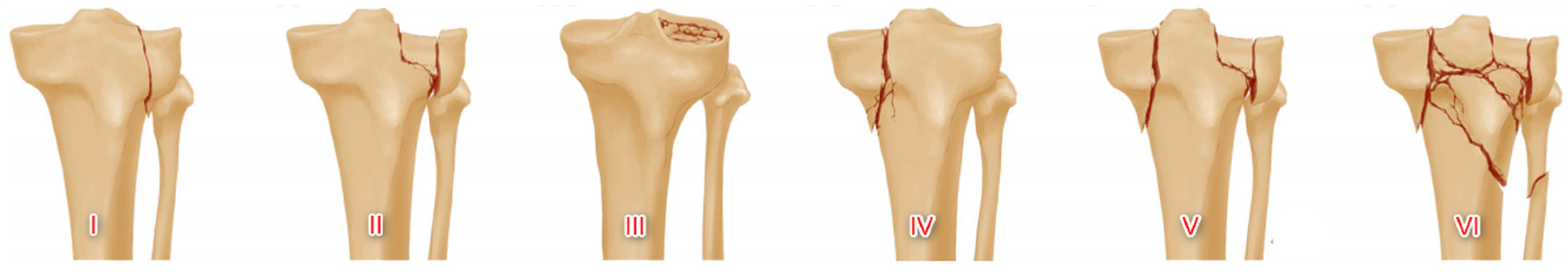
1.1. Schatzker Tibial Plateau Fracture Classification
1.2. Fracture Healing Process
- Proper blood supply through the nutrient artery (80%) and periosteal vessels (20%), which triggers the release of growth factors, stimulates local angiogenesis (which is another key process in bone healing [3]), vasodilation and ultimately, formation of new bone tissue. It has been shown [4] that blood supply not only provides nutrients but is also a source of mesenchymal stem cells that ultimately differentiate into osteoblasts. It is known that metaphyseal bone section heals significantly faster than diaphyseal bone because of a more intense vascularization of the first.
- Mechanical stability of the fracture. Relative displacement of bone fragments interrupts the development of new bone tissue and may cause malunion.
- (1)
- Primary healing occurs when the bone fragments are rigidly fixed in correct anatomic position with no gap in between [5]. Primary healing consists of remodeling of lamellar bone, the Haversian canals and the blood vessels without callus formation. The process can last from months to years.
- (2)
- If a gap of less than 0.01 mm the healing mechanism—contact healing—is slightly different. In this case, cutting cones, consisting of osteoclasts from across the sides of the fracture line, generate cavities at a rate of 50–100 μm/day, which subsequently are filled up with the Haversian system and osteoblasts lay down new bone tissue. Cutting cone mechanism occurs in diaphysis region of the bone (cortical tissue) and not in metaphysis region (such as tibial plateau).
- (3)
- In fractures with larger gaps (0.8–1 mm) the fracture region is filled by osteoclasts and then by lamellar bone orthogonal to the axis of the bone. The process is known as gap healing.
- (4)
- Secondary healing consists of endochondral ossification (which is one of the two fundamental mechanisms of bone tissue formation during fetal development of the mammalian skeletal system) and is the healing process most frequently encountered. Secondary healing occurs in cases where fracture is treated using orthopedic cast, or external or internal fixation.
1.3. Implant Device Effect on Fracture Healing Process
1.4. Common Orthopedic Implant Devices, Materials and Biomechanical Characterization
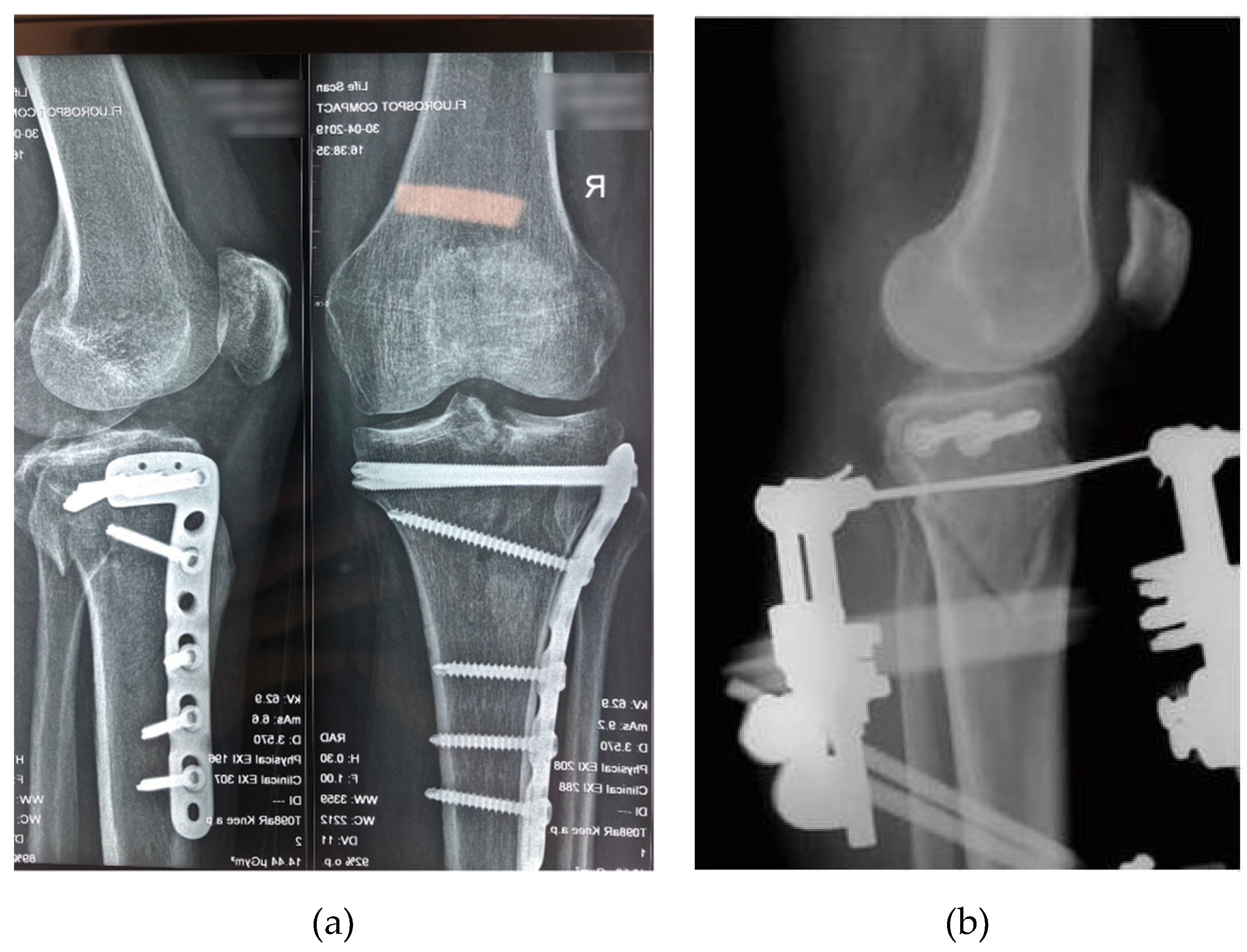
- Internal fixation (Figure 2a), which restores bone physiology and enable early mobilization of the limb. The function of the injured bones can be restored and full support for physiological load is ensured by applying internal fixation. The vast majority of internal fixation systems are manufactured from stainless steel or titanium. A review of internal fixation systems and the fracture sites for which they are suitable can be found in [18] and [19]. By means of internal fixation, malunion is a very rare occurrence and mobilization of the patient is very fast. Internal fixation systems have disadvantages, however. The stiffness and Young modulus of the implant material are much higher than in the case of cortical tissue of the human bone. Fixation of the bone fragments with high rigidity materials prevents load transfer to the healing bone, which is unfavorable for fracture callus remodeling [20]. The necessity of surgical removal after the bone healing is another trauma the patient has to undergo.
- External fixation (Figure 2b) is considered flexible fixation. External fixator systems consist of elements such as pins, wires (Schanz screws, Steinman pins, Kirschner wires) and belts that are conventionally used as a dynamic fixation of fractured bones. External fixation approach is used for open fractures with massive soft-tissue injuries such as open Type II, Type III fractures (Type II and III are open fractures with a soft tissue laceration larger than 1 cm and 10 cm respectively, minor and severe comminution respectively and with simple and complex fracture pattern, respectively) and even in articular fractures, in which the surgical trauma to the limb during fixation is reduced [18].
1.5. Objectives of the Study
- Investigate experimentally the correlation between the compressive force applied axially to a bio-mechanical system bone—implant device and the deformation of the implant.
- Develop an MLA model that is capable of predicting the implant deformation as a function of applied force and implant type.
- Establish if in case of similar mechanical stress, different types of implant devices perform significantly different (in a statistical sense) in terms of micromovement at the fracture site.
2. Materials and Methods
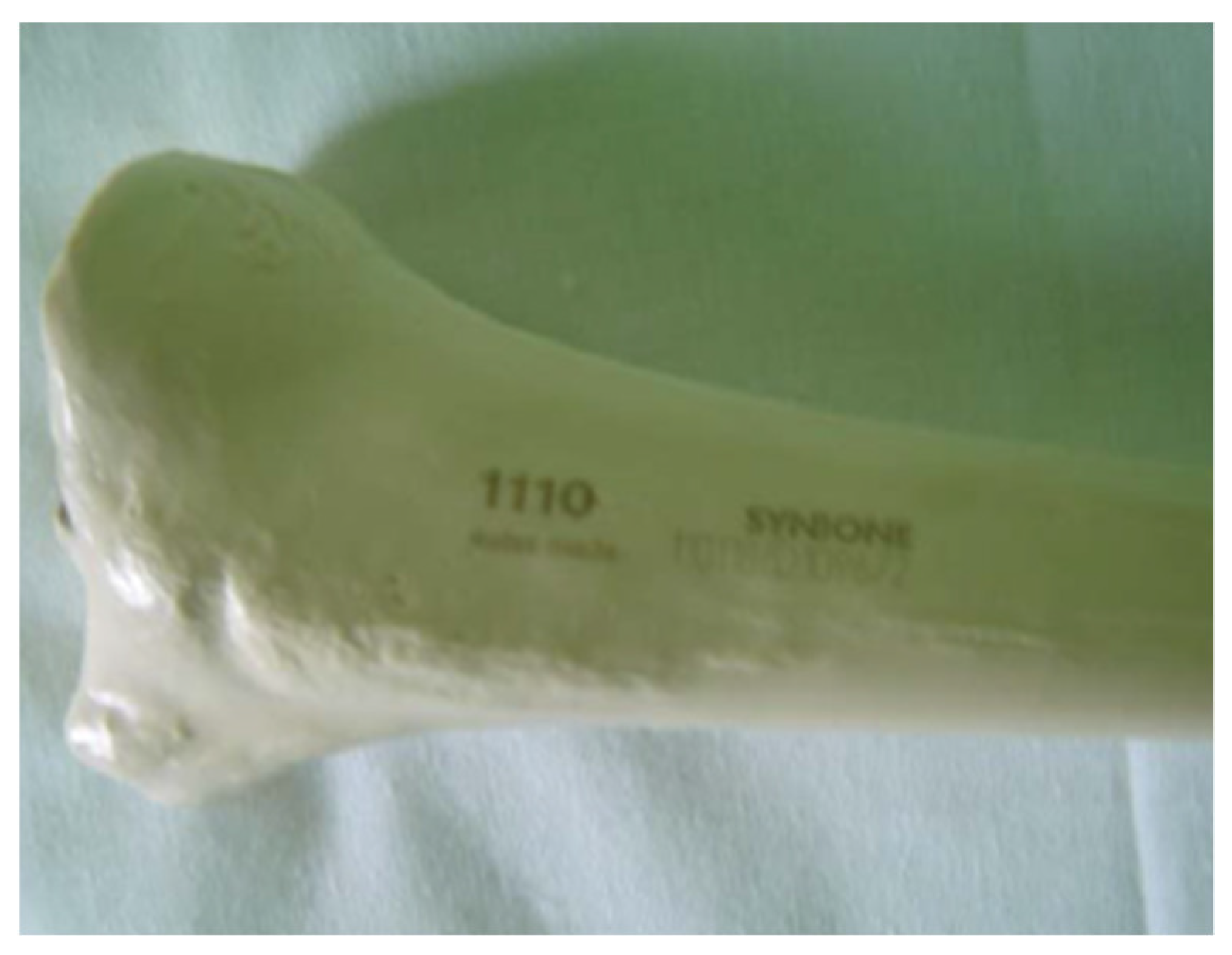
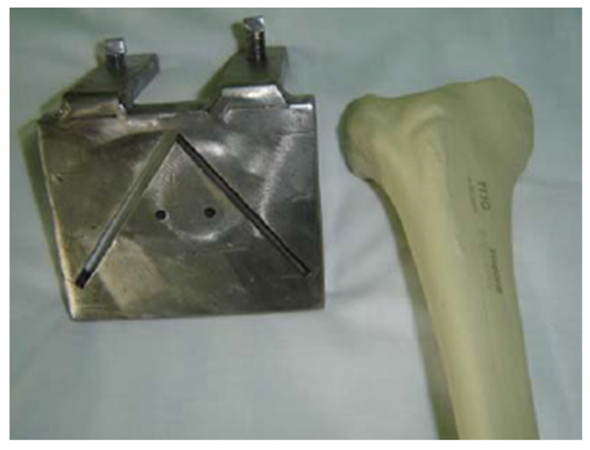
2.1. Bone Model
2.2. Implant Devices
2.3. Fracture Stabilization Techniques and Implant Devices
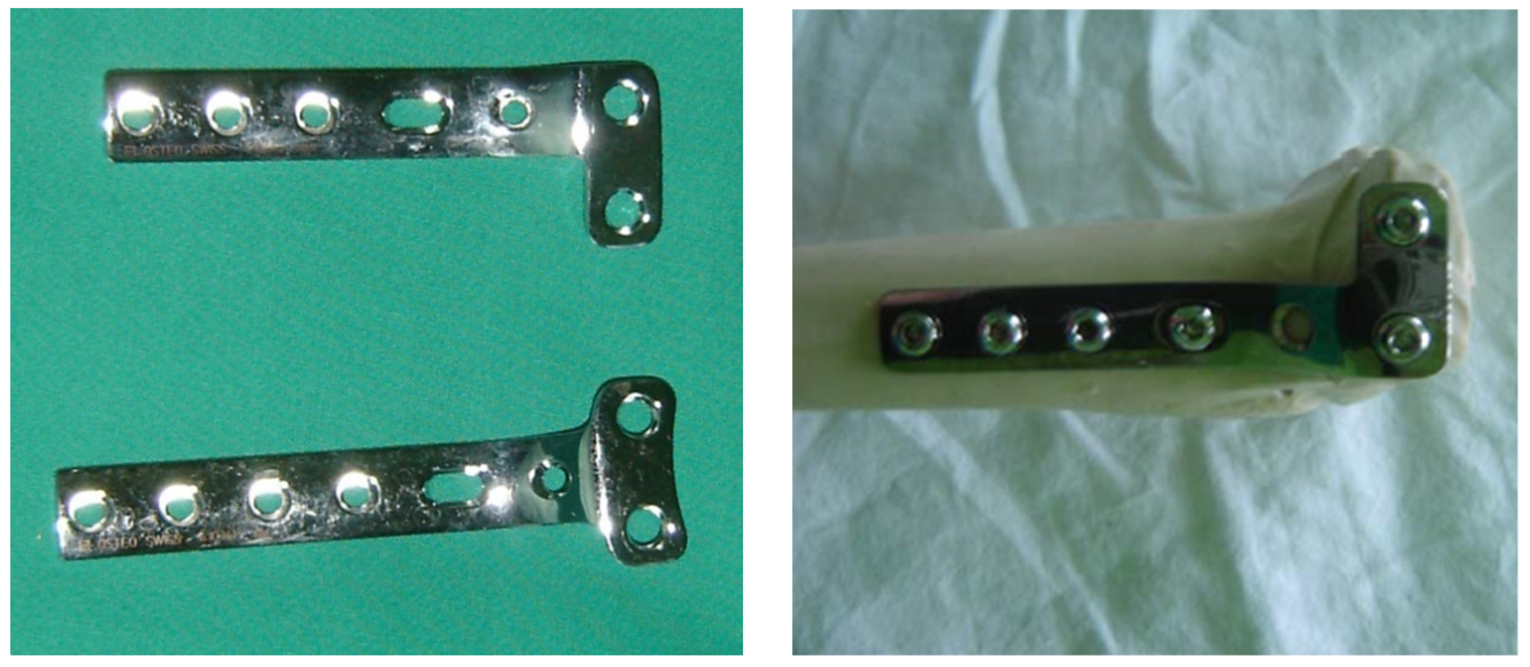
2.3.1. L Plate
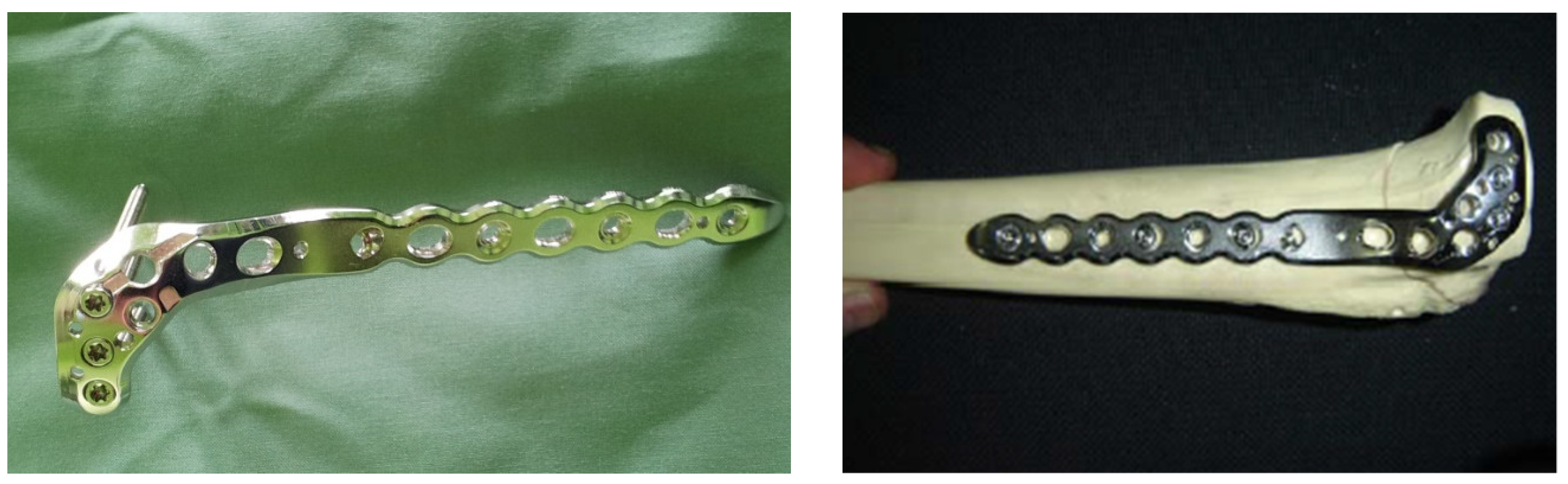
2.3.2. PLS Plate
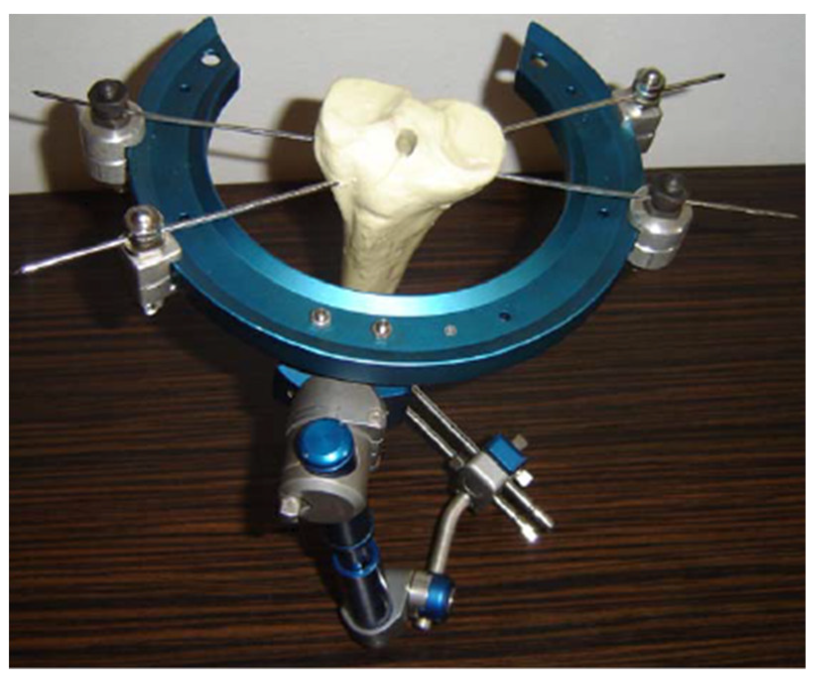
2.3.3. Hybrid External Fixator
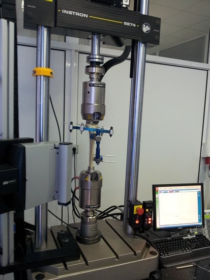
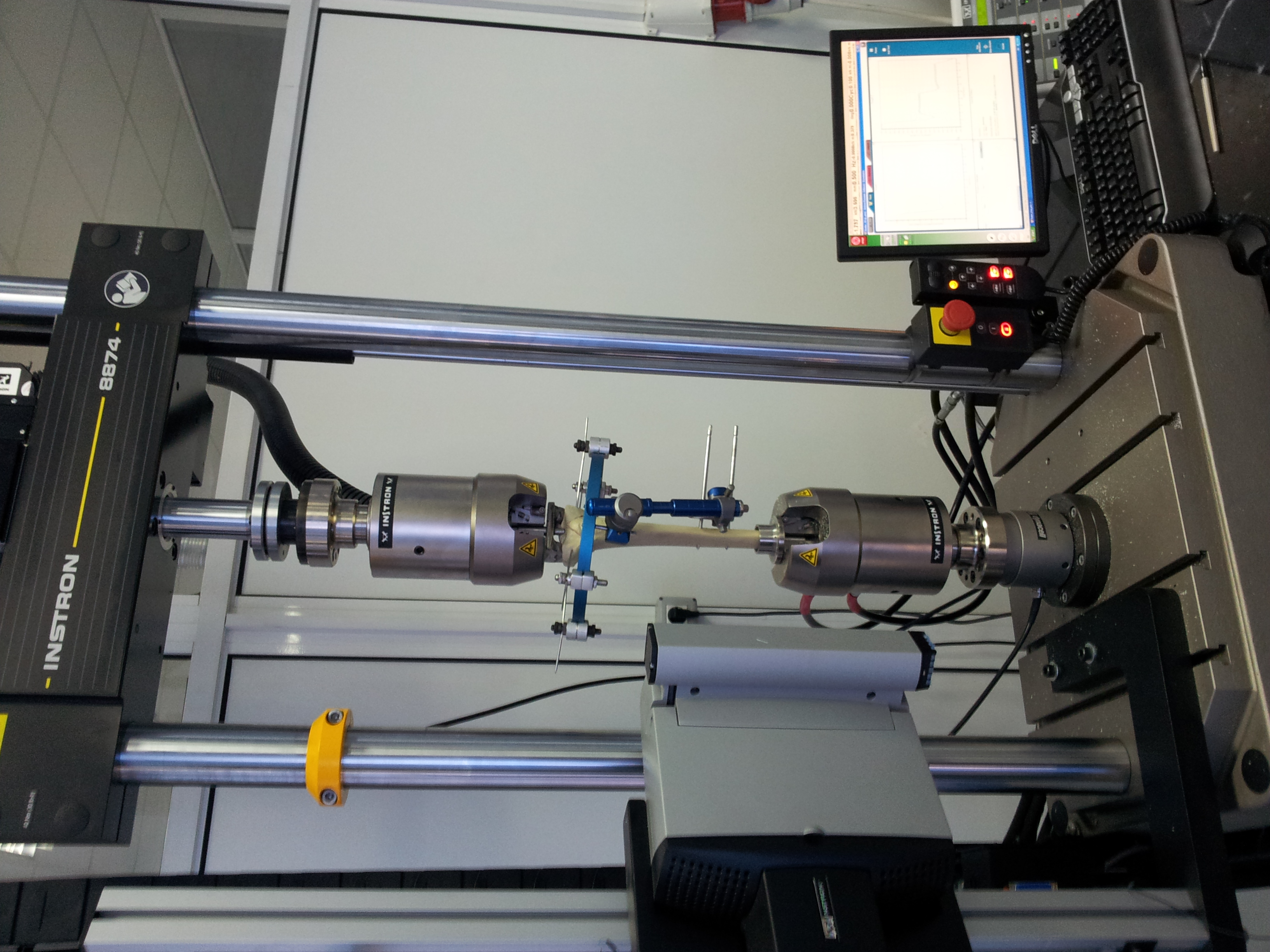
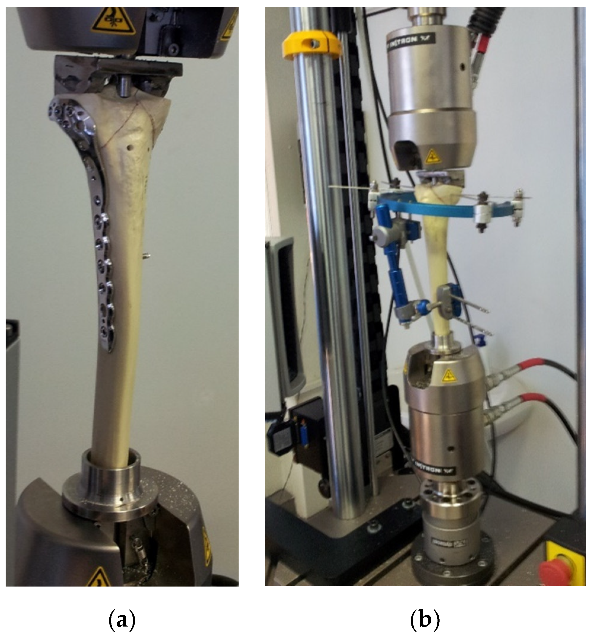
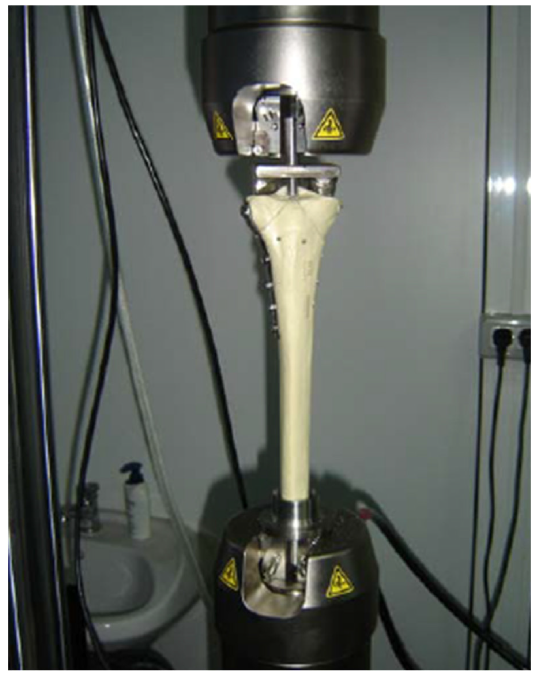
2.4. Test Machine and Assembly
2.5. Preparation of the Bone Model
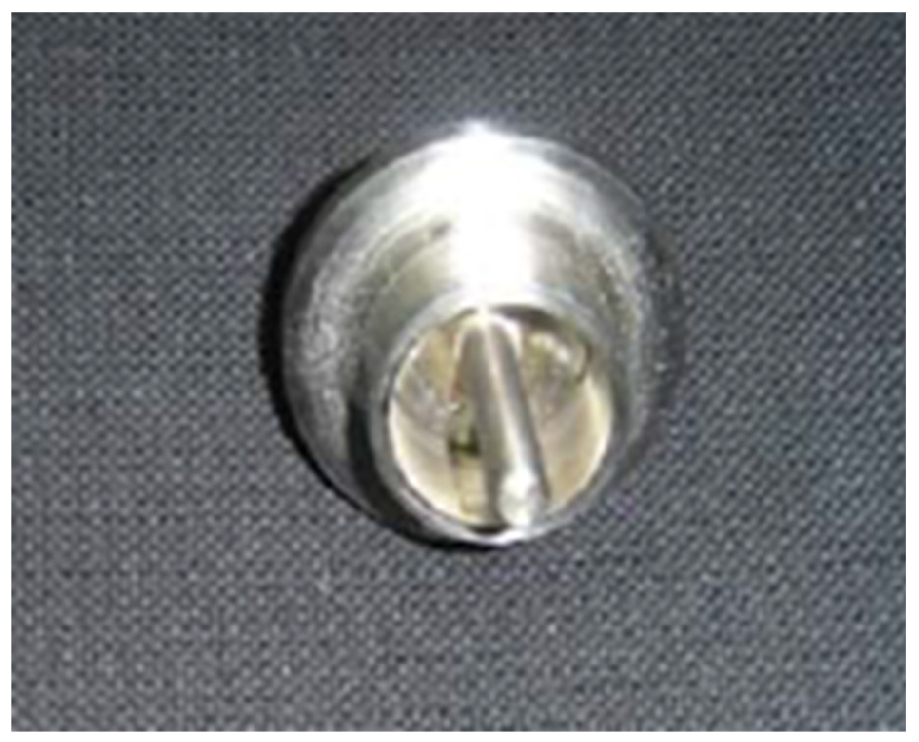
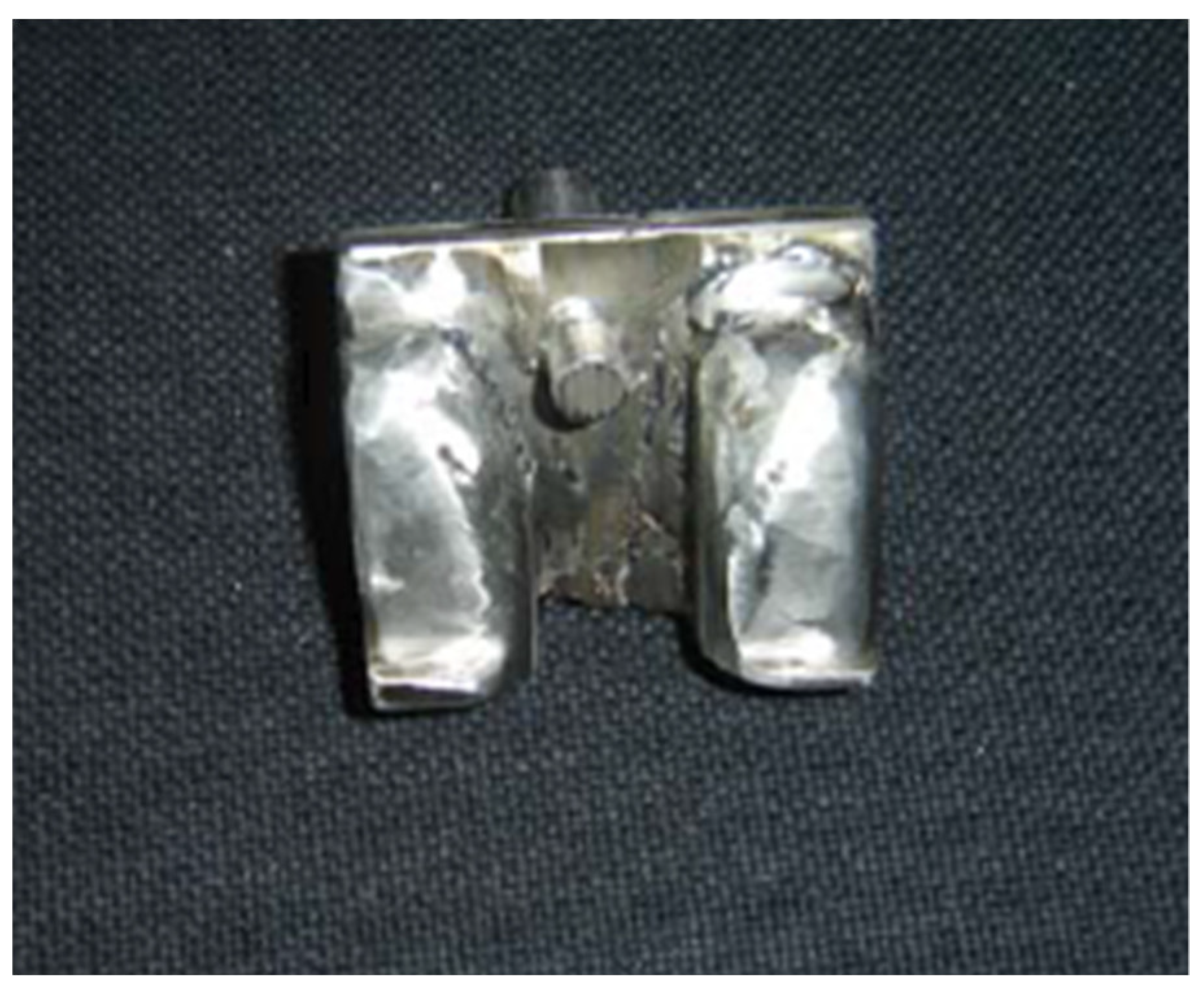
2.6. Bone—Implant Device Model Fastening System
3. Results
3.1. Test Procedure
- Group 1. 15 bone models with L plate implant
- Group 2. 15 bone models with PLS plate implant
- Group 3. 15 bone models with hybrid external fixator implant
3.2. Preliminary Processing of the Raw Data
3.3. Development of the Artificial Neural Network (ANN) Model
- Bone tissue is a material with complex mechanical properties, significantly different from those of the implant device (Young modulus highly anisotropic [50], shear and bulk modulus, elastic limit, homogeneity, and isotropy).
- Screw assembly between the bone and the implant introduces complex effects that cannot be fully accounted for analytically. Load is transferred between bone and implant device by means of screws, which undergo complex stresses, especially bending and shear. A complex stress field occurs in the bone tissue in the vicinity of the screw insertion region.
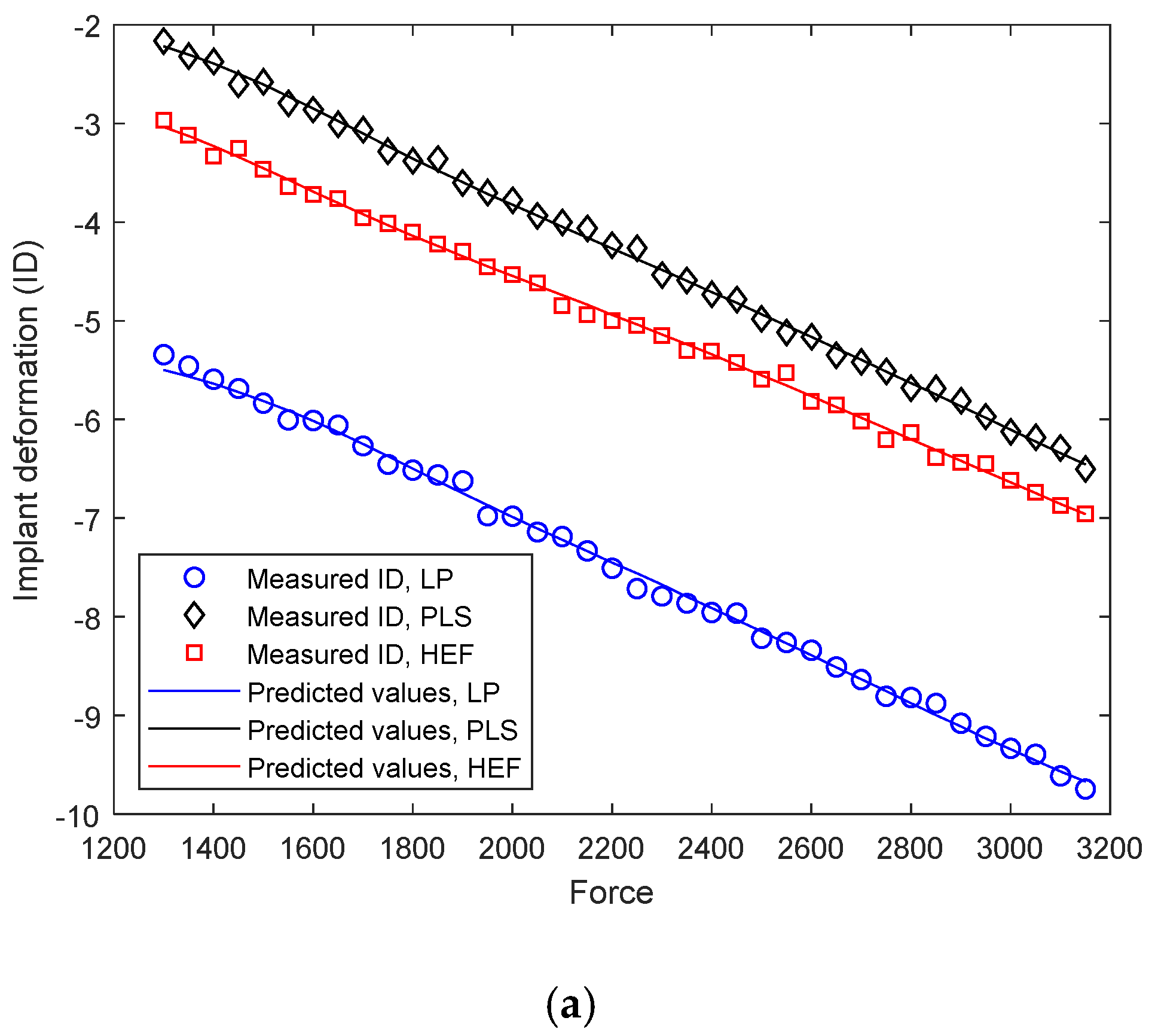
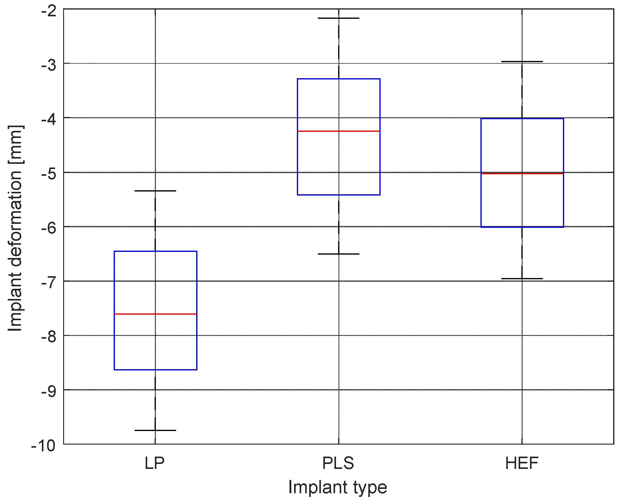
- L plate and PLS plate devices are somewhat similar regarding the implant deformation under load. However, the HEF is different in many aspects from the first two. On the other hand, PLS plate and HEF perform similarly from a mechanical point of view with the difference that PLS is an internal fixator, requiring open surgery while HEF is a minimally invasive implanting technique.
- Although standard implant insertion surgical procedures are in place, minor differences in terms of screw position, anatomic particularities of the bone, fracture particularities, surgeon experience and preferences and several other factors introduce a random component of the bio-mechanical behavior of the implant device—bone system.
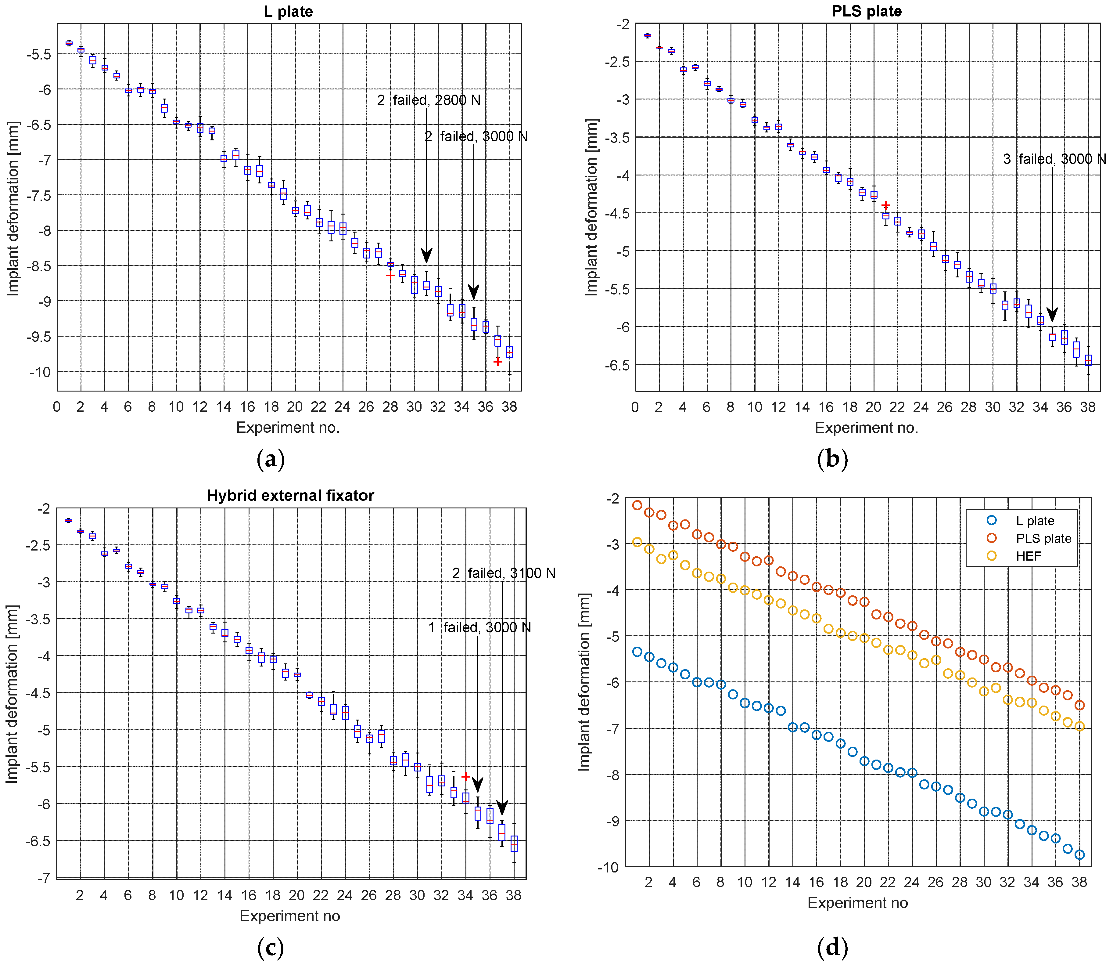
- It appears from Figure 12a–c that the standard deviation (scattering of data points around mean value) tends to increase as the applied force increases. This is a clear indication that random factors with varying influence exist.
- Every class must be represented. The training data usually consists of several possible subgroups, each with its own central tendency toward a particular pattern. All such patterns must be presented to the ANN model during the training stage.
- Within each class, statistical variation must be adequately represented by including the relevant noise effects.
4. Discussion
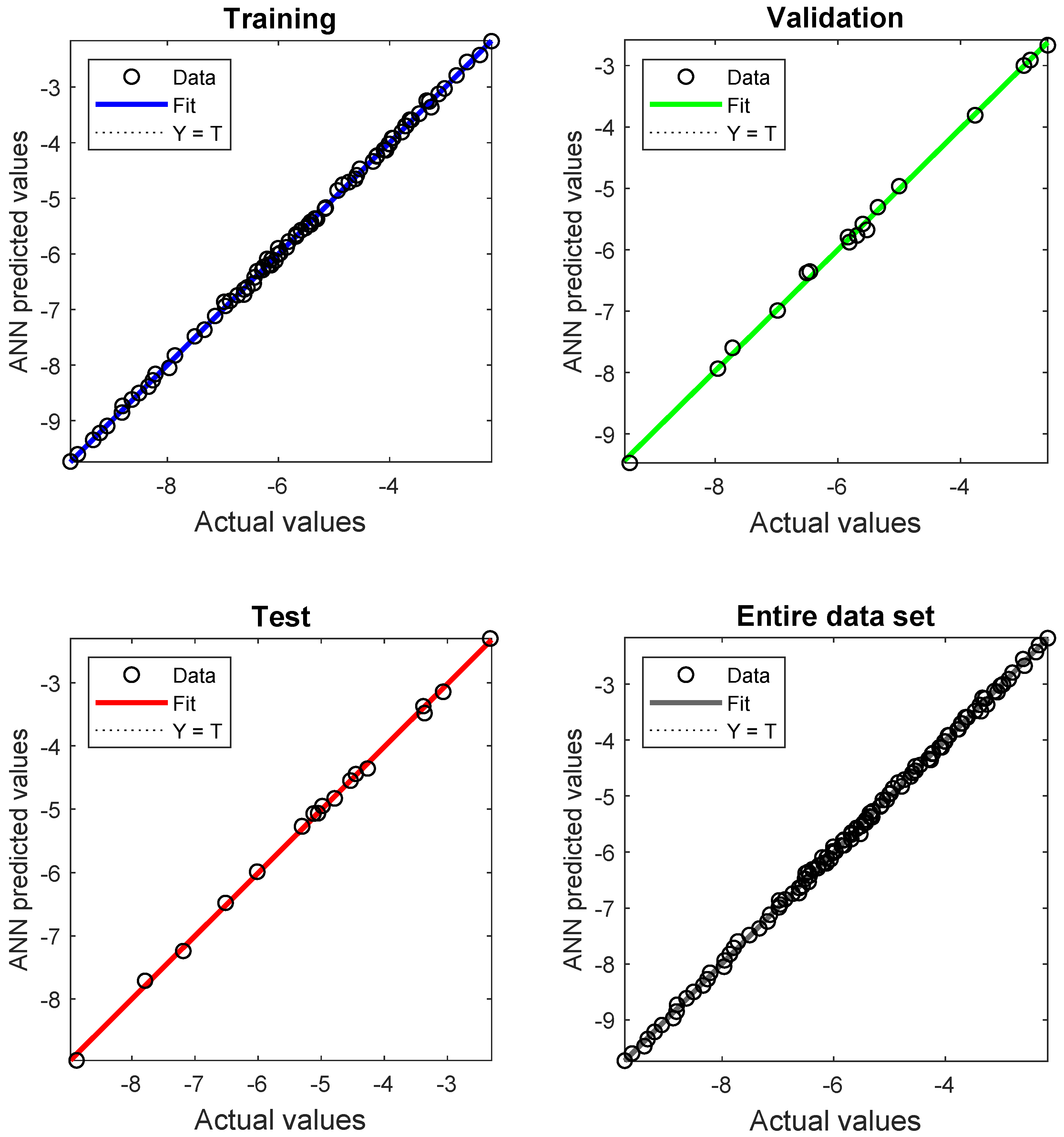
4.1. ANN Model Results and Performance
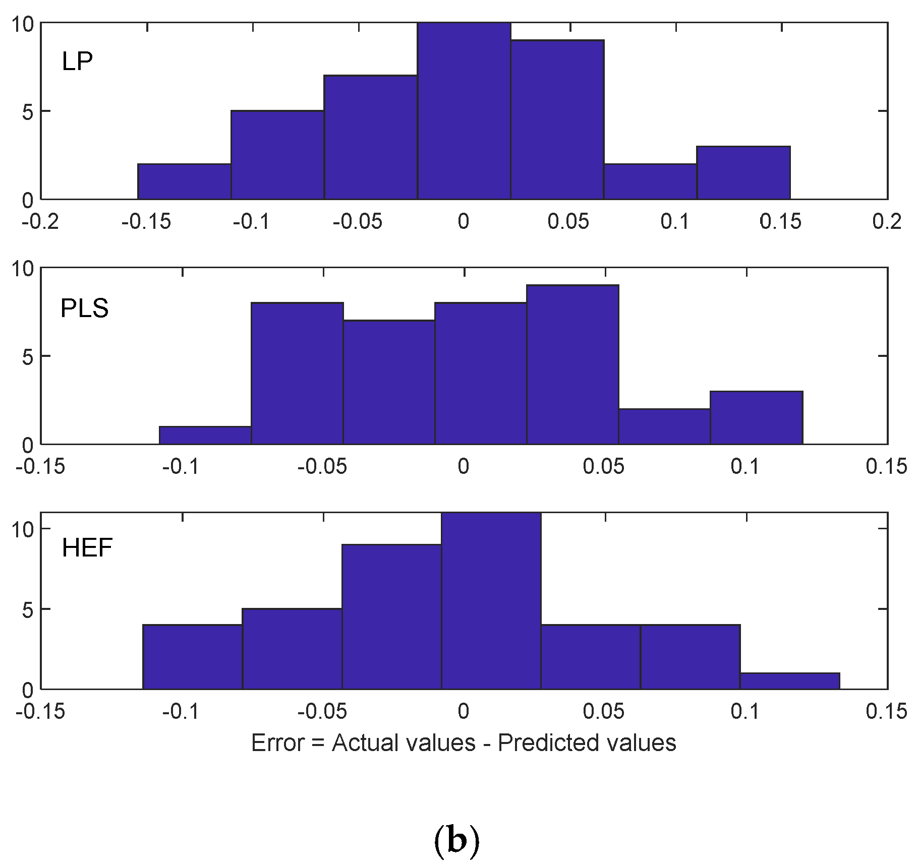
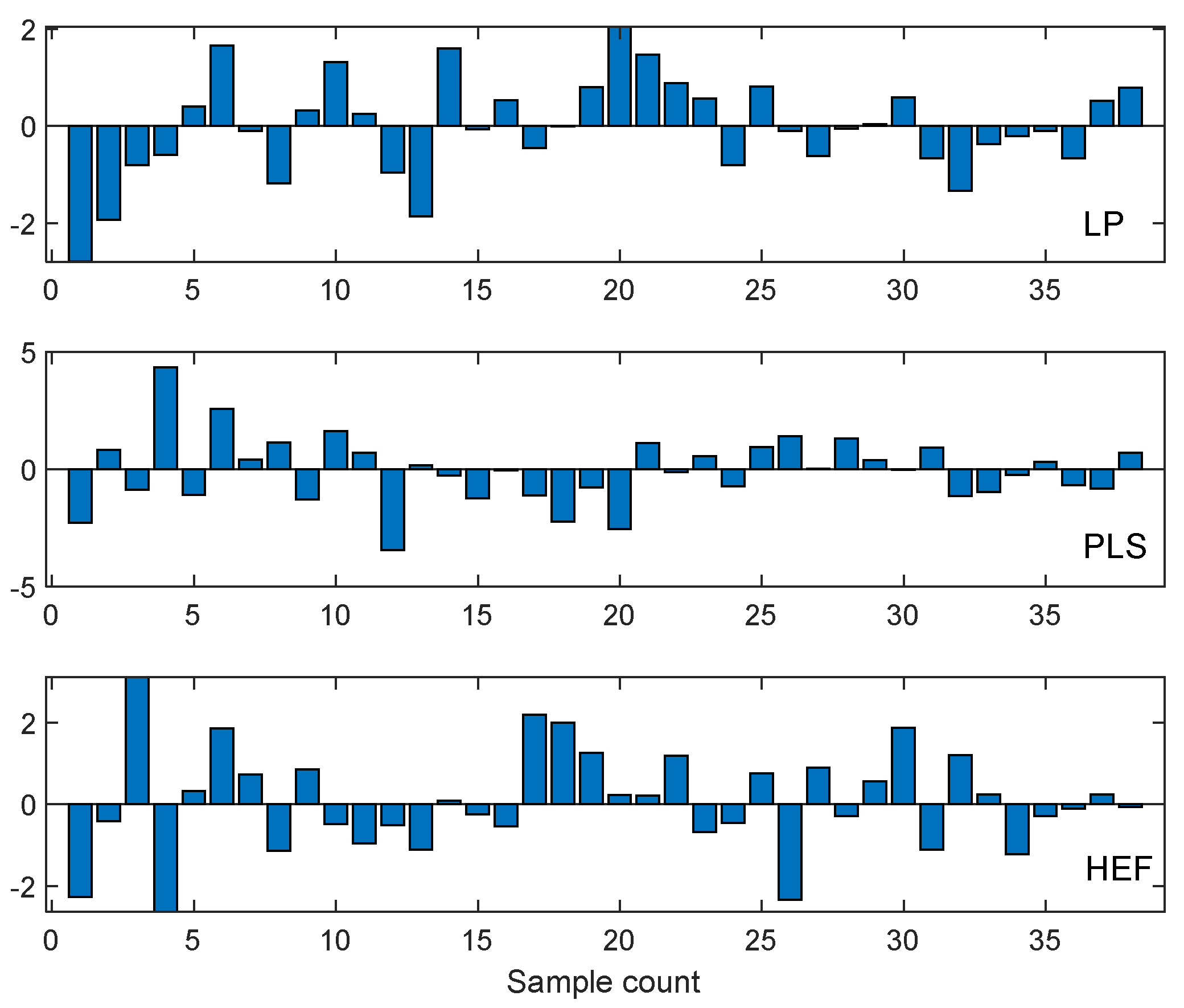
4.2. Differential Analysis of Implant Deformation Data
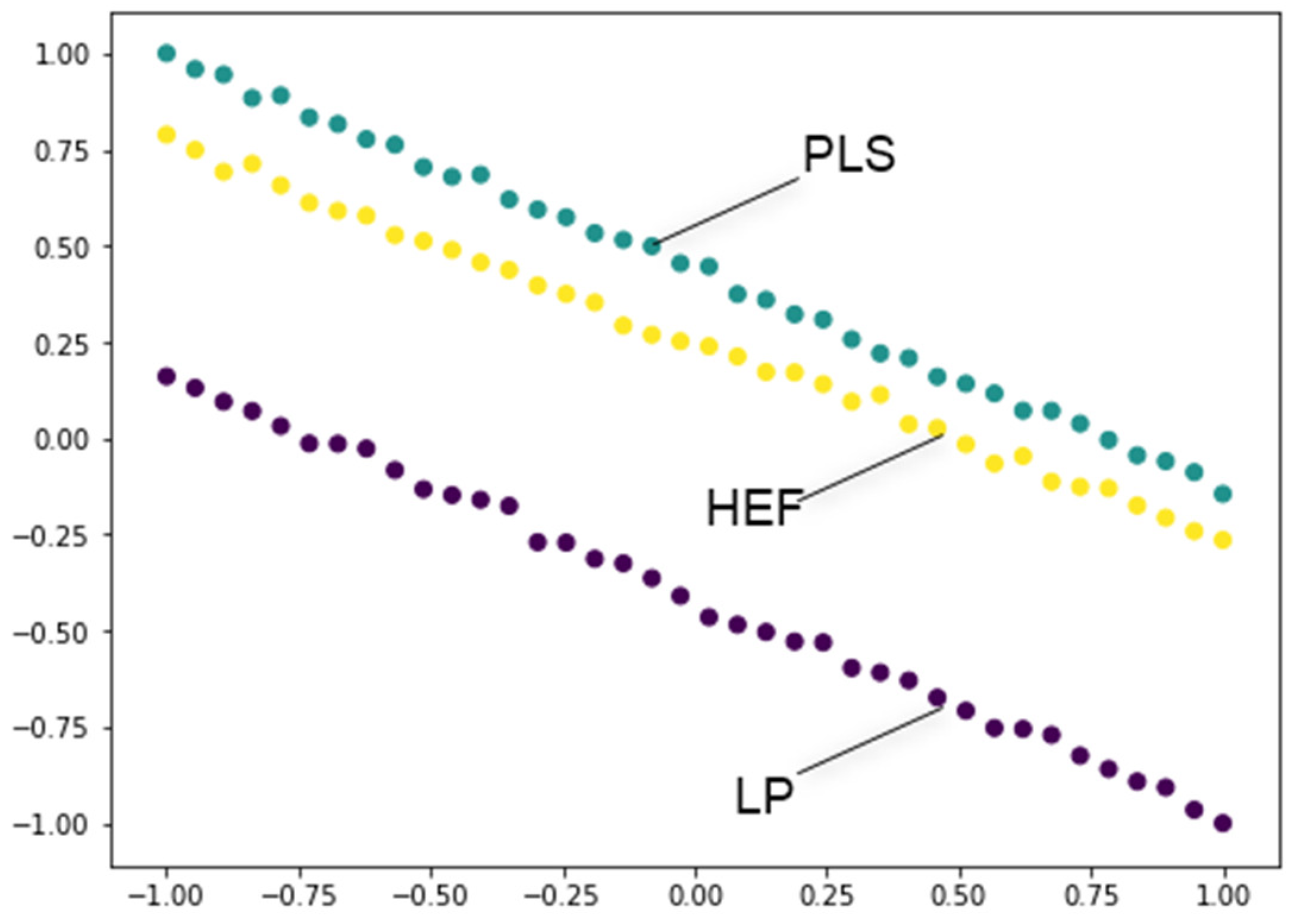
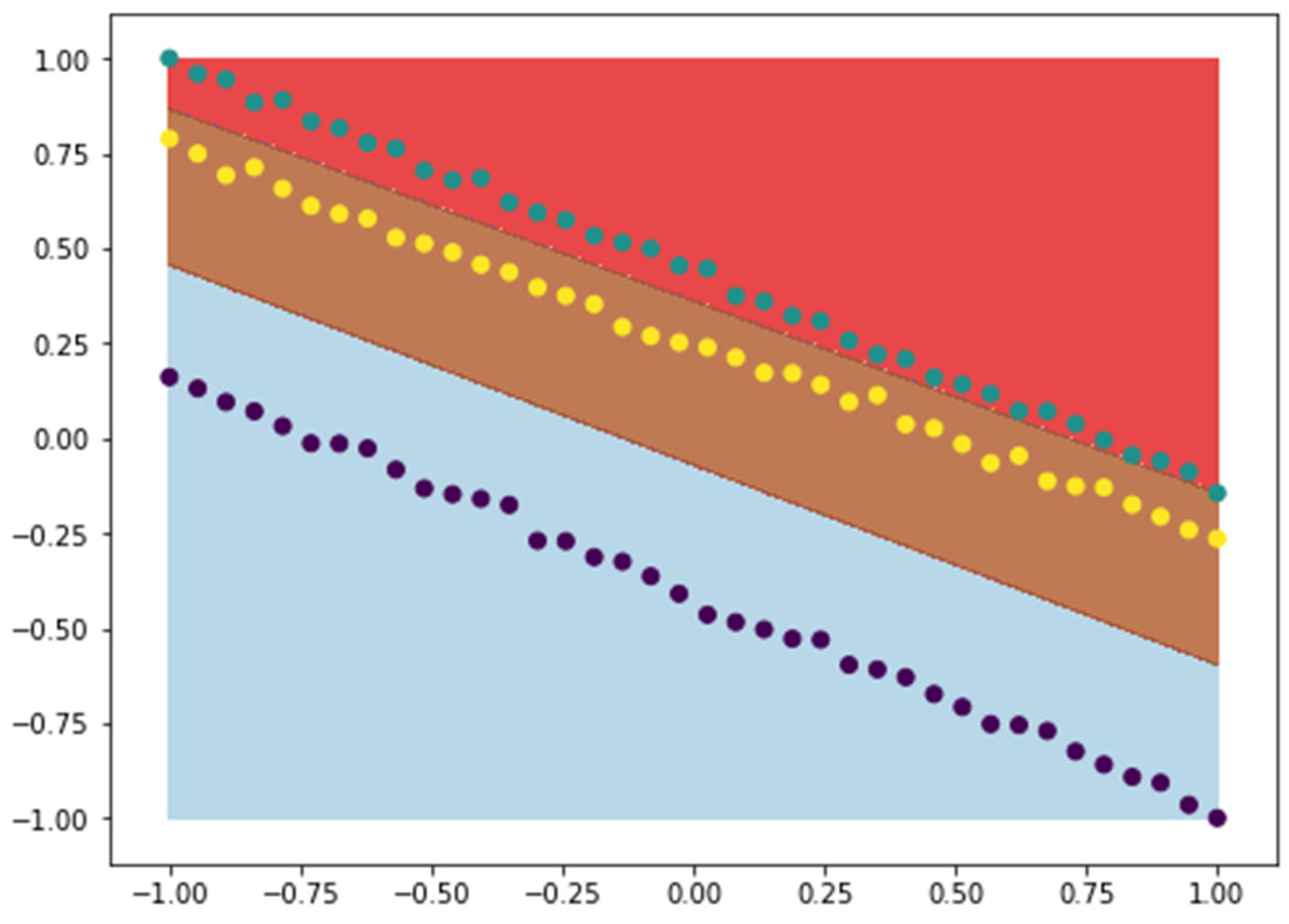
4.3. Application of SVM Classification to Implant Deformation Data
5. Conclusions
Author Contributions
Funding
Conflicts of Interest
References
- Kfuri, M.; Schatzker, J. Revisiting the Schatzker classification of tibial plateau fractures. Injury 2018, 49, 2252–2263. [Google Scholar] [CrossRef] [PubMed]
- Oryan, A.; Monazzah, S.; Bigham-Sadegh, A. Bone Injury and Fracture Healing Biology. Biomed. Environ. Sci. 2015, 28, 57–71. [Google Scholar]
- Saran, U.; Piperni, S.G.; Chatterjee, S. Role of angiogenesis in bone repair. Arch. Biochem. Biophys. 2014, 561, 109–117. [Google Scholar] [CrossRef] [PubMed]
- Fayaz, H.C.; Giannoudis, P.V.; Vrahas, M.S.; Smith, R.M.; Moran, C.; Pape, H.C.; Krettek, C.; Jupiter, J.B. The role of stem cells in fracture healing and nonunion. Int. Orthop. SICOT 2011, 35, 1587–1597. [Google Scholar] [CrossRef] [PubMed]
- McKibbin, B. The biology of fracture healing in long bones. J. Bone Jt. Surgery. Br. Vol. 1978, 60, 150–162. [Google Scholar] [CrossRef]
- Olivares-Navarrete, R.; Gittens, R.A.; Schneider, J.M.; Hyzy, S.L.; Haithcock, D.A.; Ullrich, P.F.; Schwartz, Z.; Boyan, B.D. Osteoblasts exhibit a more differentiated phenotype and increased bone morphogenetic protein production on titanium alloy substrates than on poly-ether-ether-ketone. Spine J. 2012, 12, 265–272. [Google Scholar] [CrossRef]
- Krettek, C.; Schandelmaier, P.; Miclau, T.; Bertram, R.; Holmes, W.; Tscherne, H. Transarticular joint reconstruction and indirect plate osteosynthesis for complex distal supracondylar femoral fractures. Injury 1997, 28, A31–A41. [Google Scholar] [CrossRef]
- Hente, R.; Füchtmeier, B.; Schlegel, U.; Ernstberger, A.; Perren, S.M. The influence of cyclic compression and distraction on the healing of experimental tibial fractures. J. Orthop. Res. 2004, 22, 709–715. [Google Scholar] [CrossRef]
- Claes, E.L.; Heigele, C.A.; Neidlinger-Wilke, C.; Kaspar, D.; Seidl, W.; Margevicius, K.; Augat, P. Effects of Mechanical Factors on the Fracture Healing Process. Clin. Orthop. Relat. Res. 1998, 355, S132–S147. [Google Scholar] [CrossRef]
- Gittens, R.A.; Olivares-Navarrete, R.; Schwartz, Z.; Boyan, B. Implant osseointegration and the role of microroughness and nanostructures: Lessons for spine implants. Acta Biomater. 2014, 10, 3363–3371. [Google Scholar] [CrossRef]
- Loi, F.; Córdova, L.A.; Pajarinen, J.; Lin, T.; Yao, Z.; Goodman, S.B. Inflammation, fracture and bone repair. Bone 2016, 86, 119–130. [Google Scholar] [CrossRef] [PubMed]
- Li, L.; Yang, S.; Xu, L.; Li, Y.; Fu, Y.; Zhang, H.; Song, J. Nanotopography on titanium promotes osteogenesis via autophagymediated signaling between YAP and β-catenin. Acta Biomater. 2019, 96, 674–685. [Google Scholar] [CrossRef] [PubMed]
- Gao, P.; Fan, B.; Yu, X.; Liu, W.; Wu, J.; Shi, L.; Yang, D.; Tan, L.; Wan, P.; Hao, Y.; et al. Biofunctional magnesium coated Ti6Al4V scaffold enhances osteogenesis and angiogenesis in vitro and in vivo for orthopedic application. Bioact. Mater. 2020, 5, 680–693. [Google Scholar] [CrossRef] [PubMed]
- Jia, L.; Han, F.; Wang, H.; Zhu, C.; Guo, Q.; Li, J.; Zhao, Z.; Zhang, Q.; Zhu, X.; Li, B. Polydopamine-assisted surface modification for orthopaedic implants. J. Orthop. Transl. 2019, 17, 82–95. [Google Scholar] [CrossRef]
- Niinomi, M.; Nakai, M. Titanium-Based Biomaterials for Preventing Stress Shielding between Implant Devices and Bone. Int. J. Biomater. 2011, 2011, 1–10. [Google Scholar] [CrossRef] [PubMed]
- Song, Y.; Xu, D.S.; Yang, R.; Li, D.; Wu, W.T.; Guo, Z.X. Theoretical study of the effects of alloying elements on the strength and modulus of β-type bio-titanium alloys. Mater. Sci. Eng. A 1999, 260, 269–274. [Google Scholar] [CrossRef]
- Tian, L.; Tang, N.; Ngai, T.; Wu, C.; Ruan, Y.C.; Huang, L.; Qin, L. Hybrid fracture fixation systems developed for orthopaedic applications: A general review. J. Orthop. Transl. 2018, 16, 1–13. [Google Scholar] [CrossRef]
- Taljanovic, M.S.; Jones, M.D.; Ruth, J.T.; Benjamin, J.B.; Sheppard, J.E.; Hunter, T.B. Fracture Fixation. Radiographics 2003, 23, 1569–1590. [Google Scholar] [CrossRef]
- Chris Colton, S.K. AO Surgery Reference, 1st ed.; AO Foundation: Biel, Switzerland, 2017. [Google Scholar]
- Hayes, J.S.; Richards, R.G. The use of titanium and stainless steel in fracture fixation. Expert Rev. Med. Devices 2010, 7, 843–853. [Google Scholar] [CrossRef]
- Uhthoff, H.K.; Poitras, P.; Backman, D.S. Internal plate fixation of fractures: Short history and recent developments. J. Orthop. Sci. 2006, 11, 118–126. [Google Scholar] [CrossRef]
- Greenhagen, R.M.; Johnson, A.R.; Joseph, A. Internal Fixation: A Historical Review. Clin. Podiatr. Med. Surg. 2011, 28, 607–618. [Google Scholar] [CrossRef] [PubMed]
- Frigg, R. Locking Compression Plate (LCP). An osteosynthesis plate based on the Dynamic Compression Plate and the Point Contact Fixator (PC-Fix). Injury 2001, 32, 63–66. [Google Scholar] [CrossRef]
- Campbell, S.T.; Goodnough, L.H.; Salazar, B.; Lucas, J.F.; Bishop, J.A.; Gardner, M.J. How do pilon fractures heal? An analysis of dual plating and bridging callus formation. Injury 2020, 51, 1655–1661. [Google Scholar] [CrossRef] [PubMed]
- Gao, X.; Fraulob, M.; Haïat, G. Biomechanical behaviours of the bone–implant interface: A review. J. R. Soc. Interface 2019, 16, 20190259. [Google Scholar] [CrossRef] [PubMed]
- Duyck, J.; Vandamme, K.; Geris, L.; Van Oosterwyck, H.; De Cooman, M.; Vandersloten, J.; Puers, R.; Naert, I. The influence of micro-motion on the tissue differentiation around immediately loaded cylindrical turned titanium implants. Arch. Oral Biol. 2006, 51, 1–9. [Google Scholar] [CrossRef] [PubMed]
- Taylor, M.; Barrett, D.S.; Deffenbaugh, D. Influence of loading and activity on the primary stability of cementless tibial trays. J. Orthop. Res. 2012, 30, 1362–1368. [Google Scholar] [CrossRef]
- Fukuoka, S.; Yoshida, K.; Yamano, Y. Estimation of the migration of tibial components in total knee arthroplasty: A roentgen stereophotogrammetric analysis. J. Bone Jt. Surgery. Br. Vol. 2000, 82, 222–227. [Google Scholar] [CrossRef]
- Shirazi-Adl, A. Finite Element Stress Analysis of a Push-Out Test Part 1: Fixed Interface Using Stress Compatible Elements. J. Biomech. Eng. 1992, 114, 111–118. [Google Scholar] [CrossRef]
- Yamaji, T.; Ando, K.; Wolf, S.; Augat, P.; Claes, L. The effect of micromovement on callus formation. J. Orthop. Sci. 2001, 6, 571–575. [Google Scholar] [CrossRef]
- Kenwright, J.; Goodship, A.; Kelly, D.; Newman, J.; Harris, J.; Richardson, J.; Evans, M.; Spriggins, A.; Burrough, S.; Rowley, D. Effect of controlled axial micromovement on healing of tibial fractures. Lancet 1986, 328, 1185–1187. [Google Scholar] [CrossRef]
- Gervais, B.; Vadean, A.; Raison, M.; Brochu, M. Failure analysis of a 316L stainless steel femoral orthopedic implant. Case Stud. Eng. Fail. Anal. 2016, 5–6, 30–38. [Google Scholar] [CrossRef]
- Wang, W.-C.; Chen, L.-B.; Chang, W.-J. Development and Experimental Evaluation of Machine-Learning Techniques for an Intelligent Hairy Scalp Detection System. Appl. Sci. 2018, 8, 853. [Google Scholar] [CrossRef]
- Miyagi, S.; Sugiyama, S.; Kozawa, K.; Moritani, S.; Sakamoto, S.-I.; Sakai, O. Classifying Dysphagic Swallowing Sounds with Support Vector Machines. Heal. 2020, 8, 103. [Google Scholar] [CrossRef] [PubMed]
- Merrill, R.K.; Ferrandino, R.M.; Hoffman, R.; Shaffer, G.W.; Ndu, A. Machine Learning Accurately Predicts Short-Term Outcomes Following Open Reduction and Internal Fixation of Ankle Fractures. J. Foot Ankle Surg. 2019, 58, 410–416. [Google Scholar] [CrossRef] [PubMed]
- Halilaj, E.; Rajagopal, A.; Fiterau, M.; Hicks, J.L.; Hastie, T.J.; Delp, S.L. Machine learning in human movement biomechanics: Best practices, common pitfalls, and new opportunities. J. Biomech. 2018, 81, 1–11. [Google Scholar] [CrossRef] [PubMed]
- Kang, Y.-J.; Yoo, J.-I.; Cha, Y.-H.; Park, C.H.; Kim, J.-T. Machine learning–based identification of hip arthroplasty designs. J. Orthop. Transl. 2020, 21, 13–17. [Google Scholar] [CrossRef]
- Pandey, R.K.; Panda, S. Predicting Temperature in Orthopaedic Drilling using Back Propagation Neural Network. Procedia Eng. 2013, 51, 676–682. [Google Scholar] [CrossRef][Green Version]
- Urban, G.; Porhemmat, S.; Stark, M.; Feeley, B.; Okada, K.; Baldi, P. Classifying shoulder implants in X-ray images using deep learning. Comput. Struct. Biotechnol. J. 2020, 18, 967–972. [Google Scholar] [CrossRef]
- Bhavsar, H.P.; Panchal, M.H. A Review on Support Vector Machine for Data Classification. Adv. Res. Comput. Eng. Technol. 2012, 1, 185–189. [Google Scholar]
- Battineni, G.; Chintalapudi, N.; Amenta, F. Machine learning in medicine: Performance calculation of dementia prediction by support vector machines (SVM). Informatics Med. Unlocked 2019, 16, 100200. [Google Scholar] [CrossRef]
- Yu, W.; Liu, T.; Valdez, R.; Gwinn, M.; Khoury, M.J. Application of support vector machine modeling for prediction of common diseases: The case of diabetes and pre-diabetes. BMC Med. Informatics Decis. Mak. 2010, 10, 16. [Google Scholar] [CrossRef]
- Janardhanan, P.; Sabika, F. Effectiveness of Support Vector Machines in Medical Data mining. J. Commun. Softw. Syst. 2015, 11, 25. [Google Scholar] [CrossRef]
- Jiang, Y.; Li, Z.; Zhang, L.; Sun, P. An Improved SVM Classifier for Medical Image Classification. In Computer Vision; Rough Sets and Intelligent Systems Paradigms. RSEISP 2007. Lecture Notes in Computer Science; Kryszkiewicz, M., Peters, J.F., Rybinski, H., Skowron, A., Eds.; Springer Science and Business Media LLC: Berlin/Heidelberg, Germany, 2007; Volume 4585. [Google Scholar]
- Acevedo, J.I.; Sammarco, V.J.; Boucher, H.R.; Parks, B.G.; Schon, L.C.; Myerson, M.S. Mechanical comparison of cyclic loading in five different first metatarsal shaft osteotomies. Foot Ankle Int. 2002, 23, 711–716. [Google Scholar] [CrossRef] [PubMed]
- Gefen, A.; Seliktar, R. Comparison of the trabecular architecture and the isostatic stress flow in the human calcaneus. Med. Eng. Phys. 2004, 26, 119–129. [Google Scholar] [CrossRef] [PubMed]
- Lin, P.P.; Roe, S.; Kay, M.; Abrams, C.F.; Jones, A. Placement of screws in the sustentaculum tali. A calcaneal fracture model. Clin. Orthop. Relat. Res. 1998, 352, 194–201. [Google Scholar] [CrossRef]
- Mohamad, W.M.; Selamat, M.Z.; Bundjali, B.; Musa, M.; Dom, H.M. Corrosion analysis of the cold work 316L stainless steel in simulated body fluids. In Proceedings of the Mechanical Engineering Research Day 2016, Melaka, Malaysia, 31 March 2016; Centre for Advanced Research on Energy: Melaka, Malaysia, 2016; pp. 149–150. [Google Scholar]
- Subit, D.; Arregui, C.; Salzar, R.; Crandall, J. Pediatric, Adult and Elderly Bone Material Properties. In Proceedings of the IRCOBI Conference 2013, Gothenburg, Sweden, 11–13 September 2013. [Google Scholar]
- Hoffmeister, B.K.; Smith, S.R.; Handley, S.M.; Rho, J.Y. Anisotropy of Young’s modulus of human tibial cortical bone. Med. Biol. Eng. Comput. 2000, 38, 333–338. [Google Scholar] [CrossRef]
- Faur, C.I.; Niculescu, B. Comparative biomechanical analysis of three implants used in bicondylar tibial fractures. Wien. Med. Wochenschr. 2017, 138, 94. [Google Scholar] [CrossRef] [PubMed]


| Density | Tensile Strength (min) | Elastic Modulus | Hardness | |
|---|---|---|---|---|
| Rockwell B | Brinell | |||
| 8000 kg/m3 | 485 MPa | 193 GPa | 95 | 217 |
| Implant Type | Correlation Coefficient | |
|---|---|---|
| Pearson | Spearman | |
| L plate | −0.9989 | −1.0000 |
| PLS plate | −0.9993 | −0.9996 |
| Hybrid external fixator | −0.9988 | −0.9993 |
| Data Set | Number of Samples | Mean Square Error | Pearson Correlation Coefficient |
|---|---|---|---|
| Training | 80 | 3.218E-3 | 0.9995 |
| Validation | 17 | 6.330E-3 | 0.9902 |
| Testing | 17 | 2.738E-3 | 0.9852 |
| Data Set | Line Parameters | |
|---|---|---|
| Slope | Intercept | |
| Training | 1.0025 | 0.0023 |
| Validation | 0.9960 | 0.0791 |
| Test | 1.0018 | 0.0352 |
| Entire data set | 1.0087 | 0.0192 |
| Implant Type | Mean | Mean (Absolute Values) | Standard Deviation |
|---|---|---|---|
| LP | 0.0228 | 0.0568 | 0.0423 |
| PLS | 0.154 | 0.0421 | 0.0307 |
| HEF | −0.158 | 0.0450 | 0.0345 |
© 2020 by the authors. Licensee MDPI, Basel, Switzerland. This article is an open access article distributed under the terms and conditions of the Creative Commons Attribution (CC BY) license (http://creativecommons.org/licenses/by/4.0/).
Share and Cite
Niculescu, B.; Faur, C.I.; Tataru, T.; Diaconu, B.M.; Cruceru, M. Investigation of Biomechanical Characteristics of Orthopedic Implants for Tibial Plateau Fractures by Means of Deep Learning and Support Vector Machine Classification. Appl. Sci. 2020, 10, 4697. https://doi.org/10.3390/app10144697
Niculescu B, Faur CI, Tataru T, Diaconu BM, Cruceru M. Investigation of Biomechanical Characteristics of Orthopedic Implants for Tibial Plateau Fractures by Means of Deep Learning and Support Vector Machine Classification. Applied Sciences. 2020; 10(14):4697. https://doi.org/10.3390/app10144697
Chicago/Turabian StyleNiculescu, Bogdan, Cosmin Ioan Faur, Tiberiu Tataru, Bogdan Marian Diaconu, and Mihai Cruceru. 2020. "Investigation of Biomechanical Characteristics of Orthopedic Implants for Tibial Plateau Fractures by Means of Deep Learning and Support Vector Machine Classification" Applied Sciences 10, no. 14: 4697. https://doi.org/10.3390/app10144697
APA StyleNiculescu, B., Faur, C. I., Tataru, T., Diaconu, B. M., & Cruceru, M. (2020). Investigation of Biomechanical Characteristics of Orthopedic Implants for Tibial Plateau Fractures by Means of Deep Learning and Support Vector Machine Classification. Applied Sciences, 10(14), 4697. https://doi.org/10.3390/app10144697