Abstract
Steel connections are designed with components such as bolts, plates, and welds. The proof of the plates loaded in-plane can be made by hand calculations or more realistic with a nonlinear FE-simulation. As an alternative method, a modified version of the discontinuity layout optimization (DLO) procedure is presented in this paper. The modification takes yield zone mechanisms into account. Furthermore, a compression-only contact was implemented to reproduce the bearing behaviour of bolted connections. The DLO procedure was tested on tensile specimens with and without bolts. The obtained collapse mechanisms and ultimate loads were compared to results from the Eurocode EN 1993-1-8, literature, and FE-simulations. Recommendations to the correct discretization of the tested specimens were given. Especially for the bearing behaviour, modification factors, based on a parameter study, were worked out. The DLO procedure reproduced the collapse loads and mechanisms of all considered cases correctly. The obtained bearing capacities are, in most cases, conservative compared to the Eurocode EN 1993-1-8. The presented research can be seen as the basis for future investigations on more complex problems in steel connections.
1. Introduction
Connections in steel constructions are assembled by different components such as bolts, welds, and plates. The Eurocode EN 1993-1-8 [1] specifies the design rules for these single components. With this so-called “component method”, (more or less) arbitrary connections can be designed and calculated. Background information and worked examples to the “component method” can be found, among others, in [2]. The proof of each of the mentioned components can easily be automated. A problem, which cannot be automated that easily, is the proof of the connection plates. These plates can be loaded in-plane (resulting in tension, compression, and shear stresses), out-of-plane (resulting in bending stresses), and both. Figure 1 shows some typical steel connections used in daily engineering practice (the connection plates are shaded in grey). In addition to the plates, there are additional components with individual behaviour, such as bolts and welds.
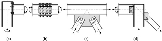
Figure 1.
Typical steel connections. The connection plates are shaded in grey: (a) Plate mainly in bending (plate is loaded in- and out-of-plane); (b–d) plates are loaded in-plane.
A possible way to categorize the connection plates was made in Table 1. The categorization is based on the loading situation (in-plane, out-of-plane) and the resulting behaviour of the plates (in- and out-of-plane deformations). Furthermore, the typical failure mechanisms and corresponding proofs (similar to EN 1993-1-8) are also given in Table 1.

Table 1.
Categorization of connection plates, depending on the loading situation and the deformation behaviour.
The focus of the presented research is on bolted plates (loads and deformations are in-plane). To check such plates, the designer had to choose a critical net section and had to calculate the corresponding stress components, depending on the geometry and the arrangement of the bolts. In doing so, the lower bound theorem and the Mises failure criterion are typically used.
The lower bound theorem, as well as the upper bound theorem, are theorems based on the plasticity theory. A detailed explanation, including proofs of the theorems, can be found, among others, in [3]. Especially, the lower bound theorem is typically chosen when designing steel connections in daily practice, which is also recommended by the Eurocode. Nevertheless, some checks in the EN 1993-1-8 are also based on the upper bound theorem, such as the T-stub model.
It should be mentioned that the theorems are only valid for ductile material behaviour, which can be assumed for the typically used mild steel grades (compare [4]). Furthermore, this is ruled in the EN 1993-1-10 [5] when designing steel constructions. Nevertheless, special attention is needed when the full plastic capacity cannot be reached, such as for local buckling problems (compare [6]) or bolts in tension. The cases considered here have drilled bolt holes, which means that stress concentrations will occur at the hole. The holes can be seen as mild notches, and the code rules a minimum distance between the holes. Therefore, it is assumed that the plates can reach their full plastic capacity. Pre-existing cracks, sharp notches, and other problems from fracture mechanics were typically not considered when designing such bolted connections, and is therefore, also not within the scope of this research.
As an alternative to the lower bound method in “hand calculations”, the engineer can also use numerical methods such as the finite element method (FEM). In this case, the geometrical behaviour is usually assumed as linear. The material behaviour can be modelled as linear-elastic or nonlinear. The linear-elastic calculation would often result in a conservative design, whereas the nonlinear simulation is much more realistic (especially when real stress-strain curves were considered [7]), but also computationally intensive (iterative solution methods are required). Furthermore, to calculate the whole connection realistically, even further aspects such as nonlinear contact formulations or appropriate strain criteria must be considered. Commercial software packages often do not provide such contact formulations, and strain criteria are usually not defined in codes, such as the maximum allowed strains for bearing failure (this will maybe change with the new Eurocode EN 1993-1-14, which is actually under progress).
The presented research focuses on an alternative method to overcome the problems mentioned above—the so-called discontinuity layout optimization (DLO). The DLO was first invented in [8,9] for plane plasticity problems, in analogy to truss layout optimization problems [10,11]. The first application was focused on geotechnical issues and the analysis of masonry arches [12]. Further research, especially on geotechnical problems, was made, among others, by [13,14,15]. Ongoing research was also focused on the extension to three-dimensional geotechnical issues [16,17]. A gradient-based adaptive solution method (ADLO) was presented in [18]. In addition to the plane plasticity problems, the DLO was also extended to analyze reinforced concrete slabs in [19,20,21]. For practical application of the before mentioned problems, the software LimitState [22] was invented.
The DLO procedure is based on the upper bound theorem, and therefore, results in an unsafe solution. If a load can be found, which also equals the solution from the lower bound theorem, then the correct loading capacity of the system was found (assuming an ideal-plastic material behaviour). The DLO procedure uses a broad set of possible failure mechanisms to overcome this problem. A linear programming (LP) algorithm tries to find the minimum load that the system collapses. Due to the discretization of the system with a limited number of failure mechanisms, the obtained load is still an upper bound but usually comes very close to the correct capacity [21,22].
The DLO procedure can be automatized for arbitrary geometries and loading situations, which is not the case for the lower bound method in “hand calculations”. The DLO procedure is much easier to use compared to the nonlinear FEM. Furthermore, no iterative solution methods are required because the nonlinear material behaviour (ideal-plastic) is implemented in the basic DLO formulation, which makes the technique a very efficient way to obtain the ultimate loads of arbitrary geometries and loading situations.
Research goal and strategy: Analyzing typical steel connections (as shown in Figure 1), but also more complex connections, is a “long term” goal. To reach this goal, the behaviour of the plates and the single components (as given in Table 1) must be analyzed systematically by the DLO approach. This also depends on the numerical implementation of the DLO method (mainly the degrees-of-freedom acting in-plane and out-of-plane). As a good starting point, the presented research focuses on the first row from Table 1. Analyzing plates loaded in-plane with a single bolt is the first step to check if the DLO procedure is suitable to handle such typical problems in steel connections. Furthermore, this research is the basis for further investigations on the other assemblies given in Table 1, but also on more complex connections.
Organization of the paper: First, the underlying concept of the DLO procedure was explained in detail and modified to handle slip line and yield zone mechanisms in Section 2. In contrast to geotechnical problems, the including of yield zones was necessary to reproduce the real behaviour of steel parts. For comparison, and also to get a better insight, the failure criteria from Tresca and Mises were both used in all simulations. The DLO procedure must be able to handle arbitrary geometries with and without holes for practical use in designing steel connections. As a first step, this was checked on basic cases in Section 3. Furthermore, the DLO procedure must be able to handle bolted connections too, which was investigated in Section 4 for plates with a single bolt. Therefore, a compression-only contact was implemented to reproduce the correct bearing behaviour. Case studies on steel parts with and without bolts were worked out with the DLO procedure and verified by solutions from the Eurocode EN 1993-1-8, literature, and from numerical simulations with the FEM, including parameter studies to figure out the influence of the discretization used.
2. Discontinuity Layout Optimization
The underlying concept of the DLO procedure is based on the upper bound theorem [9]. Instead of “hand calculations”, whereas a clearly defined collapse mechanism is chosen and analyzed, the DLO uses a large number of possible collapse mechanisms and searches for the mechanism with the lowest corresponding load. The collapse mechanisms are defined by dividing the geometry in a sufficient number of nodes. Each node is then connected to each other node by a discontinuity. A linear programming algorithm, including constraints, is used to find the collapse mechanism with the lowest resistance. The DLO concept is illustrated in Figure 2a–c, and the LP formulation can be seen from Equation (1).
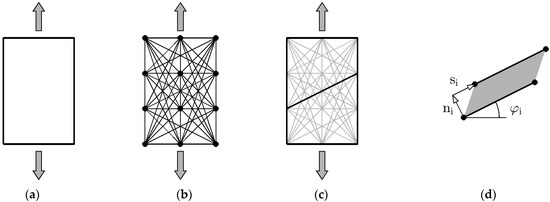
Figure 2.
Discontinuity layout optimization (DLO) procedure: (a) Geometry, loading, and boundary conditions; (b) discretization with nodes and discontinuities; (c) obtained collapse mechanism; (d) definition of a single discontinuity i.
The global vectors and are the unknowns in the LP formulation, whereas contains the relative shear and normal displacement jumps ( and ) of each local discontinuities (compare Figure 2d), and is a vector containing the corresponding local plastic multipliers . is a global compatibility matrix to ensure that at each node the sum of the shear and the normal displacement jumps equals zero (). The local compatibility matrix can be formulated with the direction cosines of each discontinuity i with:
is the global plastic flow matrix. Contrary to the formulation in [8], the local flow matrix and the local plastic multiplier allows shear and normal displacement jumps at each discontinuity:
In doing so, slip line mechanisms and yield zones are allowed to form at each discontinuity. By modifying , it is also possible to allow only slip lines or yield zones alone, which is shown in the further sections. Furthermore, the negative direction of the normal displacement jump of each discontinuity can be set to zero, which allows the implementation of a compression-only contact.
To formulate the (local) internal work of each discontinuity, the local vector is used. Corresponding to , the vector contains the shear strength , the yield strength , and the area ( and are the length and thickness, respectively) of discontinuity i:
The total internal work results in . The vector contains the external loads and the product represents the total external work done on the system, which is set to 1. In doing so, the output of the LP formulation is the dimensionless scalar , which can be interpreted as a failure load factor.
In the presented research, it was assumed that yielding at normal stresses always occur with . For the shear strength, two typical failure criteria for steel were used: The Tresca criterion with and the Mises criterion with . Typically, the Mises criterion is used in designing steel constructions. The DLO procedure results in an upper bound solution. Therefore, also the slightly more conservative Tresca criterion was considered.
The numerical implementation was done with the software MATLAB [23]. The DLO concept is used for scientific purposes only.
3. Case Studies on Tensile Specimens without Bolts
3.1. Tensile Specimen
As a first example, the tensile specimen from Figure 3a was considered. The specimen has the dimensions , , (plate thickness), and a steel grade S355 ().
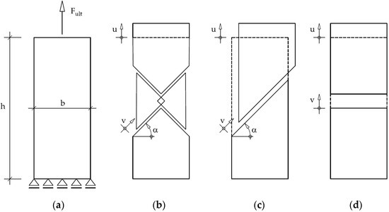
Figure 3.
Tensile specimen: (a) Loading and boundary conditions; (b) symmetrical slip line mechanism; (c) asymmetrical slip line mechanism; (d) yield zone mechanism.
First, the analytical solutions were obtained. A lower bound solution can be found by assuming a full plastic cross-section with:
An upper bound solution can be found by assuming the kinematic mechanism from Figure 3b, which consists of four identical slip lines. There is a small overlapping of the triangles in the middle of the plate, which means there is a small yield zone. For simplicity, the work of the yield zone is neglected, and the solution can be obtained by formulating the external and internal work equations:
The length of a single slip line can be expressed as . With , the work equation and the load function results in:
The minimum value of the load function can be found with . Depending on the used failure criterion (Tresca or Mises), the corresponding upper bound solutions result in:
The same load function can be obtained for the asymmetrical slip-line mechanism from Figure 3c. The only difference is the horizontal degree-of-freedom at the load introduction:
The kinematic mechanism (yield zone mechanism) shown in Figure 3d can be described similarly, and the upper bound solutions for the Tresca and the Mises criteria result both in the same value:
The same tensile specimen was analyzed with the DLO procedure. Figure 4a shows the automatic generated node distribution (software MATLAB [23]). The kinematic mechanisms (upper bound solutions), shown in Figure 4b–d, were obtained. The blue and red lines indicate a slip and a normal displacement behaviour, respectively.
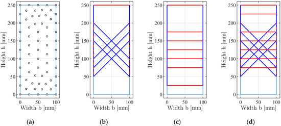
Figure 4.
Collapse mechanisms (blue: Slip displacements, red: Normal displacements) from DLO for the tensile specimen: (a) Nodes; (b) slip line mechanism; (c) yield zone mechanism; (d) combined slip line and yield zone mechanism.
The mechanism in Figure 4b was obtained for allowing slip line mechanisms only. The angle of the lines is precisely . Three identical mechanisms were obtained in comparison to Figure 3b. This occurred because each of the shown slip lines would result in the same minimum internal work. The linear programming algorithm divides the internal displacement equally to the indicated slip lines. Therefore, the higher the number of possible slip lines, the lower the internal work dissipated at each slip line. The total internal work is always the same, independent of the number of slip lines. Depending on the used failure-criterion, the corresponding loads result in and .
For comparison, if only yield zone mechanisms were allowed, the mechanism shown in Figure 4c was obtained. Again, the linear programming algorithm found more identical yield zones. The corresponding loads result in .
If slip line and yield zone mechanisms were both allowed in the DLO procedure, the Tresca criterion results in a combined mechanism, as shown in Figure 4d. In this case, all of the displayed slip lines and yield zones would dissipate the same internal work. The resulting load is always , independent of the number of slip lines and yield zones. For comparison, with the Mises criterion, the mechanism shown in Figure 4c was obtained. This happened because the yield zone mechanisms dissipate less internal work as the slip line mechanisms. Therefore, the linear programming algorithm divides the internal work equally only to the shown yield zones. Nevertheless, the load results also in .
The analytical number of possible mechanisms is ambiguous. It is well known from experiments that usually a single mechanism (a unique solution) forms, as shown in Figure 3b–d. Furthermore, this mechanism starts at a local defect or imperfection. These defects are not included in the “perfect” numerical model, which is the reason for the ambiguous solutions from the DLO procedure.
For comparison, numerical simulations with the FEM (software ANSYS [24]) were performed. A displacement driven nonlinear calculation with solid elements and a bilinear (linear-elastic, ideal-plastic) material behaviour was carried out. Mesh convergence studies were made to guarantee convergent solutions. The collapse mechanisms can be visualized by plotting the plastic strains after reaching the ultimate load (or the peak of the load-deflection curve [6]). Figure 5 shows the obtained mechanisms for a vertical displacement of . The ultimate loads resulted in and , depending on the used failure criterion.
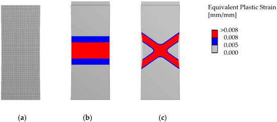
Figure 5.
Failure mechanisms (equivalent plastic strain) from a finite element analysis (FEA) for the tensile specimen: (a) Mesh; (b) yield surface according to the Tresca criterion was used; (c) yield surface according to the Mises criterion was used.
3.2. Tensile Specimen with a Hole
Figure 6a shows the same tensile specimen as used in Section 3.1, but now with a hole in the center of the specimen (diameter ).
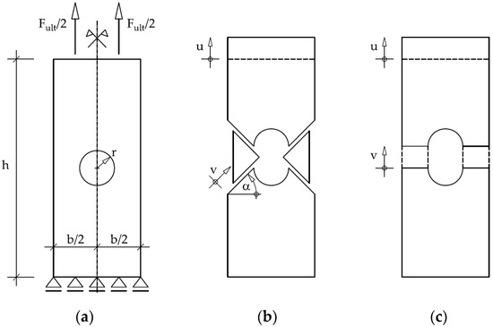
Figure 6.
Tensile specimen with a hole: (a) Loading and boundary conditions; (b) slip line mechanism; (c) yield zone mechanism.
A possible lower bound solution can easily be found by assuming a plastic net cross-section with
As mentioned in the introduction, the used constant plastic stress distribution is quite different from the elastic stress distribution, due to the stress concentration at the hole. The stress magnification depends mainly on the form and the size of the hole (such as for mild or sharp notches). In the presented research, only typical plates with holes from bolts (mild notches) and ductile material behaviour were considered, so the use of the lower bound theorem and the chosen constant plastic stress distribution are valid. The proof of the theorem and this example are also given in [3,25].
A possible upper bound slip line mechanism is shown in Figure 6b. The mechanism can be described similar to Equations (6) and (7):
Again, the minimum load can be obtained from the load function with . Using the same dimensions and failure criteria as in the previous section, the ultimate loads result in:
Another possible kinematic mechanism is the yield zone mechanism shown in Figure 6c. The mechanism can be described similar to Equation (10), with:
Only the left side of the symmetric system was used in the DLO procedure, to reduce the number of discontinuities. Figure 7a shows the automatic generated distribution of the nodes. If only slip line mechanisms were considered, the mechanism in Figure 7b was obtained with corresponding loads of and (for the whole system each). For the Tresca criterion, the load is 0.9% higher than the lower bound solution. The reason for this deviation is the inclination of the slip lines. The correct angle of cannot be reproduced exactly, with the used node distribution. With a more refined node distribution, the angle of the slip line tends to be (see Figure 7c,d) with an ultimate load of (still 0.4% higher). With a node distribution that includes slip lines with an angle of , the minimum load of can be found. An important fact is that this can also happen with a coarser node distribution. In general, the denser the node distribution, the higher the possibility to find a mechanism with lower resistance.
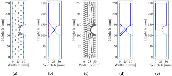
Figure 7.
Collapse mechanisms (blue: Slip displacements, red: Normal displacements) from DLO for the tensile specimen with a hole (only the left side of the symmetry model is shown): (a) Nodes; (b) slip line mechanism; (c) refined node distribution; (d) refined slip line mechanism, (e) yield zone mechanism.
The linear programming algorithm found the mechanism shown in Figure 7e for yield zone mechanisms only. The corresponding loads are .
By allowing slip line and yield zone mechanisms acting together, the LP-algorithm will find two identical solutions for the Tresca criterion (a slip line mechanism with and a yield zone mechanism, each with ). In this case, both mechanisms would be displayed (similar to Figure 4d). In the particular case (due to the node distribution with ), the load of the yield zone mechanism shown in Figure 7e is slightly lower than for the slip line mechanism. Therefore, only this mechanism was displayed. For the Mises criterion, the DLO always results in the mechanism from Figure 7e because the obtained load for the slip line mechanism is higher.
For comparison, this example was analyzed with the FEM. An ultimate load of was obtained with a yield-surface according to the Tresca criterion. Using the Mises criterion, the ultimate load results in . The small deviations to the lower bound solution results from numerical issues. The plastic mechanisms can be seen from Figure 8b,c for a vertical displacement of . Figure 8b shows a mixed mechanism (slip lines and yield zones). This corresponds to the results from the DLO approach (as explained, without discretization errors, the LP-algorithm will find two identical solutions for the Tresca criterion). The FEM is not based on an LP-algorithm, so the shown mixed mechanism was obtained directly.
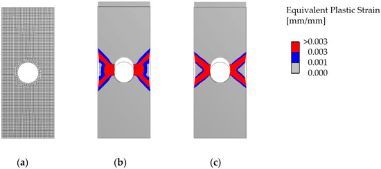
Figure 8.
Failure mechanisms (equivalent plastic strain) from a FEA for the tensile specimen with a hole: (a) Mesh; (b) yield surface according to the Tresca criterion was used; (c) yield surface according to the Mises criterion was used.
3.3. Tensile Specimen with Notches
As mentioned in the introduction, the focus of the presented research is mainly on bolted steel plates in connections. Nevertheless, also a tensile specimen with notches, as shown in Figure 9a, was also investigated to check the behaviour of the DLO approach. The failure mechanism depends on the size and shape of the notch. Therefore, similar to a bolted plate, only circular notches were considered (mild notch).

Figure 9.
Tensile specimen with notches: (a) Loading and boundary conditions; (b) slip line mechanism; (c) yield zone mechanism.
Figure 9a shows the same specimen as used in Section 3.2. Instead of the hole, two circular notches at the outside of the specimen with diameter were considered.
A possible lower bound solution is identical to Equation (11) and results in .
The slip line mechanism in Figure 9b was chosen similar to Figure 3b. For simplicity, the work of the small yield zone was neglected again. Furthermore, it was assumed that first yielding always starts at the point with the highest stress concentration, which is the notch in the particular case. After some calculus, the load function for the upper bound solution of this slip line mechanism can be found with:
and are the lengths of the lower and upper slip line, respectively. For the particular case, the lowest loads were calculated numerically by varying each angle from 0 to , and were found to be and . The corresponding angles are in both cases and .
The calculation of the yield zone mechanism in Figure 9c is identical to Equation (14) and the upper bound solution results in , which are 29% lower than the load from the slip line mechanism with the Tresca criterion. Furthermore, the load is identical to the load from the lower bound solution, which means that the ultimate load was found.
With the node distribution from Figure 10a, the DLO procedure for slip line mechanisms only, results in the mechanism shown in Figure 10b, with and . Using another node distribution, the mechanism in Figure 10c with and was obtained. The small deviation to the calculated load from Equation (15) comes from the slightly different inclinations of the slip lines ( and ), due to the node distribution.
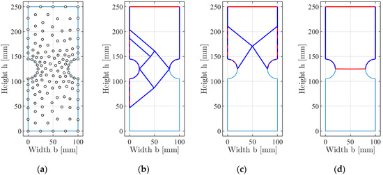
Figure 10.
Collapse mechanisms (blue: Slip displacements, red: Normal displacements) from DLO for the tensile specimen with notches: (a) Nodes; (b) asymmetrical slip line mechanism; (c) symmetrical slip line mechanism; (d) yield zone mechanism.
The obtained slip line mechanisms are similar to the assumed mechanism from Figure 9b. Furthermore, the loads are quite the same. It can be seen that the node distribution, and especially the inclinations of the discontinuities, have a significant influence on the mechanism, but the resulting loads are very similar. Nevertheless, the DLO approach found a (slightly) better failure mechanism than it was assumed first by hand calculation.
If yield zone mechanisms were allowed too, upper bound values of were obtained, see Figure 10d. This value equals the lower bound solution, and so the ultimate limit load was found. It can be seen that neglecting yield zone mechanisms would lead, in some cases, to mechanisms with much higher resistances.
Figure 11 shows the results from a finite element analysis (FEA) of the same example and a vertical displacement of . The Tresca criterion results in an ultimate load of and the Mises criterion in . A large yield zone between the notches was formed in both cases.
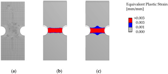
Figure 11.
Failure mechanisms (equivalent plastic strain) from a FEA for the tensile specimen with notches: (a) Mesh; (b) yield surface according to the Tresca criterion was used; (c) yield surface according to the Mises criterion was used.
If the results from the Mises criterion only were compared, it can be seen that the ultimate load from the FEA is larger than the ultimate load from the upper bound solution, which is contradictory. The reason is that the yield strength was considered with in the DLO procedure. Due to the real stress state, significant stresses normal to the load direction arise between the notches. Therefore, higher stresses (above ) in load direction are necessary that the material starts yielding. The maximum possible value, according to the Mises criterion, is . In the particular case, the critical stress that the material starts yielding can be recalculated by comparing the results from DLO and FEM. The critical stress corresponds to . This value was also reproduced by comparing the individual stress components from the FEA. In this particular case, the notches have a positive influence on the Mises criterion (and so on the ultimate load). From a practical point of view, if only the yield strength is assumed, the obtained resistance is conservative.
For comparison, the same tensile specimen was now investigated with a relative small distance between the notches (deep notches). Therefore, the distance between the notches was simply reduced to a neck width of 20 mm as shown in Figure 12.
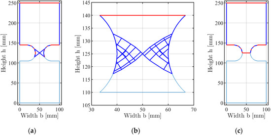
Figure 12.
Collapse mechanisms (blue: Slip displacements, red: Normal displacements) from DLO for the tensile specimen with deep notches: (a) Slip line mechanism; (b) sub-model with refined slip line mechanism; (c) yield zone mechanism.
A lower bound solution can easily be found by assuming a full plastic net section, which results in .
The upper bound solutions were calculated with the DLO approach. Assuming slip line mechanisms only, the mechanism in Figure 12a was obtained, which is quite different from the mechanisms in Figure 10b,c. Due to the coarse node distribution, a sub-model of the neck was created with a much finer node distribution. The refined slip line mechanism is shown in Figure 12b, with corresponding loads of and .
Allowing also yield zone mechanisms, the DLO approach results in the mechanism shown in Figure 12c. A refined analysis with a sub-model is not necessary for this case. The load results in , which equals the lower bound solution.
By concerning the examples from the previous sections, it can be drawn that slip line and yield zone mechanisms should be considered both in the DLO formulation. The so obtained loads correspond in all cases to the lower bound solution. Applying slip line or yield zone mechanisms only, leads sometimes not to the lowest resistance. Therefore, the following investigations were always carried out by including slip line and yield zone mechanisms acting together.
4. Case Studies on Tensile Specimens with a Single Bolt
4.1. Compression-Only Contact
It is necessary to have the possibility to consider a compression-only contact when modelling bolted connections. This can easily be implemented in the DLO procedure, by allowing only negative normal displacements at the relevant discontinuities by adopting Equation (3). The tension specimen from Figure 3a was used to test the contact behaviour. The only change is that the boundary condition at the bottom edge was set to a compression-only contact. Now, two scenarios were tested. In the first case, a tension force acts at the top edge (force direction upwards), and in the second case, a compression force acts at the top edge (force direction downwards).
For the tensile force, the pure translation mechanism shown in Figure 13b was obtained with an ultimate load of . This means that no internal work was dissipated (no collapse mechanism was formed) and a rigid body motion of the whole system occurred (translation upwards). For the compression force, the combined mechanism in Figure 13c was obtained for the Tresca criterion and the yield zone mechanism in Figure 13d for the Mises criterion. Both mechanisms result in the same ultimate load of . The implementation of the compression-only contact shows the correct behaviour.
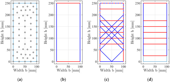
Figure 13.
Collapse mechanisms (blue: Slip displacements, red: Normal displacements) for a specimen with a compression-only support at the bottom edge and a tension or compression force at the upper edge: (a) Nodes; (b) tension force; (c) compression force and Tresca criterion; (d) compression force and Mises criterion.
It should be noted that for compression forces, the stability behaviour of the structure must be taken into account. This is not possible within the presented DLO formulation because additional degrees-of-freedom (out-of-plane) would be necessary to simulate such a buckling problem (compare Table 1). The focus of the particular case is to test the compression-only contact. Therefore, it was assumed that the specimen is restrained out-of-plane, and no buckling phenomena can occur.
In the following sections, the behaviour of a tensile specimen with a single bolt, as shown in Figure 14, was analyzed. According to EN 1993-1-8, the geometry can be described by the edge distances and . The bolt diameter and the diameter of the bolt hole are and , respectively. Real connections usually have a bolt-hole clearance, which must be considered in the simulation. This is not possible within the presented compression-only contact formulation. Therefore, the first investigations were performed for fit bolts (). A more realistic way, which covers the bolt-hole clearance, will be presented in Section 4.3 and Section 4.4.

Figure 14.
Plate in bearing with bolt and loading situation.
First, a convergence study to the number and distribution of the nodes and discontinuities for pure bearing failure was carried out. Therefore, relative large edge distances with were used. The discontinuities at the compression support between the bolt and plate dissipate no energy. This means that the first inner yield line next to the compression support will form a very local yield zone. Therefore, a denser nodal distribution next to the support is necessary. The nearer the first inner yield lines come to the support, the shorter the length of the involved yield lines and so the accomplished work. This behaviour can be seen in Figure 15.
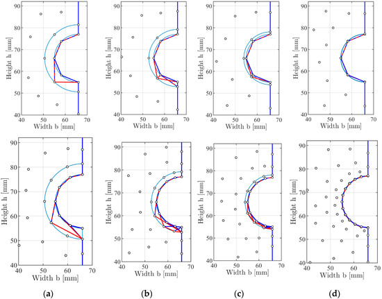
Figure 15.
Collapse mechanisms (blue: Slip displacements, red: Normal displacements) from DLO at the compression-only support for different node distributions (top row: Coarse mesh; bottom row: Fine mesh), the Mises criterion and different values: (a) ; (b) ; (c) ; (d) .
The nodes of the compression-only support lie on a circle with diameter . A second ring of nodes (and so of discontinuities) with diameter () was introduced to check the influence of the node distribution. A parameter study was carried out with different values for and different node distributions (see Figure 15). All calculations were carried out with the Tresca and the Mises criteria. The corresponding loads are given in Table 2. As expected, the lowest loads were obtained for decreasing values, and a converged solution can be found for . The influence of the node distribution (the number of nodes on the ring) is generally low and vanishes for . Furthermore, for lower values, a pure yield zone mechanism forms. In this case, there is no difference between the Tresca and the Mises criteria, which can be seen from Table 2.
Table 2.
Ultimate loads in kN for different values and different node distributions (first value: Tresca criterion; second value: Mises criterion; third value: Total number of nodes around the hole).
For comparison, if we assume a simple yield zone at the compression support, the corresponding load can be calculated with , which is in good accordance with the results from the DLO. This can be explained by looking at the discontinuities around the hole. The complete bearing resistance is the sum of the single resistances acting in force direction of each discontinuity, which equals the projected area used in the before mentioned formula. For the finest node distribution, a deviation of 62.55/62.48 = 1.0011 results, but for , only a small difference of approximately 1% (63.3/62.48 = 1.013) occurred. For , numerical problems arose in some cases. Therefore, is used for all further calculations.
4.2. Bearing Capacity for Smaller Edge Distances
The bearing capacity of a bolted plate depends strongly on the edge distances and . The four cases given in Table 3 were analyzed to study the behaviour of the DLO (case 1 concerns the investigations from Section 4.1). The chosen edge distances correspond to the relevant distances from EN 1993-1-8. According to the code, the value signals that the full bearing capacity can be reached and the value is the minimum allowed edge distance.
Table 3.
Overview, dimensions, and ultimate loads in kN for the considered cases.
Numerical simulations with the FEM were carried out. A mesh convergence study was performed for each calculation, so the following results are convergent solutions. The obtained failure mechanisms (equivalent plastic strains) can be seen from Figure 16. As expected, case 1 results in a pure bearing failure mechanism, while the other cases show “real” kinematic failure mechanisms. The corresponding ultimate loads are given in Table 3. Only the Mises criterion was used for the FE-simulations because it is well known that the Mises criterion predicts a better approximation to the real behaviour from experiments.
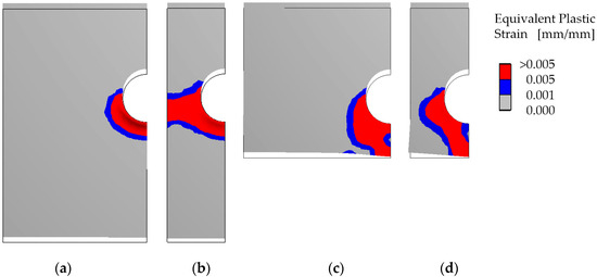
Figure 16.
Failure mechanisms (equivalent plastic strain, yield surface according to the Mises criterion) from a FEA for a displacement of 0.5 mm: (a) Case 1; (b) Case 2; (c) Case 3; (d) Case 4.
Now, the four cases were calculated with the DLO procedure. Both failure criteria were used because the DLO is still an upper bound method. A convergence study similar to the previous section has been worked out, so the given values are convergent solutions. The failure mechanisms can be seen from the top row of Figure 17. In all cases, independent of the failure criterion used, a pure bearing failure mechanism occurred. Furthermore, all cases result in the same bearing capacity of approximately , which means that the edge distances have no influence. The explanation of this obviously wrong behaviour can be seen from the FE-simulations. A three-dimensional stress state forms at the compression support. Such a stress state (and so the bearing behaviour) cannot be reproduced adequately with the DLO.
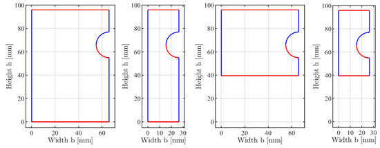
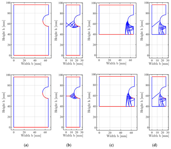
Figure 17.
Failure mechanisms (blue: Slip displacements, red: Normal displacements) from DLO (top row: Tresca and Mises criteria, ; middle row: Tresca criterion, ; bottom row: Mises criterion, ): (a) Case 1; (b) Case 2; (c) Case 3; (d) Case 4.
To overcome this problem, an approach was made by applying a higher yield strength only for yield zones in compression with (). In doing so, a value for the modification factor must be chosen, which was done by scaling the loads from the FEA and the DLO procedure with . Afterwards, the four cases were recalculated with the higher yield strength. The loads from the DLO procedure result in for case 1. The results of the other cases are summarized in Table 3, and the corresponding failure mechanisms are shown in Figure 17. The collapse mechanisms from the FEA and the DLO, independent of the failure criterion, show a good agreement. The collapse loads calculated with the Tresca criterion show a better correlation to the results from the FEA.
The presented approach with the modification factor seems to be a suitable calibration method, so the factor will be calibrated by more realistic bearing capacities from codes in the following section.
4.3. Bearing Capacity from Codes
The given bearing resistances in codes are usually higher than the bearing capacities from FE-simulations carried out with a bilinear material behaviour. Especially for large edge distances, very high bearing resistances can be obtained from experiments. Furthermore, the given formulas in codes are often based on the tensile strength (including the partial safety factor ) and not on the yield strength . The modification factor can be obtained by comparing the bearing resistance from the Eurocode EN 1993-1-8 with the DLO approach to consider the higher resistances. Within this approach, also the bolt-hole clearance can be considered now. Assuming a typical steel grade S355, the modification factor for the maximum bearing resistance results in:
According to the code, also the proof of the net cross-section under tension is necessary. This can be implemented in the DLO procedure with the same approach, which results in:
This means that no additional modification factor for tension forces is necessary for the DLO procedure. For comparison, also an approach from Moze [26] was used. This approach is less conservative than the Eurocode and independent from the edge distance , with:
With the given dimensions, the modification factor results in (including the bolt-hole tolerance, ). For comparison, also the ultimate loads for fit bolts () with were calculated. With these assumptions, the ultimate loads of the four cases from Section 4.2 were calculated and compared. The results are summarized in Table 4 and the failure mechanisms are shown in Figure 18.
Table 4.
Comparison of the ultimate loads in kN for the considered cases.

Figure 18.
Failure mechanisms (blue: Slip displacements, red: Normal displacements) from DLO with (top row: Tresca; bottom row: Mises): (a) Case 1; (b) Case 2; (c) Case 3; (d) Case 4.
With the DLO approach, now the bearing capacity for case 1 is significantly higher but still lower than the value from the code or literature. The reason can be seen from Figure 18a. The failure mechanism shows no longer a pure bearing mechanism. The resistance of the yield zone in compression is now much higher than the resistance of the obtained slip line mechanism. This means that it is not possible to reach the bearing capacity from the code with the DLO approach. The behaviour of the DLO procedure seems to be correct. In experiments usually, huge deformations occur, while the load is still increasing slowly. Therefore, the given resistances in codes are often based on a deformation criterion. Such load-deflection curves can be found in the literature (see, among others [26,27,28]). The mechanisms and the resistances of the other three cases are similar to the mechanisms from Figure 17.
The ultimate loads calculated with and are quite the same, which means that the influence of the bolt-hole tolerances can be neglected. This was checked by further calculation with , which results still in the same loads. Therefore, a value of was used for all coming simulations.
4.4. Parameter Study
A parameter study has been worked out to get a better insight into the behaviour of the DLO procedure concerning different edge distances. The parameter range was chosen with and . A steel grade S355 was used. The bearing resistance and the proof of the net section must both be checked. These proofs are automatically included in the resistances from the DLO procedure. For an objective comparison, the resistances from the code EN 1993-1-8, from literature (Equations (18) and (19)), and also the ultimate loads from the DLO procedure were normalized, as shown in Figure 19.
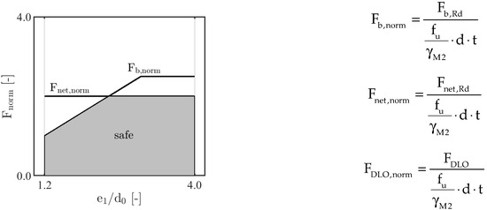
Figure 19.
Normalization of the loads from codes, literature, and DLO.
The normalized forces depend still on the ratio of bolt-hole diameter and bolt. Therefore, two representative cases have been worked out. The first case considers a value of , which represents a typical bolt-hole tolerance, e.g., M20 bolts. For comparison, the second case considers no bolt-hole tolerance with . The geometry in the DLO procedure was always modelled with . The calculated and normalized loads are shown in Figure 20 and Figure 21.
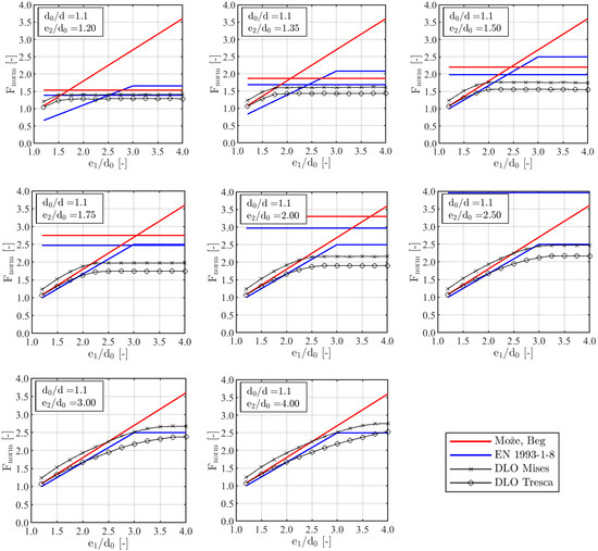
Figure 20.
Comparison of normalized loads for .
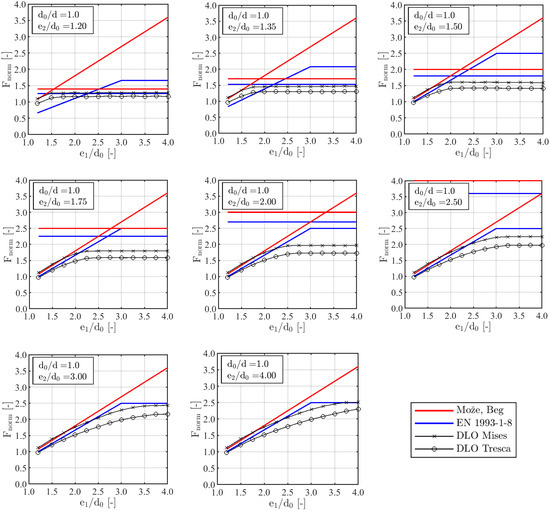
Figure 21.
Comparison of normalized loads for .
The loads according to Equations (18) and (19) are significantly higher than the loads from EN 1993-1-8. Especially for small edge distances with and , but also for large edge distances with and . In [26], it is explained that the value in Equation (16) was only included due to lack of experimental evidence and that for small edge distances the values in EN 1993-1-8 are very conservative. Furthermore, for larger edge distances the question for the need of an upper limit (actually ) arose. It was stated that if no limit is defined, then the shear resistance of the bolt is automatically an upper limit. Still, if a limit should be set, then a bearing stress of would be an appropriate value for the ultimate resistance. Further information was given to prevent a too large hole elongation for service loads, but this is not part of the presented research.
A similar behaviour was obtained for and . As expected, the DLO procedure with the Mises criterion delivers in all cases higher loads than the Tresca criterion. Especially for combined with smaller edge distances and , the loads obtained with the Mises criterion are slightly unsafe compared to Equations (18) and (19). For larger edge distances and , the DLO resistances are (in some cases significant) lower than the resistances from Equations (18) and (19). The loads from the DLO procedure are similar to the loads from EN 1993-1-8 for very large edge distances. This happened because an upper limit with 2.5 is considered in the code. As explained in Section 4.3, the full bearing resistance can only be reached, if there is no other failure mechanism with a lower resistance, e.g., as shown in Figure 18.
5. Discussion and Conclusions
A modified DLO procedure for steel parts without bolts and steel connections with a single bolt was presented. The modified approach includes slip line and yield zone mechanisms acting together. Furthermore, a compression-only contact was included too. A modification factor for single bolts has been worked out to ensure the correct bearing behaviour. For all considered cases, a comparison between the ultimate loads from DLO, literature, and Eurocode EN 1993-1-8 were made. The following conclusions can be drawn:
First, specimens without bolts were investigated. It was shown that slip line and yield zone mechanisms must both be included, otherwise mechanisms with higher loads were obtained in some cases. In doing so, the DLO procedure shows in all cases a correct behaviour. The LP-algorithm was able to find in all considered cases the minimum load, which corresponds to the lower bound solution, and therefore, equals the correct ultimate load, independent of the failure criterion used.
For bolted specimens, the simple case of a connection with a single bolt was considered. It was found that a second ring of discontinuities close to the bolt hole is necessary to obtain convergent solutions, represented by the modification factor . Compared to the bearing resistances from codes, the DLO delivers conservative loads in many cases. Therefore, the modification factor was recalculated from the Eurocode and literature, and verified by a parameter study. Depending on the edge distances, the DLO results still in conservative resistances for most of the cases.
A first study to the application of the DLO procedure to steel parts and steel connections has been presented in this paper. In general, the behaviour and the obtained loads are in a good agreement with the analytical solutions and the results from the FEA. Therefore, future work will be done in this field of research, which will focus on more sophisticated connections with bolt groups and further components (as stated in Table 1). Compared to standards, the DLO can also be used to analyze “automatic” arbitrary geometries (such as the FEM). Compared to the FEM, the DLO approach is much simpler for calculating the limit load. Maybe one day, the DLO could also become a standard tool in designing steel constructions and connections as the FEM already is.
Funding
The open access fee was funded by the publication fund of the University of Innsbruck.
Acknowledgments
The author would like to thank the University of Innsbruck, for giving me the opportunity to carry out this research and for providing the open access funding.
Conflicts of Interest
The author declares that there is no conflict of interest. The funder had no role in the design of the study, in the collection, analyses, or interpretation of data, in the writing of the manuscript or in the decision to publish the results.
References
- EN 1993-1-8. Eurocode 3: Design of Steel Structures, Part 1-8: Design of Joints; CEN European Committee for Standardization: Brussels, Belgium, 2012. [Google Scholar]
- Jaspart, J.-P.; Weynand, K. Design of Joints in Steel and Composite Structures; ECCS—European Convention for Constructional Steelwork and Ernst & Sohn: Berlin, Germany, 2016; ISBN 978-92-9147-132-4. [Google Scholar]
- Kaliszky, S. Plastizitätslehre: Theorie und technische Anwendungen; Akadémiai Kiadó: Budapest, Hungary, 1984; ISBN 963-05-3196-8. [Google Scholar]
- Feldmann, M.; Schäfer, D.; Eichler, B. Vorhersage duktilen Festigkeitsversagens von Stahlbauteilen mit Hilfe schädigungsmechanischer Methoden. Stahlbau 2009, 78, 784–794. [Google Scholar] [CrossRef]
- EN 1993-1-10. Eurocode 3: Design of Steel Structures, Part 1-10: Material Toughness and Through-Thickness Properties; CEN European Committee for Standardization: Brussels, Belgium, 2005. [Google Scholar]
- Timmers, R.; Lener, G. Collapse mechanisms and load–deflection curves of unstiffened and stiffened plated structures from bridge design. Thin-Walled Struct. 2016, 106, 448–458. [Google Scholar] [CrossRef]
- Yun, X.; Gardner, L. Stress-strain curves for hot-rolled steels. J. Constr. Steel Res. 2017, 133, 36–46. [Google Scholar] [CrossRef]
- Smith, C.; Gilbert, M. Application of discontinuity layout optimization to plane plasticity problems. Proc. R. Soc. A Math. Phys. Eng. Sci. 2007, 463, 2461–2484. [Google Scholar] [CrossRef]
- Smith, C.; Gilbert, M. Evaluating Displacements at Discontinuities within a Body. UK Patent GB2442496A, 9 April 2008. [Google Scholar]
- Gilbert, M.; Tyas, A. Layout optimization of large-scale pin-jointed frames. Eng. Comput. 2003, 20, 1044–1064. [Google Scholar] [CrossRef]
- He, L.; Gilbert, M.; Song, X. A Python script for adaptive layout optimization of trusses. Struct. Multidiscip. Optim. 2019, 60, 835–847. [Google Scholar] [CrossRef]
- Gilbert, M.; Smith, C.; Pritchard, T.J. Masonry arch analysis using discontinuity layout optimisation. Proc. Inst. Civ. Eng. Eng. Comput. Mech. 2010, 163, 155–166. [Google Scholar] [CrossRef]
- Smith, C.; Gilbert, M.; He, L.; González-Castejón, J.; Ouakka, S. Recent advances in the application of discontinuity layout optimization to geotechnical analysis and design problems. In Proceedings of the XVII ECSMGE-2019; The Icelandic Geotechnical Society: Reykjavik, Iceland, 2019; ISBN 978-9935-9436-1-3. [Google Scholar]
- Smith, C.; González-Castejón, J.; Charles, J. Enhanced interpretation of geotechnical limit analysis solutions using Discontinuity Layout Optimization. In Proceedings of the 19th International Conference on Soil Mechanics and Geotechnical Engineering, Seoul, Korea, 17–22 September 2017; pp. 851–854. [Google Scholar]
- Zhang, Y.; Zhuang, X.; Lackner, R. Stability analysis of shotcrete supported crown of NATM tunnels with discontinuity layout optimization. Int. J. Numer. Anal. Methods Géoméch. 2018, 42, 1199–1216. [Google Scholar] [CrossRef]
- Zhang, Y. Multi-slicing strategy for the three-dimensional discontinuity layout optimization (3D DLO). Int. J. Numer. Anal. Methods Géoméch. 2016, 41, 488–507. [Google Scholar] [CrossRef] [PubMed]
- Hawksbee, S. 3D Ultimate Limit State Analysis Using Discontinuity Layout Optimization. Ph.D. Thesis, University of Sheffield, Department of Civil and Structural Engineering, Sheffield, UK, 2012. [Google Scholar]
- Bauer, S.; Lackner, R. Gradient-based adaptive discontinuity layout optimization for the prediction of strength properties in matrix–inclusion materials. Int. J. Solids Struct. 2015, 63, 82–98. [Google Scholar] [CrossRef]
- Gilbert, M.; He, L.; Smith, C.; Le, C. Automatic yield-line analysis of slabs using discontinuity layout optimization. Proc. R. Soc. A Math. Phys. Eng. Sci. 2014, 470, 20140071. [Google Scholar] [CrossRef] [PubMed]
- He, L.; Gilbert, M. Automatic rationalization of yield-line patterns identified using discontinuity layout optimization. Int. J. Solids Struct. 2016, 84, 27–39. [Google Scholar] [CrossRef]
- He, L.; Gilbert, M.; Shepherd, M. Automatic Yield-Line Analysis of Practical Slab Configurations via Discontinuity Layout Optimization. J. Struct. Eng. 2017, 143, 04017036. [Google Scholar] [CrossRef]
- LimitState: Analysis & Design Software for Engineers; LimitState Ltd.: Sheffield, UK. Available online: http://limitstate.com (accessed on 5 April 2020).
- Matlab: Version: R2018a, Software; The MathWorks, Inc.: Natick, MA, USA. Available online: https://de.mathworks.com (accessed on 27 April 2020).
- Ansys: Version: 2019 R1, Engineering Simulation & 3D Design Software; ANSYS, Inc.: Canonsburg, PA, USA. Available online: www.ansys.com (accessed on 12 February 2020).
- Mang, H.; Hofstetter, G. Festigkeitslehre, 4th ed.; Springer Vieweg: Berlin/Heidelberg, Germany, 2013. [Google Scholar]
- Može, P.; Beg, D. A complete study of bearing stress in single bolt connections. J. Constr. Steel Res. 2014, 95, 126–140. [Google Scholar] [CrossRef]
- Draganić, H.; Dokšanović, T.; Markulak, D. Investigation of bearing failure in steel single bolt lap connections. J. Constr. Steel Res. 2014, 98, 59–72. [Google Scholar] [CrossRef]
- Može, P.; Beg, D. Investigation of high strength steel connections with several bolts in double shear. J. Constr. Steel Res. 2011, 67, 333–347. [Google Scholar] [CrossRef]
© 2020 by the author. Licensee MDPI, Basel, Switzerland. This article is an open access article distributed under the terms and conditions of the Creative Commons Attribution (CC BY) license (http://creativecommons.org/licenses/by/4.0/).