Effective Suppression of Residual Magnetic Interference in a Conductive Shielded Room for Ultra-Low Field Nuclear Magnetic Resonance

Abstract

Residual magnetic interference induced by applied magnetic field pulses inside a conductive shielded room (SR) has been a common issue in ultra-low-field (ULF) nuclear magnetic resonance (NMR). The rapid cutoff of the applied pre-polarizing field (B_p) induces eddy currents in the walls of the SR, which produces a decaying residual magnetic interference that may cause severe image distortions and signal loss. In this study, a pair of cancellation coils (CC) and control electronics were designed for the suppression of the residual magnetic interference in a SR. Simulations show that this method was effective in suppressing the residual magnetic field (B_r) after removal of the pre-polarizing magnetic field. Then, a small-scale SR was designed and the effectiveness of this cancellation scheme was experimentally verified. The test results showed a good agreement with the simulation, which indicated that the cancellation scheme was capable of reducing B_r field to a much lower level. The scheme proposed in this study provides a solution for suppressing the residual magnetic field in the ULF NMR system. After decoupling the eddy–current field, the effect of the suppression may be further improved by optimization of the cancellation coil in further work.

1. Introduction

Ultra-low-field nuclear magnetic resonance (ULF NMR) is one of the hot research areas in the applications of superconducting quantum interference device (SQUID) [1,2,3]. Compared with the measurement field (B_m) strength in the conventional high-field apparatuses (HF-MRs) [4], the measurement field strength in ULF NMR is several orders of magnitude lower, which brings some advantages including inhomogeneous line broadening comparable to natural line widths or narrower, absence of distortion artifact with metal and chemical shift due to the strong main field and ease of B_m tuning over many octaves. As well as lower cost and decrease in volume, it is possible to obtain unique images with enhanced longitudinal relaxation time contrast [5]. The significantly lower measurement magnetic field in comparison with 1.5 T hospital MRI or 9 T lab MRI causes the reduction of signal-to-noise ratio, thus normally ULF NMR introduces strong pre-polarizing field (B_p) and works in magnetically shielded environments [6]. A pulsed B_p whose amplitude is 2–3 orders-of-magnitude stronger is critical to SNR enhancement since the signal amplitude is proportional to B_p strength [7,8,9,10]. However, pulsed operation of the B_p coil may magnetize and induce large eddy currents around shielding structures such as a magnetically or conductive shielded room. The transient magnetic field generated by the eddy currents may cause severe image distortions and signal loss, especially when the large pre-polarizing coil are employed for in vivo imaging [7].

A method for the assessment of magnetic properties of ferromagnetic materials at low magnetic field values was presented by Canova, A. et al. [11] and they designed a magnetically shielded room which can be effective against low-frequency external magnetic field disturbances. Li B. et al. [12] calculated and simulated the shielding effectiveness of the shielded room with different thicknesses of aluminum sheets to increase the SNR and improve image quality. Dong H. et al. [13] according to the relative position of the B_p coil and the shielded room, described two physical models of the conductive shielded room to simulate the transient fields at the sample position: the B_p coil plane parallel to the ceiling and floor of the shielded room and the coil plane perpendicular to the walls. In [14], superconducting connectivity technique was utilized to connect input coil and pickup coil in order to obtain the best SNR of the fetal magnetocardiography signals in a thin magnetically shielded room.

Suppression of the residual magnetic field (B_r) makes it possible to increase the upper value of B_p and the magnetization intensity of the object to be measured. In [15], an effective method to design self-shielded polarizing coils for ULF NMR by connecting shielding coils and the polarizing coil in series with reversed currents was presented and the magnetic fields caused by the eddy currents were largely reduced. In their works the residual magnetic field enters steady state at about 300 ms while in our works the residual magnetic field enters steady state at about 110 ms. In [16], cancellation coils (CC) with discrete current loops connected in serial to the B_p coil was implemented using the method of inverse problem and it effectively neutralizes the magnetic field produced by the B_p coil on the SR walls. Zevenhoven, K. C. J et al. [17] introduced a dynamical cancellation method in which a precisely designed current waveform was applied to a separate coil after turning off the polarizing pulse. Complicated calculation is needed to figure out the cancellation current density distribution in [16] or the precisely designed cancellation current waveform in [17], while it was avoided in this study. By changing the number of turns of the CC which is connected in series with the B_p coil in the designed structure in this study, the residual magnetic field was suppressed effectively.

In this study, to reduce the impact of B_r field inside a SR, a simple method which includes a pair of CCs symmetrically distributed along the B_p coil and a control electronics which can generate appropriate current for the B_p coil and the CC is presented. Simulation and experiment both show that this method can effectively suppress the residual magnetic interference in a small-scale SR. Simulation shows that with 70 turns CC, B_r decays much faster than without CC and enters stable state very early once the B_p current switched off.

2. Theory

In previous research, it was found that the eddy currents in the SR can be modeled as a superposition of spatial patterns with amplitudes given by the elements of a vector $j(t)$, we can describe their excitation and dynamics by linear differential equations [18,19]

$$M\frac{\mathrm{d}j(t)}{\mathrm{d}t}+Rj(t)+m\frac{\mathrm{d}I(t)}{\mathrm{d}t}=0,$$

(1)

The elements on the diagonal of the symmetric matrix $M$ are the self-inductances of the spatial eddy–current patterns and off-diagonal terms are mutual inductances of the spatial eddy–current patterns. The matrix $R$ contains the resistances of the current patterns on its diagonal and the off-diagonal “mutual resistances” describe the Ohmic coupling between patterns that share the same conductor. The third term is an electromotive force (EMF) induced by the current I(t) in a coil, which couples to the eddy–current patterns via mutual inductance in the vector $m$.

The connection between magnetic field and eddy current can be expressed as

$$B(t)={\beta }^{T}j(t).$$

(2)

Here, $\beta$ is a coupling vector in which elements are corresponding to the points and magnetic-field components of interests [20] (the superscript T denotes the transpose).

Residual magnetic interference of pulse-induced transients has a significant influence on the magnetic signal to be measured and the residual magnetic is much smaller than the source magnetic that excites it. To observe it precisely, the residual magnetic shall be measured after the current through the B_p coil is completely switched off, because at that time it will dominate the magnetic field in the SR.

The current in B_p coil can be expressed as

$$\{\begin{array}{c}I(t)=k(1-\theta (t))\\ \frac{\mathrm{d}I(t)}{\mathrm{d}t}=-k\frac{\mathrm{d}\theta (t)}{\mathrm{d}t}=-k\delta (t)\end{array}.$$

(3)

Here, $\theta (t)$ is a unit step function, $\delta (t)$ is the unit pulse function, $k$ is the maximum value of current in B_p coil. Substituting $\frac{\mathrm{d}I(t)}{\mathrm{d}t}=-k\delta (t)$ into (1) and applying the Fourier transform, one can get $\mathrm{i}\omega M\widehat{j}(\omega )+R\widehat{j}(\omega )-km=0$, then

$$\widehat{j}(\omega )=k{(\mathrm{i}\omega M+R)}^{-1}m=k{\widehat{j}}_{ISR}(\omega )$$

(4)

in which ${\widehat{j}}_{ISR}(\omega )={(\mathrm{i}\omega M+R)}^{-1}m$. The ISR means the inverse-step response.

By applying Fourier transform to (1), we may obtain $\mathrm{i}\omega M\widehat{j}(\omega )+R\widehat{j}(\omega )+\mathrm{i}\omega m\widehat{I}(\omega )=0$. Hence

$$\widehat{j}(\omega )=-{(\mathrm{i}\omega {\rm M}+R)}^{-1}m\cdot \mathrm{i}\omega \widehat{I}=-{\widehat{j}}_{ISR}(\omega )\cdot \mathrm{i}\omega \widehat{I}(\omega ).$$

(5)

The inverse Fourier transform is performed to Equation (5) to get ($\ast$ denotes convolution)

$$j(t)=-(j_{ISR}\ast \frac{\mathrm{d}I}{\mathrm{d}t})(t).$$

(6)

Provided that the magnetic-field response to an inverse step current in Equation (3) is known, the time evolution of the eddy–current magnetic field transient B(t) caused by any pulse waveform I(t) can be computed by

$$B(t)=-(B_{ISR}\ast \frac{\mathrm{d}I}{\mathrm{d}t})(t).$$

(7)

Equation (7) is suitable to estimate transient magnetic field for the CC and B_p coil in the SR.

The currents in the B_p coil and CC are I_p(t) and I_c(t), respectively. Suppose the coil have individual inductances $m_p$ and $m_c$ with the eddy–current patterns, leading to corresponding magnetic fields, $B_{ISR}^{(p)}$ and $B_{ISR}^{(c)}$. The third term in Equation (1) becomes $m_p\frac{d{I}_p(t)}{dt}+m_c\frac{d{I}_c(t)}{dt}$ and the total transient magnetic field B(t) becomes

$$B(t)=-[(B_{ISR}^{(p)}\ast \frac{\mathrm{d}{I}_p}{\mathrm{d}t})(t)+(B_{ISR}^{(c)}\ast \frac{\mathrm{d}{I}_c}{\mathrm{d}t})(t).$$

(8)

In this study, the B_p coil is connected in series with the cancellation coil and they are both completely switched off in 2 ms. We take this moment as t_s = 2 ms. When t > t_s, $\frac{dI(t)}{dt}=0$ in Equation (1). Equation (1) can be written as

$$M\frac{dj(t)}{dt}+Rj(t)=0.$$

(9)

Then

$$\frac{dj(t)}{dt}=-{(M^{T}M)}^{-1}{M}^{T}Rj(t).$$

(10)

Finally, we can get

$$j(t)=e^{-{(M^{T}M)}^{-1}-M^{T}Rt}+K,$$

(11)

where K is a constant. K equals zero because in practice the eddy current in a SR will decay to zero. Combined with Equation (2), we can get

$$\begin{array}{cc}{B}_r(t)& ={\beta }^{T}j(t)\\ & ={\beta }^T{e}^{-{(M^{T}M)}^{-1}-M^{T}Rt}.\end{array}$$

(12)

Once the currents through B_p coil and CC completely switched off, we write B_r(t) as B(t).

Then combining Equations (8) and (12), gives

$$-[(B_{ISR}^{(p)}\ast \frac{\mathrm{d}{I}_p}{\mathrm{d}t})(t)+(B_{ISR}^{(c)}\ast \frac{\mathrm{d}{I}_c}{\mathrm{d}t})(t)={\beta }^T{e}^{-{(M^{T}M)}^{-1}-M^{T}Rt}$$

(13)

Based on Equation (13), it can be shown that the residual eddy–current magnetic field can be divided into two parts. The first part is produced by B_P coil and the second part by CC. According to reference [20], the residual eddy–current magnetic field can be expressed by

$$B_r(t)={\displaystyle \sum _{i=1}^N{A}_i}{e}^{-t/{\tau }_i}+C.$$

(14)

Combining Equations (13) and (14), when t > t_s = 2 ms

$$B_{r1}(t)=-(B_{ISR}^{(p)}\ast \frac{\mathrm{d}{I}_p}{\mathrm{d}t})(t)={\displaystyle \sum _{i=1}^{N_1}{A}_i}{e}^{-t/{\tau }_i}+C_1,$$

(15)

$$B_{r2}(t)=-(B_{ISR}^{(c)}\ast \frac{\mathrm{d}{I}_c}{\mathrm{d}t})(t)={\displaystyle \sum _{j=1}^{N_2}{A}_j}{e}^{-t/{\tau }_j}+C_2.$$

(16)

Here, N₁ and N₂ are positive integers; $A_i$, ${\tau }_i$ and ${\tau }_j$ are positive numbers; $A_j$ is a negative number; B_r1(t) and B_r2(t) represent the eddy–current magnetic field generated by B_P coil and CC coil in the SR, respectively and they are mutually offset.

3. Simulation

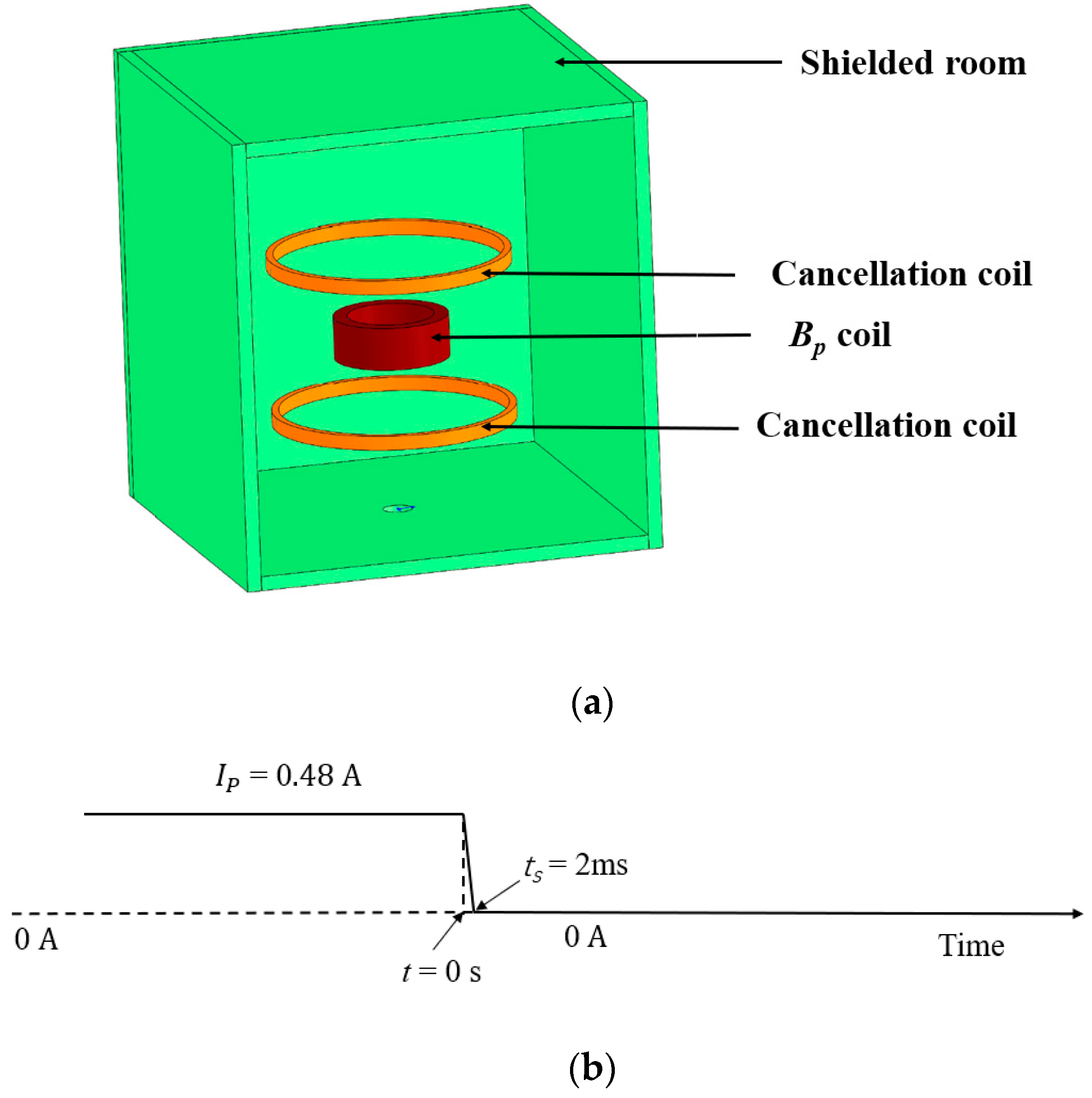
As a demonstration, a small-scale copper conductive SR was designed with dimension of 280 mm × 280 mm × 300 mm, and the wall thickness was 10 mm, as shown in Figure 1a. A pair of CCs was symmetrically configured above and below the B_p coil whose distance to each CC was 46 mm and the distance from B_p coil to the center of floor was 110 mm in the SR. The pair of CCs were connected in series with the B_p coil, so the current in the B_p coil was the same as that in the CC, but with opposite directions. The current was switched off in 2 ms. The parameters of the B_p coil and CC were shown in

Table 1. Parameters of the B_p coil and the cancellation coil.

Parameters	Bp coil	Cancellation coil (CC)
Material	Copper	Copper
Inside diameter	60 mm	160 mm
Outside diameter	80 mm	170 mm
Section area	300 mm2	50 mm2
Number of conductors	750	70

. The current through the B_p coil during the simulation is shown in Figure 1b.

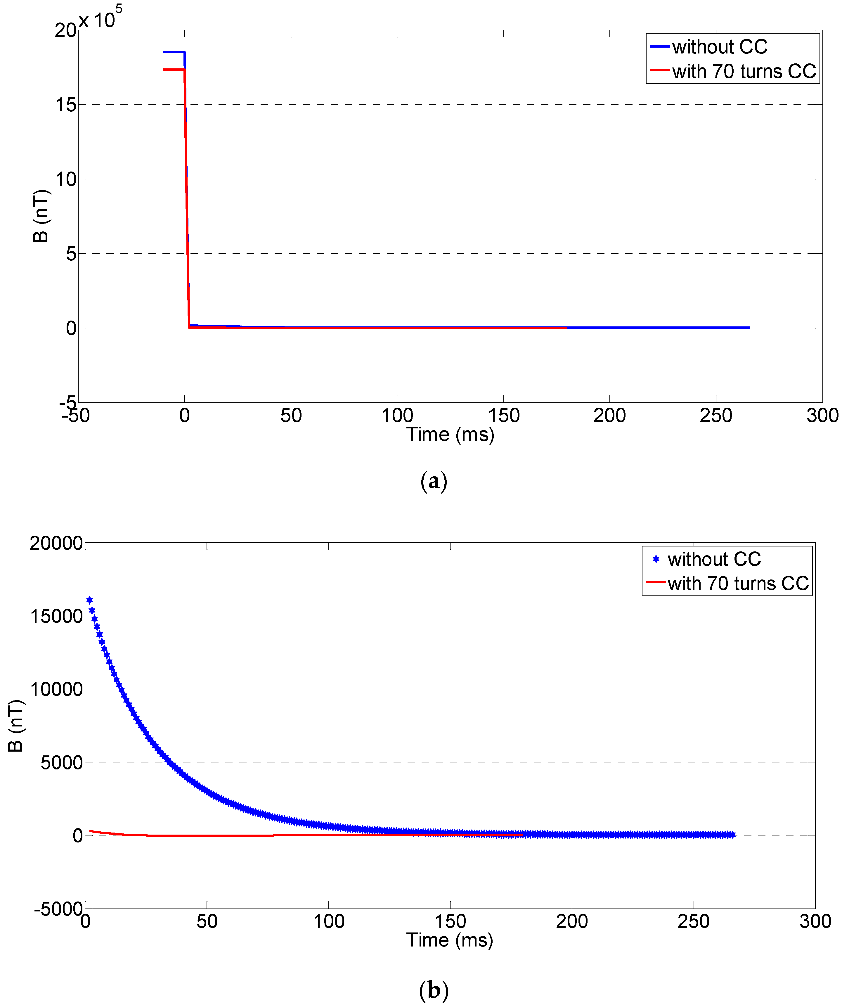
Figure 2 shows the comparison of residual magnetic field component in z direction without and with CC measured with the magnetic sensor HMC2003. It can be seen from Figure 2 and

Table 2. B_r without CC and with 70 turns CC at different times.

Br 1	0 ms	2 ms	10 ms	50 ms	100 ms
Without CC	1.85 × 106 nT	16,040 nT	11,850 nT	816 nT	848.1 nT
With 70 turns CC	1.73 × 106 nT	289.7 nT	103 nT	−59.51 nT	−24.57 nT

¹B_r is the residual magnetic field in z direction at the measuring point. TMmeasuring point is at the center of the top of B_p coil.

, B_r decayed much faster with the 70 turns CC configuration (In this configuration, the number of turns of CC was 70) than with no CC. When t > 10 ms, the B_r with 70 turns CC had already entered a very low stage and most of the attenuation occurs before 10 ms.

The number of turns of CC had a significant impact on the effect of the cancellation. Figure 3 shows the residual magnetic field at the measuring point when the number of turns of the CC changed from 64 to 78. Figure 3a shows that the suppression effects of the residual magnetic field were quite obvious and Figure 3b shows the comparison of the suppression effects with different number of turns of CC.

From Figure 3, it can be seen that the best result occurs when the CC has 70 turns. However, overshoot of the cancellation of the eddy–current magnetic field can be observed under this condition, partly because the dimensions of the cancellation coil have not been optimized well enough, which will be an important aspect to be studied in the future.

It can be seen from the analysis in Section 2 that the acquired measurements B_r(t) can be treated as a linear combination of exponentially decaying signals with multiple distinct time constants.

$$\{\begin{array}{c}{B}_r(t)=B_{r1}(t)+B_{r2}(t)\\ B_{r1}(t)=-(B_{ISR}^{(p)}\ast \frac{\mathrm{d}{I}_p}{\mathrm{d}t})(t)={\displaystyle \sum _{i=1}^{N_1}{A}_i}{e}^{-t/{\tau }_i}+C_1\\ B_{r2}(t)=-(B_{ISR}^{(c)}\ast \frac{\mathrm{d}{I}_c}{\mathrm{d}t})(t)={\displaystyle \sum _{j=1}^{N_2}{A}_j}{e}^{-t/{\tau }_i}+C_2\end{array}.$$

(17)

According to [20], we set $N_1=2$, $N_2=2$, $C_1=C_2=0$. $A_i$, ${\tau }_i$ and ${\tau }_j$ are positive numbers and $A_j$ is negative.

The expression of fitting curve B_z-fix1 in Figure 4 is

$$B_{z-fix1}=8535*e^{(-28.2t)}+8553*e^{(-45.2t)}.$$

(18)

Because there is no CC in this configuration and only the residual magnetic field in z direction is considered, eddy–current magnetic field is generated only by B_p coil in simulation.

Hence,

$$\begin{array}{cc}{B}_r& =B_{r1}=B_{z-fix1}\\ & =8535*e^{(-28.2t)}+8553*e^{(-45.2t)}.\end{array}$$

(19)

B_r1 represents the eddy–current magnetic field generated by the B_p coil.

The expression of fitting curve B_z-fix2 in Figure 5 is

$$B_{z-fix2}=8535*e^{(-28.2t)}+8553*e^{(-45.2t)}-8380*e^{(-42.96t)}-8372*e^{(-28.08t)}$$

(20)

Because there is CC in this configuration and only the residual magnetic field in z direction is considered, eddy–current magnetic field is generated by B_p coil and CC in simulation.

Hence,

$$\begin{array}{cc}{B}_r& =B_{r1}+B_{r2}=B_{z-fix2}\\ & =8535*e^{(-28.2t)}+8553*e^{(-45.2t)}-8380*e^{(-42.96t)}-8372*e^{(-28.08t)}.\end{array}$$

(21)

Combining Equations (19) and (21), we can get the expression of the eddy–current magnetic field generated only by CC,

$$B_{r2}=-8380*e^{(-42.96t)}-8372*e^{(-28.08t)}.$$

(22)

Therefore, we decouple the eddy–current magnetic field produced by the B_p coil and the CC in SR in simulation after the current is completely switched off at t_s = 2 ms into two parts:

$$\{\begin{array}{l}{B}_{r1}=8535*e^{(-28.2t)}+8553*e^{(-45.2t)}\\ B_{r2}=-8380*e^{(-42.96t)}-8372*e^{(-28.08t)}\end{array}$$

(23)

To date, we have simulated the suppression effect of the SR with CC on the eddy–current magnetic field and decoupled the eddy–current magnetic field produced by the B_p coil and the CC by data fitting. We will now experimentally verify these theoretical predictions.

4. Experimental Results

An equipment representative of the configuration previously studied was manufactured, as illustrated in Figure 6, with a plastic holder supporting coil inside the SR. The current through the B_p coil, I_p, during the measurement was set as shown in Figure 7. In the experiment, the current I_p was generated by control electronics and we used the magnetic sensor HMC2003 to monitor the the residual magnetic field. After the current I_p was completely switched off at 2 ms, the CC which was connected in series with B_p coil can effectively suppress the residual magnetic field in the SR.

The control electronics which can be seen in Figure 8 was used to generate the I_p. The V_DC was provided by the adjustable source voltage and the voltage was adjusted according to the required turn-off time. By increasing the source voltage, we can turn off the I_p faster. The analog board was used to amplify the current feedback signal to realize the closed-loop control. The function of reset control circuit was used to reset the magnetic sensor HMC2003 and make it recover from the saturation state under the external magnetic field.

Control logic of the electronics: the computer was connected to the DSP board through Ethernet and the DSP board outputs an interface to connect to the driver board. When it was needed to measure, the computer sends instructions to the DSP board (through Ethernet) and the DSP outputs PWM level on the port. At the same time, it detects the data of the current sensor, adjusts the PWM width to make the current I_p = 0.48 A, and lasts for a fixed time (> 2 s so that the eddy–current magnetic field produced by the rise of I_p had disappeared), and then sets the output to low level in 2 ms, completing one complete on/off cycle of the current I_p. The measurement windows of most ULF NMR fall between 10 ms to 2 s, so effective reduction of B_r after 10 ms had a dominating impact on ULF NMR. By reducing the turnoff time of the current I_p, we can advance the measurement time of ULF NMR.

The measured B_r without and with CC are shown in Figure 9. At the beginning, the field of measured point keeps unchanged at around 35,000 nT until t = 1 ms. This was because the magnetoresistive sensor employed to measure the magnetic field remains saturated, and it was unable to reflect the actual strength of the magnetic field before t = 1 ms. Indeed, the magnetic field produced by the I_p = 0.48 A in the z direction was 1.79 mT, which exceeded the measuring range of the magnetoresistive sensor; the magnetic field produced by both I_p = 0.48 A and I_c = 0.48 A in the z direction was 1.68 mT, which also exceeded. B_r and its attenuation without and with CC at different times were shown in

Table 3. B_r without and with CC at different times.

Br1	0 ms	2 ms	10 ms	50 ms	100 ms
Without CC	1.79 × 106 nT	28,310 nT	20,270 nT	4647 nT	848.1 nT
With CC	1.68 × 106 nT	1851 nT	669.7 nT	−53.92 nT	−41.6 nT

¹B_r is the residual magnetic field in z direction at the point to be measured.

and

Table 4. Attenuation percentage of modulus value of B_r without and with CC at different times.

Attenuation Percentage of Modulus Value of Br	From 0 ms to 2 ms	From 2 ms to 10 ms	From 2 ms to 50 ms	From 2 ms to 100 ms
Without CC	98.42%	28.40%	83.59%	97.00%
With CC	99.89%	63.82%	97.09%	97.75%

, in which the values come from the magnetic field waveform in Figure 9. It can be seen that without CC, when I_p was completely switched off at 2 ms, the attenuation of modulus value of B_r at the measuring point in the SR was 98.42% while the attenuation was 99.89% with CC at the same time. The eddy–current magnetic field dominates B_r when I_p was completely switched off at 2 ms. At this moment, the B_r was 1851 nT with CC compared to 28,310 nT without CC, which was significantly suppressed. After t_s = 2 ms, only the eddy–current magnetic field was left in the SR. Compared with the modulus value of B_r at 2 ms, the attenuation of the modulus value of B_r at 10 ms without CC was 28.40%, while the attenuation reaches 63.82% with CC; At 50 ms, the attenuation of modulus value of B_r without CC was 83.59% while the attenuation was 97.09% with CC. It was demonstrated that with CC, the B_r was significantly reduced in the SR, making great contribution to the improvement for suppressing the residual magnetic interference so that we can advance the measurement time of the ULF NMR and improve the SNR.

Figure 9 indicates that the B_r (residual magnetic field in z direction) attenuates exponentially as a result of the eddy currents in the SR, therefore the time constants and amplitude of the magnetic field modes can be obtained by the measured data through curve fitting.

It was necessary to pay more attention to the range of data selected for curve fitting. The end time of the data to be fitted should be the time when B_r enters into an almost unchanged steady state, which corresponds to the end of the attenuation process. The reason was that the accuracy of the used magnetoresistance sensor was not high enough and when the magnetic field B_r enters the steady state and gradually tends to zero, the measured data of the magnetoresistance sensor was disturbed by noises, which will oscillate around zero. If the end time was too long, it affected the fitting accuracy.

As shown in Figure 9, the blue and black curves represent the original value of B_r without and with CC, respectively. We fit the two curves after t_s = 2 ms in Figure 10 respectively when currents were completely switched off.

In Equation (17), we still set $N_1=2$, $N_2=2$, $C_1=C_2=0$. The expression of fitting curve B_z-fix1 in Figure 10a is

$$B_{z-fix1}=15123*e^{(-29.78t)}+15174*e^{(-50.79t)}.$$

(24)

Because there is no CC in this configuration and only the residual magnetic field in z direction is considered, eddy–current magnetic field is generated only by B_p coil.

Hence,

$$\begin{array}{cc}{B}_r& =B_{r1}=B_{z-fix1}\\ & =15123*e^{(-29.78t)}+15174*e^{(-50.79t)}\end{array}$$

(25)

B_r1 represents eddy–current magnetic field generated by B_p coil.

The expression of fitting curve B_z-fix2 in Figure 10b is

$$B_{z-fix2}=15123*e^{(-29.78t)}+15174*e^{(-50.79t)}-14251*e^{(-47.3t)}-14452*e^{(-29.39t)}$$

(26)

Because there is CC in this configuration and only the residual magnetic field in z direction is considered, eddy–current magnetic field is generated by B_p coil and CC.

Hence,

$$\begin{array}{cc}{B}_r& =B_{r1}+B_{r2}=B_{z-fix2}\\ & =15123*e^{(-29.78t)}+15174*e^{(-50.79t)}-14251*e^{(-47.3t)}-14452*e^{(-29.39t)}\end{array}$$

(27)

Combining Equations (25) and (27), we can get the expression of the eddy–current magnetic field generated only by CC,

$$B_{r2}=-14251*e^{(-47.3t)}-14452*e^{(-29.39t)}.$$

(28)

Therefore, we decouple the eddy–current magnetic field produced by B_p coil and CC in the SR after the current is completely switched off at t_s = 2 ms into two parts:

$$\{\begin{array}{l}{B}_{r1}=15123*e^{(-29.78t)}+15174*e^{(-50.79t)}\\ B_{r2}=-14251*e^{(-47.3t)}-14452*e^{(-29.39t)}\end{array}$$

(29)

It can be seen from 10 that the curve fittings are satisfactory. B_r is decoupled into the superposition of B_r1 and B_r2, which makes it possible to deeply analyze the relationship between the attenuation signal B_r and the structure of SR with CC in the future [7].

5. Conclusions

In this study, a pair of effective cancellation coils connected in series with the B_p coil was designed for suppression of the residual magnetic interference in a SR. Simulation and experiment in a small-scale SR demonstrate that this method was effective in reducing the influence of the eddy effect. Simulation shows that with 70 turns CC, B_r decays much faster than without CC. Experimental results show that, with the same current in the B_p coil the modulus value of B_r with CC was 1851 nT when the current was completely switched off at two milliseconds, while the modulus value of B_r without CC was 28,310 nT. When compared with the modulus value of B_r at two milliseconds, the attenuation of modulus value of B_r with CC was 97.09% (the modulus value of B_r attenuated to 53.92 nT from 1851 nT) while the attenuation was 83.59% without CC at 50 ms (the modulus value of B_r attenuated to 4647 nT from 28,310 nT). It was thus demonstrated that with CC, the B_r was significantly reduced in the SR which makes great contribution to the improvement for suppressing the residual magnetic interference. Therefore, we can advance the measurement time of the ULF NMR and improve the SNR.

Through theoretical derivation and experiment, the eddy–current magnetic field produced by B_p coil and CC in the SR was decoupled into two parts after the current was completely switched off at two milliseconds and the mathematical expressions were obtained. Therefore, it was possible to deeply analyze the relationship between the attenuation signal B_r and the structure of SR with CC in the future.

Although a notable improvement was achieved for suppressing the residual magnetic interference in this work, further improvement on this scheme was still required, especially on the optimization of the size and structure of the cancellation coil, to obtain a better cancellation of the residual magnetic interference. In addition, the application of this method to a full-scale SR needs to be studied in the future.