1. Introduction
Since the early 20th century and the times of Erlang and Engset, queueing models based on Markov chains have been used in the modeling of telecommunication systems. They have accompanied and supported the design process of telephone and telegraph systems, followed by computer systems and computer networks.
Typically, a queueing model is composed of a server and incoming customers which are queued while waiting for their turn to be served. The term “customers” may refer to packets queued in routers. Knowing the pattern of packet arrivals, ordering methods and service times, the model should predict the queueing time and packet drop probability. Both input and output information have a stochastic character. The servers are linked into a queueing network, reflecting a physical or a virtual topology of a studied computer network. The service time is the time needed to send the packet content to the output link; thus, it is proportional to the size of the packet. The packets’ waiting time contributes to the total transmission time and therefore is essential for the evaluation of transmission quality. The queues in routers have limited volume, and they may temporarily become full, meaning that arriving packets are lost; the loss probability given by a queueing model is another important factor of the quality of service. Both waiting time and loss probability depend on the intensity of the input flow and its stochastic nature. Therefore, the models should reflect the character of the flows closely. In this paper, we discuss their ability to capture the self-similarity of the flows—a feature that has a strong impact on the quality of transmission.
Queueing models are either analytical, arising from the queueing theory, or based on a discrete-event simulation. Both types are extensively used, and both are essential for different needs. Simulation models are more detailed, but generally demand more computations and a sophisticated software. Two well-known simulators are OMNeT++ [
1] and ns-3 [
2], both of which strictly follow the behavior of network protocols and the router’s performance. Analytical models are much simpler, leading to a decrease in the number of computational operations, and as a result, these models have a shorter execution time. This is especially beneficial in transient analysis, in which the discrete event simulation of such network behavior is very time-consuming due to the large number of randomized repetitions required to achieve a reasonable level of a statistical accuracy. This is even more critical in the case of self-similar traffic where, due to the complex changes of traffic, the simulations should be longer to assure a desired accuracy level. Additionally, the analytical models efficiently compute very small probabilities, e.g., loss probabilities, while a simulation needs to be long enough to observe rare events a sufficient number of times.
The question examined in this article is the following: are analytical models of traffic, which may be a part of entire analytical queueing models, correct and featured by sufficiently strong performance to compete with simulation traffic models? It seems that the answer is positive.
In Markov models, each state of a studied system corresponds to a state of a Markov chain. They may use continuous-time (CTMC) or discrete-time (DTMC) chains. In the first case, a change of state may occur at any time; in the second case, only at defined time moments can this change take place. The transition matrix defining the changes of states in a Markov chain contains transition intensities in the case of CTMS and transition probabilities in the case of DTMC. If we solve a system of Chapman–Kolmogorov equations determining the state probabilities in a Markov chain, we also obtain the state probabilities of the system (i.e., the number of equations and the number of states are the same).
The main feature of Markov chains is that they are memoryless, implying that the sojourn time at a state is exponentially distributed in the case of a continuous-time Markov chain and geometrically distributed in the case of a discrete-time chain. Therefore, the first Markov queueing models assumed exponentially distributed interarrival times (i.e., Poisson input stream) and exponentially distributed service times. These assumptions are distinct from what we observe in real networks. However, practically any distribution may be represented by a linear combination of exponentially distributed phases, so if we also include the number of the current phase in the state definition, we may construct a queueing Markov model with any interarrival and service time distributions. Of course, the number of states to be considered and the number of equations to be solved are increasing. Moreover, only a numerical solution is possible. Consequently, the number of states, which rapidly increase with the complexity of the model and result in so-called state explosion, limit the range of utility of Markov models. Nevertheless, the constant increase of the computing power makes increasingly complex models feasible. We use a number of tools to convert a distribution to a set of exponentially distributed phases—e.g., [
3]—and a number of tools to numerically solve the equations for state probabilities—e.g., [
4]. However, the representation of general interarrival time distributions is not the only issue; another challenge is the autocorrelation of the input flow intensity. This should also be represented in Markov models if we aim to apply this approach to the evaluation of the Internet; i.e., to predict queueing delays and their variability, as well as the packet drop probability (caused by the congestion of the queues). Such queueing models are also useful for the proper choice of active queueing management mechanisms in routers and for the detection of possible distributed denial of service (DDoS) attacks which influence the self-similarity degree of the traffic; see [
5,
6].
In recent years, the problem of the self-similarity and long-range dependence (LRD) of network traffic has become a popular topic of research [
5,
6,
7,
8,
9]. Several articles [
10,
11] have shown that ignoring these phenomena in computer network analysis causes an underestimation of performance measures. Many studies, both theoretical and empirical, have shown that network traffic exhibits self-similar properties. The self-similarity of the network traffic has a large impact on a network performance; it enlarges the queue occupancy and increases the number of packets dropped in the network nodes [
12]. Thus, it is necessary to take this feature into account in the process of creating realistic models of traffic sources [
13]. If we want to apply the Markov approach in this case, we require the Markov models of the input flow (of the source generating this flow) together with the Markov model of the server. Only then may we construct a Markov chain in which states are defined by the states of the source and the server simultaneously.
In statistics, the term “self-similar” indicates that a portion of the object can be considered as the rescaled image of the whole. It was first introduced by Benoit Mandelbrot in 1967 [
14]. If we consider a continuous stochastic process, this means that the rescaled process and the original process have the same distribution [
15]. Let us denote by
a continuous stochastic process. The condition that a process must satisfy to be self-similar can be written as follows [
16]:
for
and
, where
H denotes the Hurst parameter used to estimate the degree of self-similarity.
When dealing with network traffic, we usually examine the data in the form of a time series instead of a continuous process [
17]. Any measurement of traffic intensity within a certain interval gives us a discrete time stochastic process, determined by the obtained samples; if the sequence
is self-similar, then for the aggregated sequence
the variance is equal to
or
Thus, the log–log plot of
versus
m is a straight line with the slope
. The equations above are used in a well-known method of Hurst parameter estimation known as the aggregated variance method (it is described in [
7,
15]). We can use many different methods to estimate this value utilizing the aggregated series presented above or some more complex methods operating on a transformed domain [
17].
The notions of self-similarity and long-range dependence (LRD) are often used as equivalents, although they are not [
18]. A process that exhibits LRD is in fact an asymptotically second-order self-similar process. LRD means that some temporal similarities occur in the examined data. Let us denote by
a second-order stationary process. Its covariance function can be written as follows [
17]:
and the autocorrelation is equal to
LRD occurs when the autocorrelation function of a self-similar process follows a power law, which means that the value of the autocorrelation function is slowly decreasing as
:
where
. Returning to Equation (
1); for
, LRD does not occur, and for
, the process is correlated, which means that LRD occurs. For the correlated processes, the value of H determines the “length of the memory”. For the value
, the process is a random curve (it is memoryless) and for
it is deterministic. The number of time-scales for which the plot changes linearly defines a number of time-scales for which the autocorrelation persists. A straight-line fit can be used to determine the averaged value of the Hurst parameter over the examined time-scales. We will refer to it while displaying the results of experiments in the form of figures in
Section 3.
The physical consequence of the self-similar intensity of flows in computer network transmissions is that very long periods of high traffic may happen during which queues and waiting times continuously increase, and we observe massive losses of packets.
Many methods are used to simulate self-similar internet traffic, among which fractional Gaussian noise (FGN) (introduced in [
19]) and Poisson Pareto burst process (introduced in [
20]) are the most popular. Nevertheless, the Markovian models can still be useful in this field [
18]. In
Section 2 we briefly describe two Markovian models: the special semi-Markov process (SSMP), and Markov modulated Poisson process (MMPP) and one non-Markovian Poisson Pareto burst process (PPBP). SSMP may be a part of a DTMC queueing model, MMPP may be used in a CTMC model, and PPBP is often recommended for simulations of self-similar Internet traffic; however, neither of them is a perfect self-similar process. In
Section 3 we present the results achieved in the experiments. We investigate and compare their ability to mimic self-similarity over several time scales.
Section 4 concludes the article.
2. Markov Chains and the Markov Traffic Sources
Several models have been introduced for self-similar and LRD traffic source modeling. The majority of these models have been based on approaches which are different than the Markovian approach. Some of them use the
-stable distribution [
21], chaotic maps [
22], fractional autoregressive integrated moving average (fARIMA) [
23] or fractional Levy motion [
24]. The advantage of the non-Markovian models is the easiness of obtaining a good description of the network traffic (degree of self-similarity, traffic intensity). The disadvantage of these solutions is their inability to use the traditional and well-known queueing models and modeling techniques for computer network analysis.
Markov models were introduced by A.A. Markov in 1907. They have been used in efficiency analysis tasks since the 1950s. Due to the advances made in the field of numerical methods, they have gained popularity as an analytical tool. The behaviour of a physical system can be described as a set of possible states, which are the possible actions or events that happen in the system, and the transitions between these states. If the next system’s state depends only on the current one (i.e., it is memoryless), the examined system can be represented using a Markov process, which is one of the stochastic processes. For a discrete number of states, a Markov process is called a Markov chain. The states of a Markov chain can be defined using the parameters describing the system. The transitions between the states are represented by the transition matrix. They are defined using transition intensities in the case of a CTMC and transition probabilities in the case of a DTMC.
Over the years, many different software tools have been developed to deal with the Markov models; e.g., OPEDo [
25], PARSECS [
26], WinPEPSY-QNS [
27], PRISM [
28], GTAexpress [
29] or our own Olymp2 [
4]. Olymp2 uses the Java language to define the network nodes and the interactions between them. Due to the potentially very large sizes of the models’ transition matrices, their generation is parallelized, and they can be compressed in real-time using a dedicated compression method based on a finite-state automata. Markov based models are currently applied to analyze and evaluate self-similar network traffic [
30,
31,
32,
33,
34]. We are currently able to generate and solve Markov chains with 150 million states. The solution uses one of the projection methods based on the Arnoldi process using Krylov subspaces to determine the approximate eigensolution. It is achieved using the orthogonal projection of a large matrix onto a small Krylov subspace—see [
35]—then, the computations using the uniformization method and Padé approximations [
36] are made much easier. This approach is supplemented by a direct numerical solution of large systems of ordinary differential equations (ODE) using uniformization—i.e., discretization—which replaces a continuous Markov chain with a discrete-time Markov chain and a Poisson process. We are also increasing the size of tractable Markov chains by several orders through the use of graphical processing units and a careful design of computational algorithms for parallel computing and the optimization of memory usage. We make these remarks to underline that we are well prepared to integrate Markov self-similar traffic models with known queue and server models and obtain quantitative results which are important in the engineering use of these models.
Below, we briefly describe two Markovian models—the special semi-Markov process (SSMP) and Markov modulated Poisson process (MMPP)—and a non-Markovian model—Poisson Pareto burst process (PPBP). An SSMP may be a part of a DTMC model, an MMPP may be used in a CTMC model, and a PPBP is frequently used in network traffic simulations.
2.1. Special Semi-Markov Process (SSMP)
The SSMP process was first introduced as a new type of a stochastic process by Lévy and Smith [
37]. These processes are a generalization of the discrete and continuous Markov processes with a countable number of states. Here, we follow a proposition of a discrete time process which has only two values, 0 and 1, established at the beginning of each time-slot and determined by a discrete time Markov chain [
38] (modulator) with
n states. If it currently is in state 1, the value of the process is 1, and it is 0 for any other state of the modulator. State 1 means an arrival in this time slot and state 0 means that there is no arrival. The transition matrix
, where
is the probability of going from state
i to state
j of the modulator, should be chosen to match the process to the arrival pattern observed in real traffic. To simplify this task, in [
38], the authors suggest representing
by only three parameters,
a,
q (auxiliary parameters that can be determined based on the observed data) and
n (the number of states in a Markov chain), in the following way:
The expected value of such a flow is
and from this, we can determine the value of
q. With the increase in the number of states in the Markov chain, we should also observe an increase in the number of time-scales over which the process exhibits a self-similar behavior as
. The parameter
a is determined by the Hurst parameter value as the slope of the plot
versus
. We find this value using an iterative algorithm; e.g., the Newton–Raphson equation.
This model may be used together with any discrete time Markov server model; see [
39].
2.2. Markov Modulated Poisson Process (MMPP)
The Markov modulated Poisson process is a Poisson process in which the intensity of arrivals is defined by the state of a modulator. In the simplest case, the modulator has two states, and if there is no traffic in one of these states, which means that
, we can refer to an ON–OFF process. One of the properties of the Markov modulated Poisson process is that a superposition of MMPPs is also an MMPP. A sum of
d ON–OFF processes, as proposed in [
40], may be used to represent a self-similar process. The obtained MMPP is a process with
states. This model consists of
d ON–OFF processes, and each of them may be parametrized by two square matrices:
The element
is the transition rate (if multiplied by
, it becomes the transition probability) from the ON state to OFF of the
i-th source, and
is the rate from the OFF state to ON.
is the traffic rate when the
i-th source is ON. In the OFF state, a source is inactive. The sum of
and
is an irreducible infinitesimal generator
with the stationary probability vector
, which can be defined as follows:
To determine the parameter matrices
and
of an MMPP obtained as a superposition of
d MMPPs with two states, it is possible to use the Kronecker sum of those
d two-state MMPPs [
41]:
To fit the examined model to the specific data, two approaches can be used: moment-based approach and likelihood-based approach [
42]. It has been presented in [
40] that it is possible for the fitting procedure for a superposition of two-state MMPPs to be based not only on moments, but also on a self-similar measure—the Hurst parameter.
The input parameters that are required in the fitting method can be described as follows [
32]:
—the mean rate of the process to be modeled,
n—number of time scales,
d—number of active MMPPs,
—the Hurst parameter,
—lag 1 correlation.
The MMPP model may be integrated with any CTMC queueing model. We have successfully used this approach, for example, to model an IP router in which a system of four MMPPs reflected data published by CAIDA and which came from the link Equinix Chicago, collected during one hour on 18 February 2016, with 22,644,654 packets belonging to 1,174,515 IPv4 flows. The service time distribution at the server corresponded to the histogram of IP packet sizes and was represented by a hyper-Erlang distribution, with over 1400 phases in total [
43].
2.3. Poisson Pareto Burst Process (PPBP)
The PPBP is a process in which the overlapping of multiple bursts can be observed. Burst arrivals follow the Poisson process with intensity
, and the burst duration is defined by the Pareto (thus, heavy-tailed) distribution. The arrivals of customers during a burst are given by a constant bit rate, denoted as
r [
20]. PPBP was implemented, for example, in the broadly used simulation tool NS-3 [
44].
Formally, the Poisson Pareto burst process is a continuous time stochastic process, for which
, where
is the number of active bursts in the data traffic at the time
t. The active burst is a Poisson process of rate
. The time of activity of each burst is independent and given by the Pareto distribution (Pareto(
,
)). The function of Pareto(
,
) cumulative distribution is given by
For
, the random variable representing the duration of a single burst
D has infinite variance and a finite expectation, defined as follows:
At time
, the number of active bursts is a Poisson random variable of parameter
. The periods of activity of these initial bursts are independent and identically distributed random variables. The cumulative distribution of these bursts can be defined by
where
,
are the parameters of the Pareto distribution.
The probability distribution with a cumulative distribution function defined as above is called the distribution of Pareto forward recurrence times. The mean and variance of this function is infinite [
45]. The process exhibits LRD when its autocorrelation persists over all times scales. The PPBP process exhibits long range dependence (LRD) as long as the Pareto distributed burst durations have infinite variance.
The generation of the Pareto burst process requires the following parameters to be set:
The traffic time duration t,
The intensity of the Poisson burst ,
The mean intensity of bursts ,
The Hurst parameter .
The translation into Pareto(,) distribution can be achieved as follows: from H, we get , and from , we obtain the parameter .
3. Experimental Results
The traffic models presented in
Section 2 were programmed using Python and used in its discrete event simulation module SimPy [
46]. We have used the aggregated variance method, briefly described in
Section 1, to determine the value of the Hurst parameter for the generated samples. We have plotted the values of the normalized variance versus the size of the time slots used in the aggregation process in the log–log scale (see Equation (
4)). The relationship between the slope
of the plot and the Hurst parameter
H is presented in Equation (
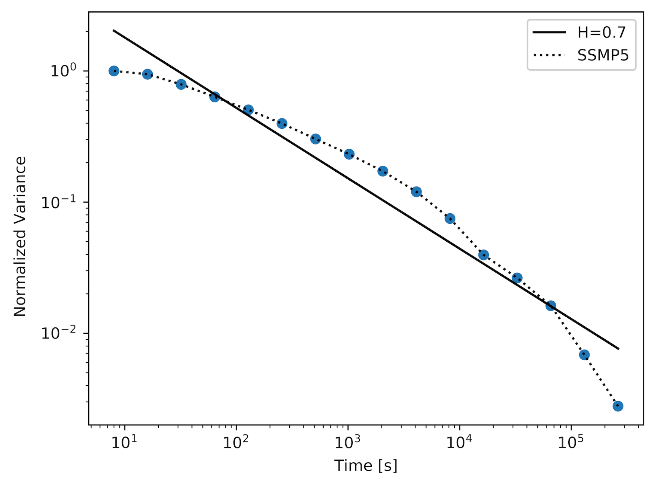
3). Note that for a steeper slope of the plot, the corresponding Hurst parameter takes smaller values. With the increase in the value of the slope, the value of the Hurst parameter decreases. The slope of the plot can slightly vary within a few first time-scales. This means that the value of the Hurst parameter within this range is non-identical for different time-scales. On the other hand, the visible decrease of the slope after the initial time-scales means that a process is no longer able to maintain self-similar properties. Such processes are self-similar only in a finite number of time-scales. We have fitted a straight-line for each of the plots using the least squares technique. At this point, it is necessary to mark that the values of the vertical axis differ between the figures. As a result, it is possible to observe that the slope of the straight-line fits differs between the figures. For every plot, we have computed the average and the maximum distance between a straight-line fit and the actual plot. The results of these computations have been presented in
Table 1.
For all three models, we wanted to produce traffic with at least . It was not possible for every Markov model to achieve a desired value of the Hurst parameter. To achieve such samples, it was necessary to repeat the experiment with modified parameters of the examined model. In the case of the SSMP model, we changed the number n of modulator states, and for MMPP model, we changed the number d of used active ON–OFF sources.
Figure 1,
Figure 2 and
Figure 3 show the results achieved using the SSMP model with a different number of states in a modulator (
n). For the model with
, which is the simplest model of its kind, the achieved approximated value of the Hurst parameter was
. The plot for this experiment is shown in
Figure 1. After increasing the number of states
n, it was possible to achieve a sample with a higher value of the Hurst parameter, which reached the value
. The corresponding plot is shown in
Figure 2. To achieve a sample with the desired value of the Hurst parameter, which was
, it was necessary to use an SSMP model with
. As we can observe in
Table 1, the maximum and average distance between the actual plot and the straight-line fit are decreasing with the increase in the number of states in the modulator. Returning to the three figures described above, we can observe that the number of time-scales for which the considered plots can have persistent linearity (and as a result, a stable value of the Hurst parameter) increases with the number of states in the modulator.
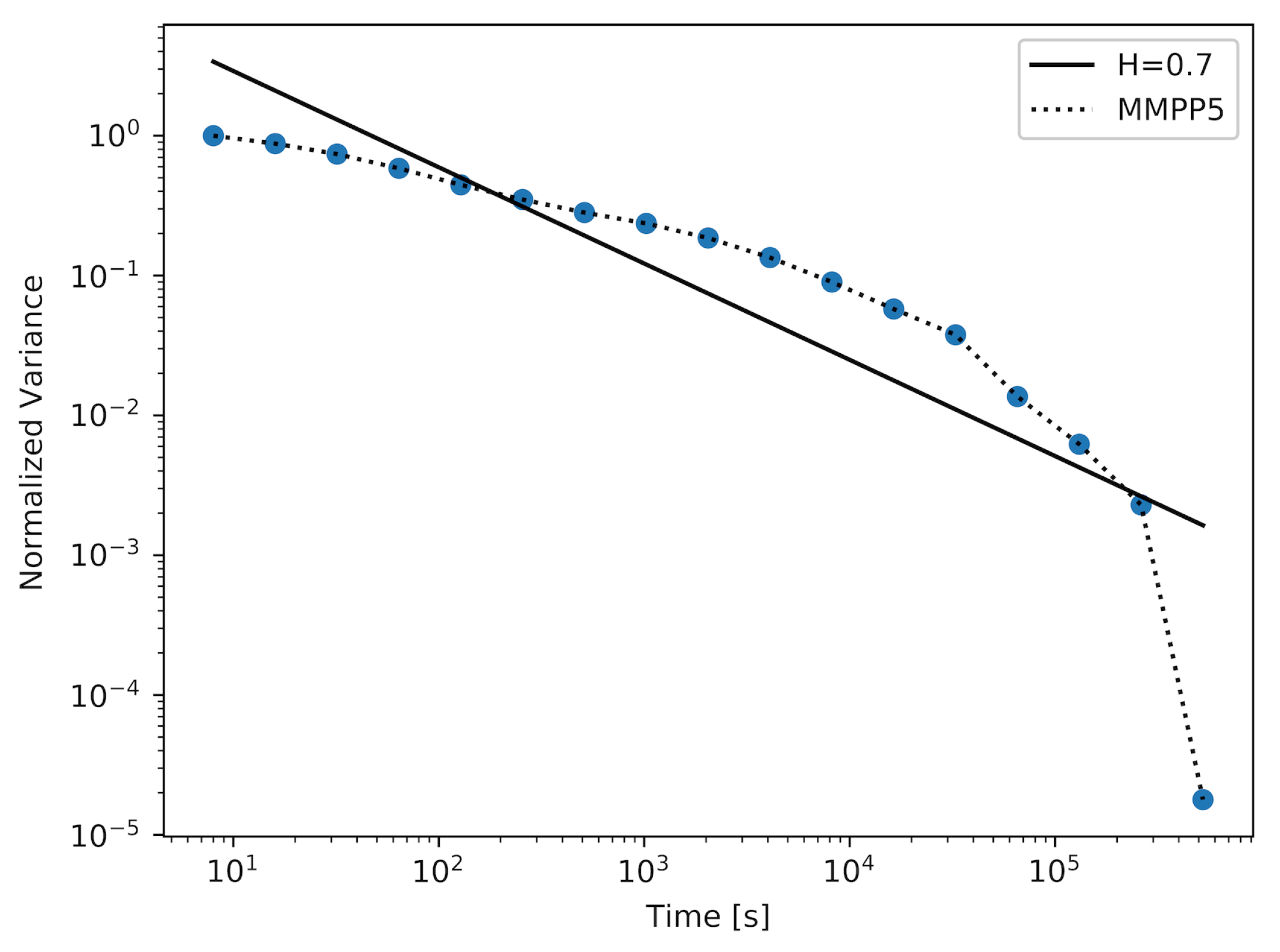
Figure 4 and
Figure 5 show the results achieved using the MMPP model with two different numbers of active ON–OFF sources (
d). For the MMPP with
, we were able to achieve a sample with
. The corresponding plot is shown in
Figure 4. It was necessary to increase the number of active MMPP sources to achieve samples with higher values of the Hurst parameter. In
Figure 5, we show the plot for the sample with
, which is a very high value of the Hurst parameter. We can observe in
Table 1 that, for a more complex MMPP model, the values of the average and the maximum distance between the straight-line fit and the actual plot decrease, which means that the approximation reflects the actual plot more closely.
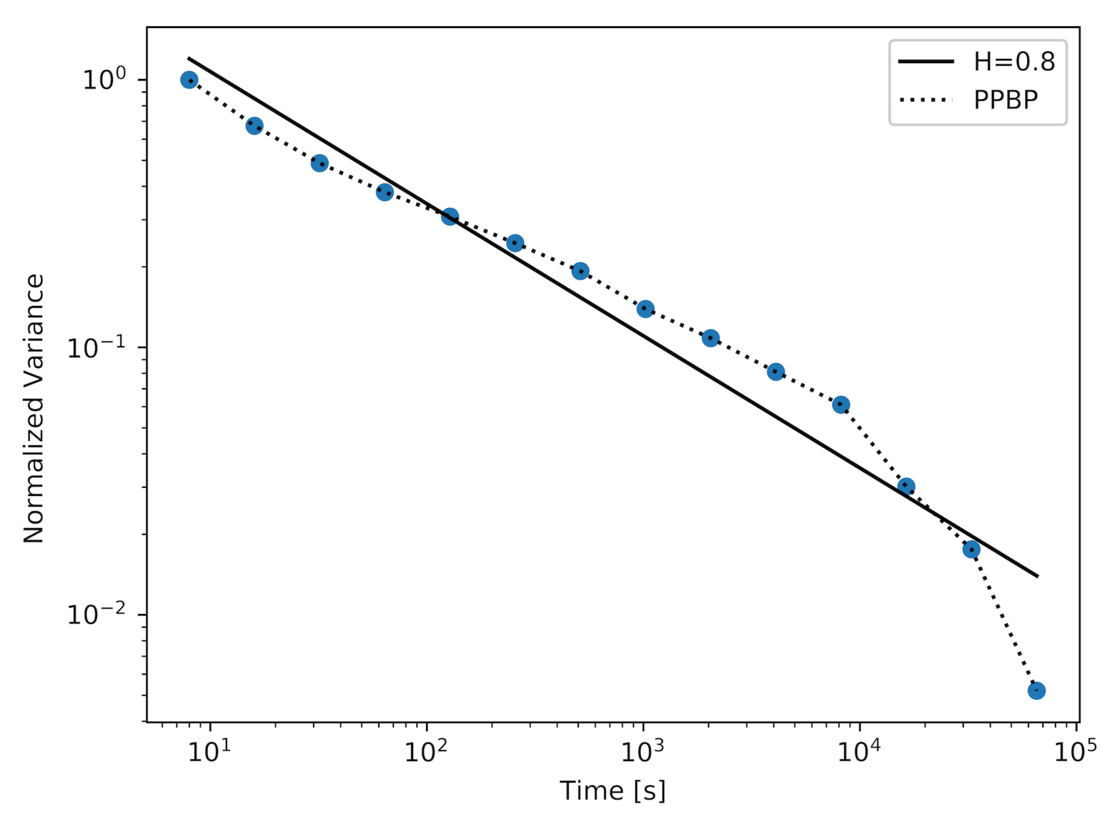
In
Figure 6, we present a plot for a non-Markovian model—PPBP. This is a model which is frequently used in network traffic analysis. The PPBP process consists of a simultaneous generation of packets by a larger number of Poisson sources. This number was changed during the experiment. Using this model, we obtained a sample with
. We can observe that the generated sample displays self-similarity over most of the measured time scales. The maximum and average distances between the actual plot and the straight-line fit for this model (presented in
Table 1) are the smallest.
The sample with the highest value of the Hurst parameter was achieved using a model with 22 active MMPPs. It is important to note that by generating this sample, the Markovian model has outperformed the PPBP model in terms of achieving the sample with the highest value of the Hurst parameter. We can also compare the plots achieved for these models (
Figure 5 and
Figure 6). The plot created for the MMPP model and its straight-line fit almost perfectly overlap for the majority of time scales, which means that the generated sample maintains a constant value of the Hurst parameter over these time scales. For the PPBP model, this overlapping is also visible.
All processes are not perfect self similar-processes but may imitate their features over the range of several scales, and this is sufficient for the needs of network traffic representation. In
Table 2, one can find a comparison of the time required to generate 1 million packets for the different examined models. With the increase in the complexity of the Markovian models (parameters
d and
n), we can observe an increase in the generation time. However, the time required to generate a sample for all the Markovian models is one order of magnitude shorter than for the non-Markovian model.
Note that the results of all three models were obtained here using the simulation. PPBPs can only be used in simulation models, unlike SSMPs and MMPPs, which may also be integrated with Markov queueing models. The usage of the Markov chains becomes intractable because of the number of states, which is rapidly increasing with the complexity of the modeled object. The introduction of self-similar sources increases the number of states, but we can cope with this issue by using the numerical methods described in
Section 2 for the larger models. Increasing the efficiency of the hardware also alleviates the problem.
4. Summary
The accuracy in creating Internet traffic models is crucial in the design and evaluation of secure and high-performance networks. It is necessary to understand the nature of Internet traffic to successfully optimize its performance and efficiency in the face of growing demands for fast information transfer. This can result in better job scheduling and resource management, ensuring the quality of transmission and preventing system malfunctions.
The network traffic exhibits self-similarity, which has a significant impact on network performance. The most well-known self-similar traffic models are not based on the Markov approach. Nevertheless, Markov models are traditional tools in the analytical evaluation of computer networks, and they should be adapted to the case of self-similar traffic.
A few Markov models can be used to create self-similar traffic sources. We have described two of them: the SSMP model using discrete-time Markov chains and the MMPP model using continuous-time Markov chains. Both of them enable us to obtain traffic that is self-similar in a finite number of time-scales. It has been shown that it is necessary to increase the number of states in a corresponding Markov chain (i.e., increase the size n of the modulator in the case of SSMP or the number d of sources in an MMPP) to produce traffic with higher values of the Hurst parameter. In this way, we also increase the number of time-scales for which the examined traffic may sustain a relatively stable value of the Hurst parameter and consequently self-similar behavior. These Markov models may also be used in simulations. We also compare these models with a non-Markovian PPBP model, which is widely used in simulations. A more complex MMPP model (with ) can successfully “compete” with a PPBP, not only in terms of the quality of provided self-similar process but also in terms of the efficiency of its generation: the generation time of a defined number of packets is several times shorter in case of an MMPP.
The great advantage of the Markov models is that they may be used in the modeling of transient states, which is important in the evaluation of computer networks as transmitted flows are continually changing due to the variability of transmissions and due to the performance of the flow control algorithms. The evaluation of transient states by simulation is extremely costly as it requires multiple repetitions. The biggest problem of the Markov approach is the large number of Markov chain states and consequently the high computational complexity. In the past, it was impossible to implement the more complex Markov models which are necessary to mimic real traffic data accurately. Due to the advances made in computing technology, complexity is no longer a problem, and Markov models can be successfully used in optimization tasks.

 ,
, 


