1. Introduction
Most indoor localization systems utilize some beaconing infrastructure (e.g., radio, light, sound sources) along with corresponding sensors to estimate various properties of the beacons (e.g., distance between the sensor and the beacon, angle of arrival and direction of the beacon, view angles between beacons, etc.). From the measured properties various location estimation methods can be used to produce the location estimates for the tracked object, which can be either a sensor or a beacon. In the first case, usually, multiple beacons are deployed at known positions and the sensor’s position is unknown, while in the latter case, multiple sensors are utilized with known positions to measure the unknown position of a beacon.
In this paper we focus on systems using angle of arrival (AoA) or angle difference of arrival (ADoA) measurements [
1]. Some of these localization systems use acoustic sources [
2,
3], an interesting example being weapon localization where the beacon is the muzzle blast of the weapon [
2], but the majority of AoA/ADoA systems utilize optical sources, e.g., blinking LEDs [
4,
5,
6,
7,
8,
9,
10,
11,
12,
13]. In such systems bearings are measured between the sources and the sensors, and based upon the angle measurements the unknown location is estimated using various means, e.g., least squares estimates [
4], consensus functions [
5], or exhaustive search [
4].
The direction of a beacon can be measured in three dimensions (3D), when two angles, the azimuth and the elevation, are determined, or in two dimensions (2D) only, when one angle, the bearing (i.e., azimuth), is measured. The 3D approach allows localization in 3D with arbitrary sensor orientation, while 2D measurements can be utilized when certain constraints are fulfilled, namely in this case the sensor orientation must be either measured or known (typical use case is when the sensor is heading upwards) [
4,
5]. The main advantage of the 2D approach is that the computational complexity can be decreased significantly [
6]. The measurement method proposed in this paper provides 2D bearing measurements.
For the measurement of bearings of light sources image sensors (e.g., cameras) can be utilized. The tilting of the sensor can be either measured by auxiliary sensors [
4,
5] or can be estimated from the image itself [
7,
8].
Light sensors (e.g., photodiodes) offer a more cost-effective solution; such devices utilize the directional sensitivity of the light sensors. The quadrant photodiode angular diversity aperture (QADA), which utilizes four specially arranged photodiodes on a plane, with an auxiliary aperture was proposed [
9]. Traditional photodiodes (PDs), arranged in various geometrical formations were also proposed to measure bearings: in [
10] and [
11] the PDs were attached on the edges of a cube, while the planar circular photodiode array (PCPA) utilizes PDs placed on the surface of a cylinder [
12,
13].
In this paper the performance properties of the PCPA are analyzed. The PCPA was proposed with a corresponding least squares (LS) bearing estimation in [
12]. The hardware architecture was improved in [
13]. In this paper a novel computationally efficient bearing estimation, using frequency domain, is proposed. The performance of the measurement methods in the presence of various physical error sources is analyzed. The results demonstrate that the effect of reflections can be significant, while the tilting of the sensor has only minor effect on the bearing estimation. The applicability of the measurement device in indoor localization applications is illustrated by real localization examples.
2. The Planar Circular Photodiode Array (PCPA)
2.1. Background of Operation
The operation of the proposed method is based on the directional sensitivity of the photodiodes.
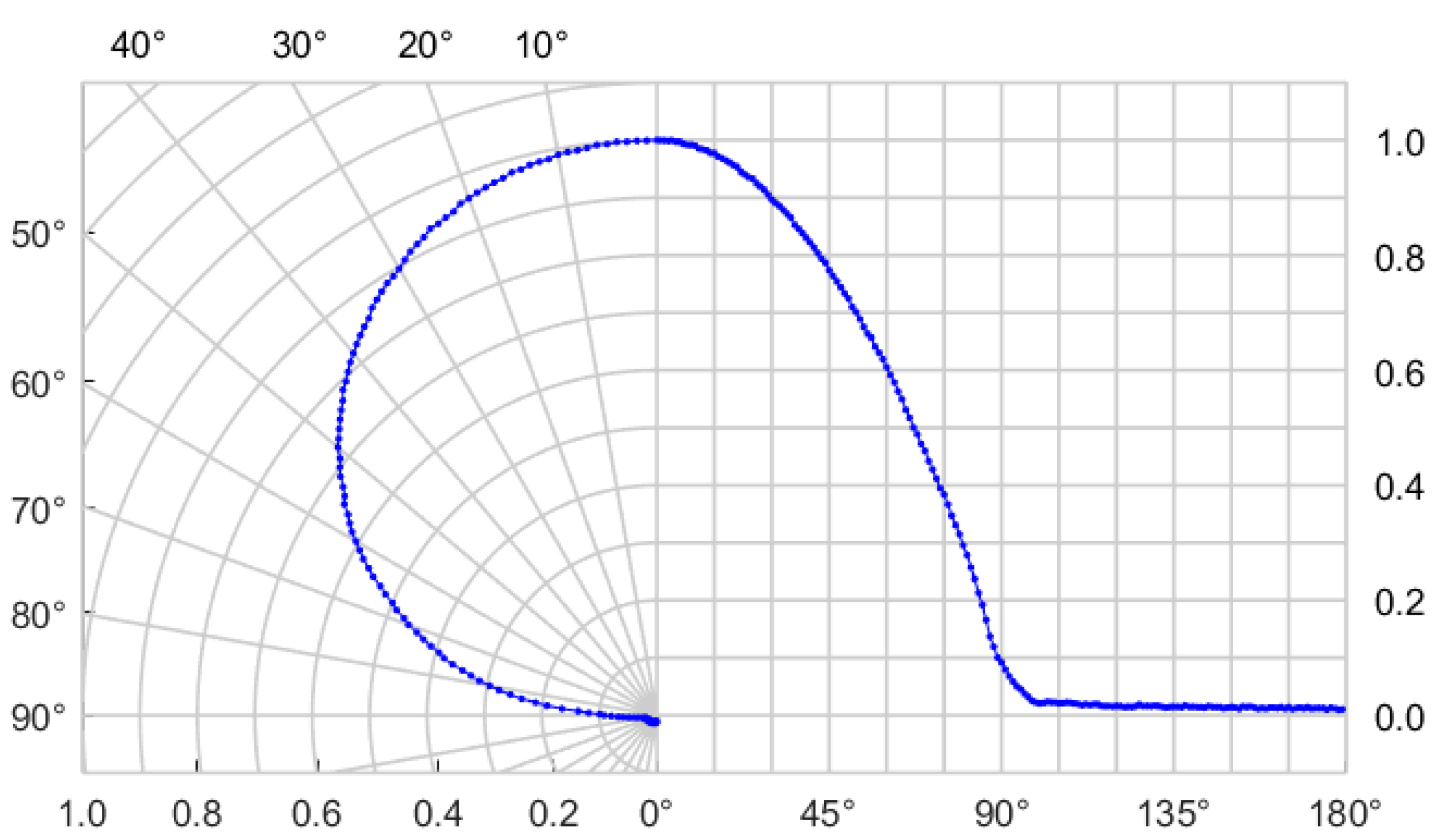
Figure 1 shows the measured normalized angular response of a photodiode, type SFH205F [
14], as a function of angle
of the incoming light. The left-hand side is shown in a polar system, while the right-hand side in a Cartesian coordinate system. Notice that the maximum sensitivity value was set to unity, hence the name normalized. Apart from the direction, the detected light intensity (i.e., the current flowing through the photodiode) also depends on the emitted light intensity and the distance between the source and the sensor.
Using multiple photodiodes, the dependence of the distance and the source light intensity can be cancelled, thus angle can be measured. Our goal was to create a sensor and a corresponding measurement method which can determine the angle of the incoming light in 2 dimensions. Thus it is supposed that the light source and the sensor are placed (approximately) on the same plane. The proposed measurement setup will be introduced in the next Section.
2.2. Measurement Method
The measurement setup is shown in
Figure 2. The system contains beacons
, which are infrared transmitters, each of which having a unique blinking frequency, which allows the separation of the beacon signals in the measurements. The PCPA consists of
PDs arranged evenly along a cylinder, facing outwards, thus the angle between neighboring channels is
. The beacons and the PCPA are assumed to be approximately on the same plane.
Notice that each PCPA channel measures the additive incoming light intensity, coming from all beacons. The beacons’ signals are separated in the frequency domain by the digital signal processing unit [
12] and the detected amplitude of each beacon is measured by each channel. Using the measured intensities the bearing
of each beacon
is determined. A least squares (LS) and a fast frequency domain (FD) method will be introduced in
Section 2.3 and
Section 2.4, respectively.
2.3. Least-Squares Estimatior
The least-squares angle estimate is reviewed here based on the results of [
12] and [
13]. The incoming light intensities from a particular light source are measured and the
-element measurement vector denoted with
, as follows:
where
is the measured light intensity in channel
and
is the transpose operator.
A calibration matrix
is created where
is the number of channels in the PCPA and
is the number of calibration measurements. Row
of
corresponds to a particular PCPA channel
, and the values in this row contain the measured channel sensitivity values, sampled in
equidistant angles
,
, where
Notice that
Figure 1 contains such a normalized measurement for one channel. See
Section 4.1 for further multichannel measurement examples.
On the other hand, columns of
correspond to directions
, as follows:
where column
contains intensity values
for each channel
, measured using a light source with bearing
The least squares bearing estimate will be the angle
for which the shape of
is closest to the shape of
, in the least squares sense. Recall that the measured light intensity depends not only on the bearing but also on the distance between the light source and the sensor, and also on the power of the light source. Thus we use a scaling in order to define the distance between
and
as follows:
In (5)
is the squared error between the calibration vector
and the measured vector
, and
is the unknown scaling factor. The least squares cost function for angle
is defined as the smallest possible value of
as follows:
As a first step, we determine the optimal value for
, given the value of
. From (2) and (3) it directly follows that
At the minimum of
the derivative
is zero:
From (8), the optimum value of
is the following:
Using the optimal value of
, the cost function (6) now can be calculated as follows:
Notice that each index
corresponds to bearing
Thus index
, for which the cost function (9) is minimal, defines the best bearing estimate. The optimal bearing index
is the following:
and, using (2), is the bearing estimate is
Notices:
- (1)
The resolution of the bearing estimate (11) is
, i.e., the higher
is, the better the resolution. Observing
Figure 1, it is apparent that the sensitivity curves are smooth, which enables interpolation between measured values. The sensitivity value
for an arbitrary angle
, for which
, can be calculated as follows:
Using (13), the size of the stored calibration matrix can be kept low, while the resolution can arbitrarily be increased.
- (2)
The computational complexity of the least squares estimate as follows: the calculation of requires approx. operations (multiplications, divisions, additions, and subtractions). The brute force minimization requires the calculation of calculations, while a gradient search requires operations, where is the number of gradient search steps. In practice may be smaller than , but the number of calculations is still at least an order of magnitude higher than . In the current implementation the calculation of a bearing estimate requires 150 ms in a PC-class computer. Thus the implementation of the LS estimator is troublesome on low-scale microcontrollers.
2.4. Fast Angle Estimation in the Frequency Domain
To overcome the high computational complexity of the LS estimator, described in
Section 2.3, a fast computation method will be proposed, where the angle estimation is made in the frequency domain.
The following assumptions are made:
The relative sensitivity characteristics of the individual PCPA channels are almost identical. The universal normalized sensitivity characteristic is , where is periodic with ;
The sensitivity characteristics are even symmetrical.
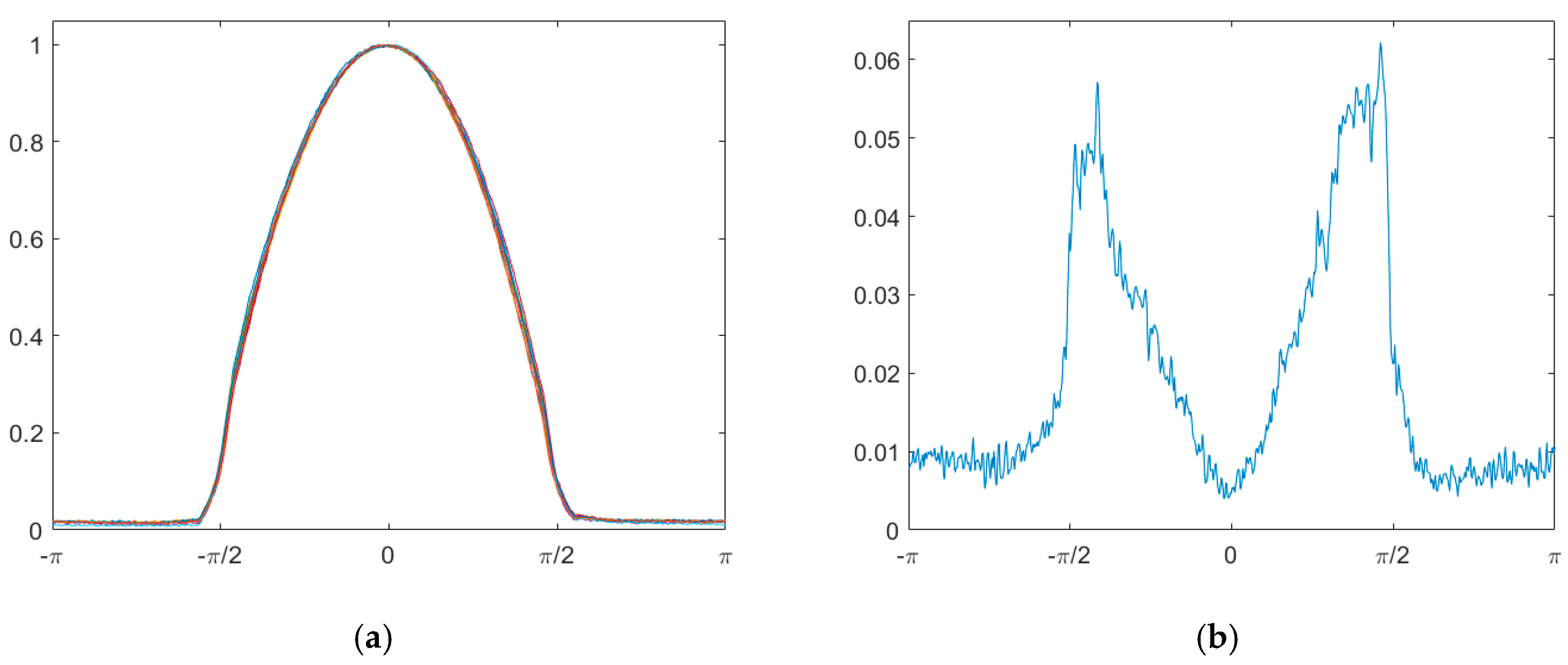
The justification of the assumptions can be seen in the measurements shown in
Figure 3.
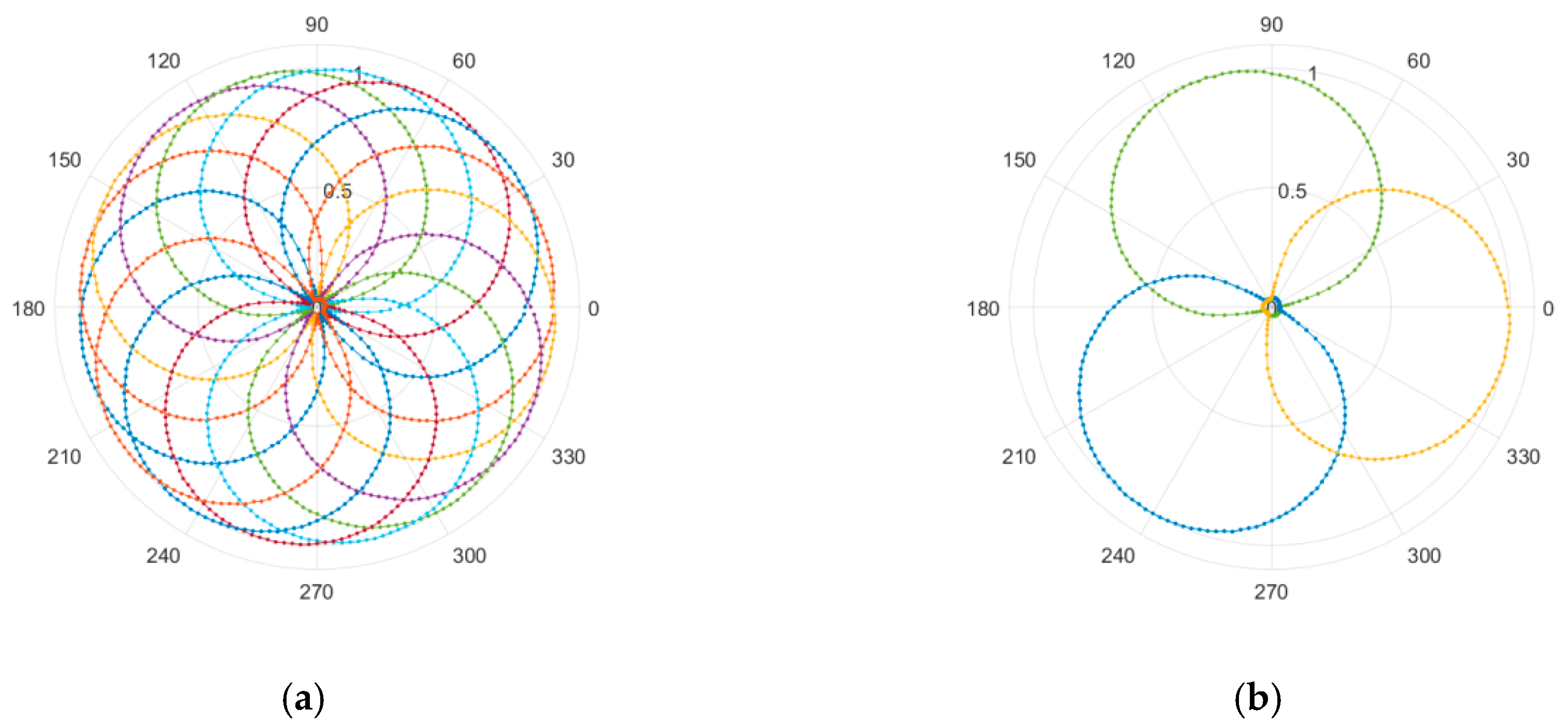
Figure 3a shows the normalized sensitivity characteristics of 16 PCPA channels (these are in fact the radial sensitivities of the applied individual photodiodes), while
Figure 3b shows their maximum difference between the measured normalized sensitivities. As the figure shows, the difference is indeed small; this is expected since the same type of photodiode was used in each channel.
Figure 3a also shows that the sensitivity curve is indeed even symmetrical.
Since the channels are rotated by
(see
Figure 2), the incoming light angle, coming from the same source, changes by
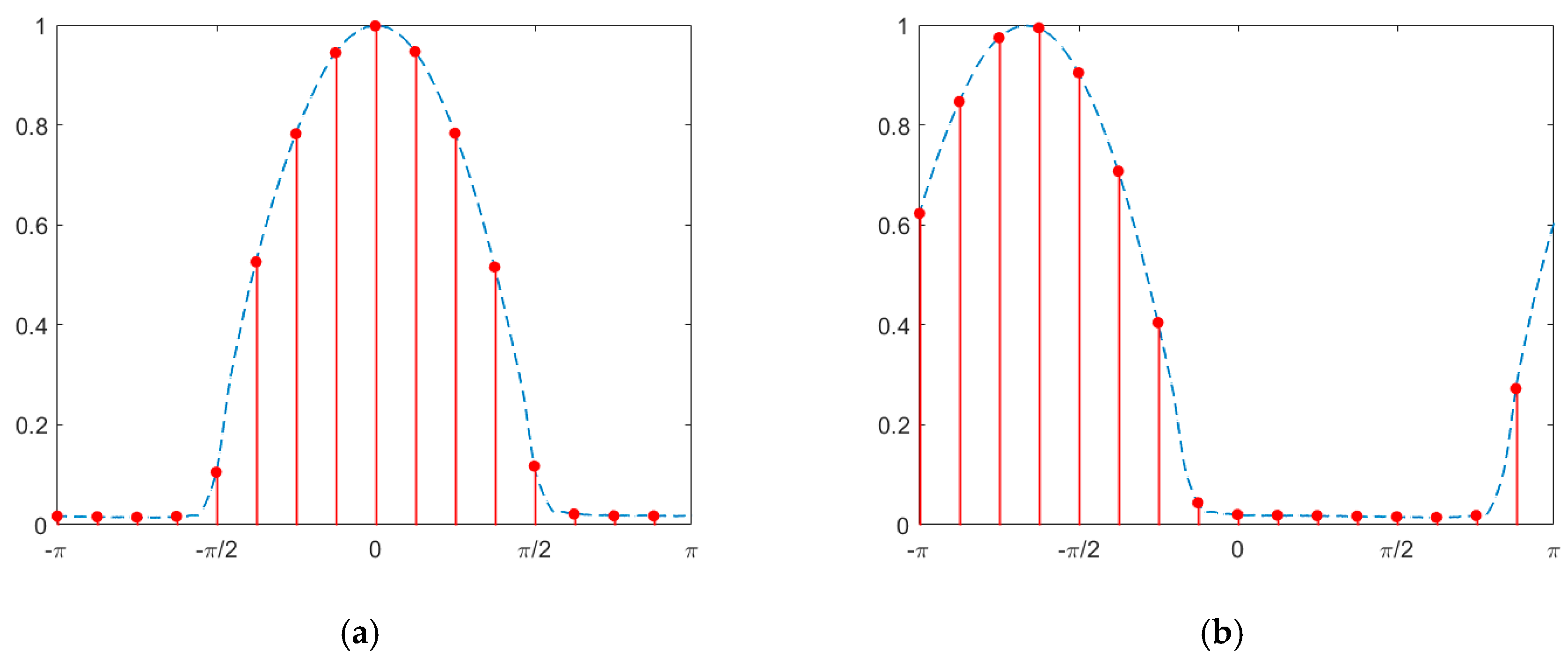
at each channel. Thus the
(
values, provided by a measurement, can be considered as equidistant samples of the
sensitivity curve, as follows:
The measurement, modeled as a sampling process, is illustrated in
Figure 4, for incoming angle values of
= 0
and
= −120
, for the photodiode shown in
Figure 1. The
–element sample vector, as a function of
, is denoted by
. The angle estimation should determine the value of
, from the measured vector
The case when the light source is in direction zero, i.e.,
as in
Figure 4a is examined.
is the DFT of the sampled sensitivity curve
, as follows:
Since
is even symmetric,
is real, i.e., the angle of all harmonic components in
, including the fundamental harmonic
, is zero. In considering a case of an incoming light with arbitrary angle of
, where the DFT of
is
:
Using the shift property of the DFT, the value of the fundamental harmonic
of
can be expressed as follows:
Since
is real, the angle of
is
Thus, the frequency domain (FD) angle estimation can be carried out in the following way: First calculate the first harmonic component of the DFT of the measured vector
, as follows:
where
Then the angle estimate
is the following:
The computational demand of the fast method is only approx. (real) operations, which is significantly smaller, than that of the least squares estimate.
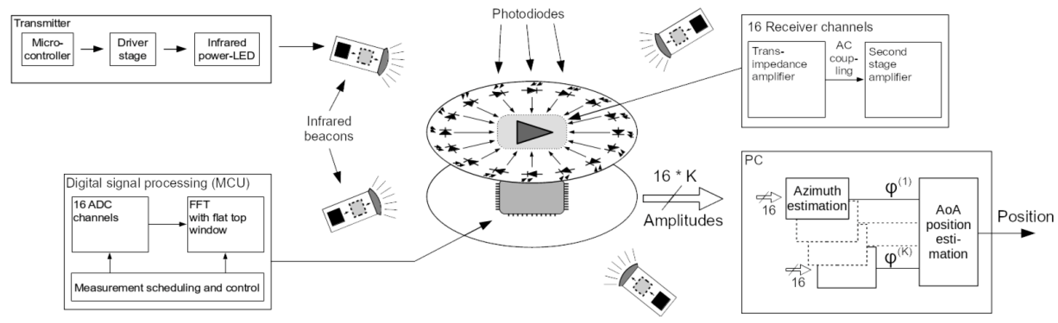
3. Measurement System
The architecture of the measurement system is shown in
Figure 5. The beacons generate infrared light, blinking with unique frequencies. The beacons contain a PIC12F1572 microcontroller, a driver stage and a high power infrared LED. The illustration of
Figure 5 contains
beacons.
The current implementation of the PCPA consists of
photodiodes. These SFH205F types have a cylindrical front side [
14]. Each of them is followed by a two-stage transimpedance amplifier, providing fourth order lowpass filtering and 130 dBOhm gain. After multiplexing, the amplified and filtered signals are sampled and converted by the internal analog-digital converter of the PIC32MZ2048EFM064 microcontroller with 40 kHz/channel. The spectra of the 16 signals are calculated by the microcontroller with fast Fourier transform using a flat top window and a transform size of 1024. For each beacon, the amplitude, corresponding to the beacon frequency, is measured on each channel, thus the PCPA provides
amplitude values with an update frequency of 39 Hz.
The second processing step is currently performed on a PC, where the bearing estimates are computed using either the LS or the FD estimate, as described in
Section 2.3 and
Section 2.4, respectively. The current LS estimator can provide bearing values with 6 Hz on a PC, while the FD estimator’s update frequency is higher than 1000 Hz. The execution time of the FD estimator, implemented and optimized on the microcontroller, is approx..
.
The bearing measurements are then used to estimate the position of the sensor. Using the known beacon locations and the measured bearings the position estimation can be computed by any AoA/ADoA method, e.g., exhaustive search [
4], consensus functions [
5], geometric methods [
6], or LS methods [
4] may be utilized The location estimates on the PC can be calculated to provide an update for each bearing measurement (i.e., with 39 Hz).
The photo of the PCPA is shown in
Figure 6. The PCPA sensor (photodiodes) is a cylinder with diameter of 38 mm and height of 20 mm. In the current implementation the analog and digital electronic circuits are located on two circular PCBs with diameter of 100 mm (no attempt to optimize the size was made). The photo also shows the turntable, used in the measurements.
Both the beacons and the sensor are of low cost: the bill of material (BOM) cost is USD 14 per beacon (including main power supply), and USD 30 per receiver.
4. Measurements and Evaluation
In this section measurements are presented to analyze the sensitivity of the PCPA to two practically important error sources. The first error source is reflections: the beacon signals may be reflected from various surfaces near the PCPA, thus not only the line of sight signals, but other disturbing components will be measured, causing error. The second possible error source is the tilting of the sensor: in practical scenarios the sensor’s alignment may not be perfect, thus the not homogenous vertical sensitivity of the applied PDs may cause error.
In the subsequent sections, first the reference measurement is introduced. The impact of the error sources will be analyzed on
- −
raw measurements, i.e., the measured light intensities (
Section 4.2),
- −
- −
and finally, localization results in some illustrative scenarios (
Section 4.4).
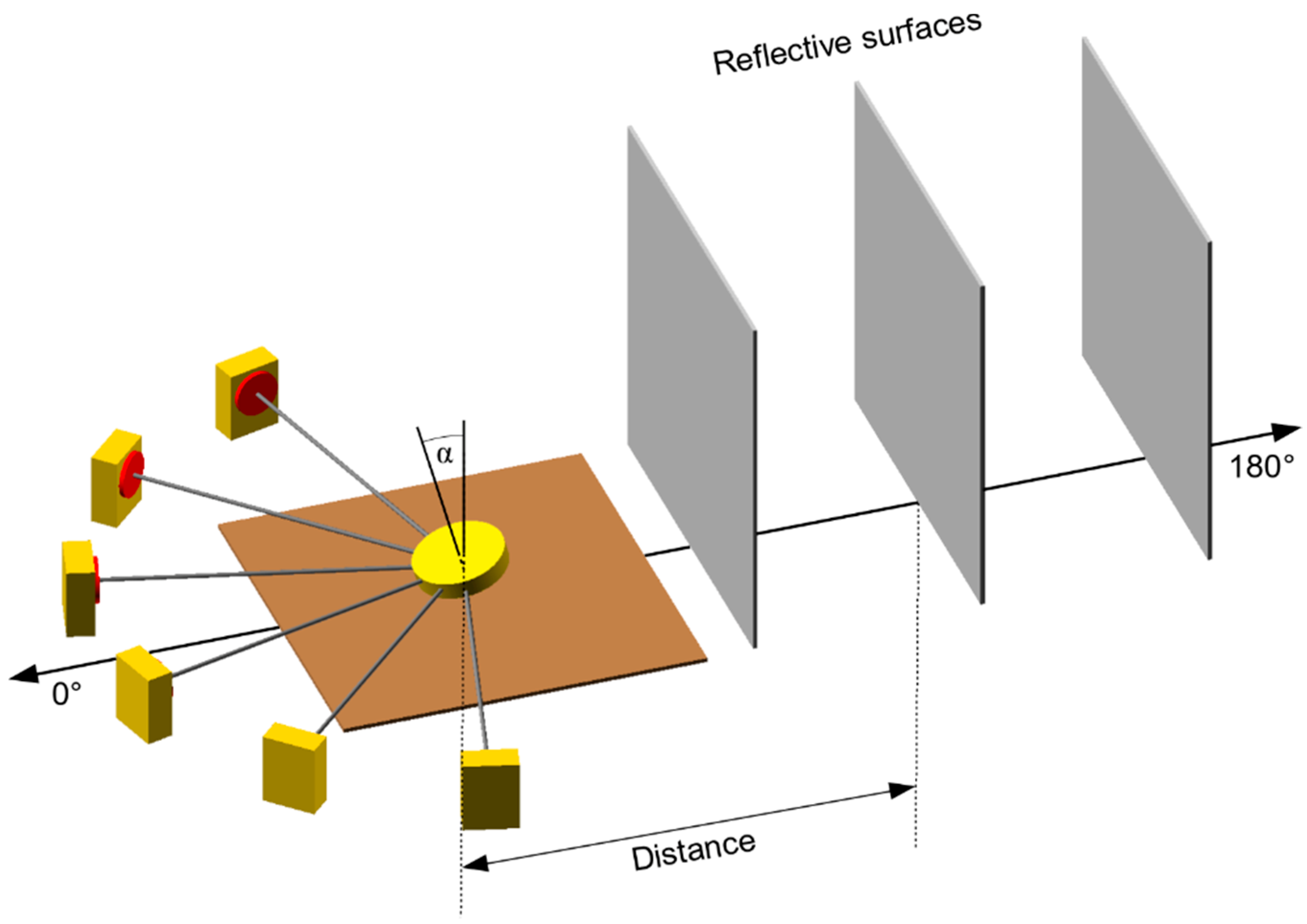
The generic test setup can be seen on
Figure 7. The center piece is the PCPA itself, which was placed on a turntable. With this turntable the measurement device could be accurately rotated around the vertical axis. Ideally the PCPA’s normal vector is vertical, but to investigate the effect of tilting, the PCPA may be mounted on the turntable with various tilting angles, denoted by
in
Figure 7. The turntable allowed the measurement of the radiant intensity characteristics automatically with a resolution of 1°.
The beacons were deployed on one side of the PCPA, around direction zero, as shown in
Figure 7. On the other side of the PCPA (in direction 180°) various reflective surfaces were placed at different distances from the PCPA. The reflective materials, including white paper, black paper, aluminum foil, and mirror, were placed on 80 × 80 cm wooden surfaces.
It is important to note, that the measurements were carried out in a 5 m × 4 m office, which was furnished and had several large white areas on the walls. Thus some of the measurements may include the influence of the reflections of the environment.
4.1. Reference Measurement
The LS estimator requires the reference matrix , which contains the reference intensity characteristics of each channel. Recall that each row of corresponds to a channel, while each column corresponds to a bearing. The values of can be produced by a measurement, carried out as follows. A beacon was placed in front of the PCPA, at direction of 0°. To minimalize the effects of reflections a black foam was placed on the opposite side of the PCPA (between directions of (−90°)–90°, and the beacon was placed in a tube pointing to the measurement device.
During the measurement, the PCPA was rotated with the turntable with a resolution of 1°, while the light intensity was averaged from 20 measurements at each angular position. For better visibility, the data corresponding to each channel were normalized. The results of the measurements can be seen for all the 16 channels, and the three selected channels in
Figure 8.
Note, that the resolution of the reference matrix
can be increased with interpolation, as described in
Section 2.3. Additionally, note that the resulting characteristics are relatively “smooth” and almost identical (see also
Figure 3, showing the same measurements).
4.2. Light Intensity
In the case of the reference measurement we strove to eliminate environmental factors, mainly reflections. However, it is interesting and also crucial to know what kinds of deviations are produced in the measurements in non-ideal conditions. In this chapter the effect of reflective materials and the tilt of the PCPA are be analyzed on the recorded light intensities.
4.2.1. Effects of Reflective Surfaces
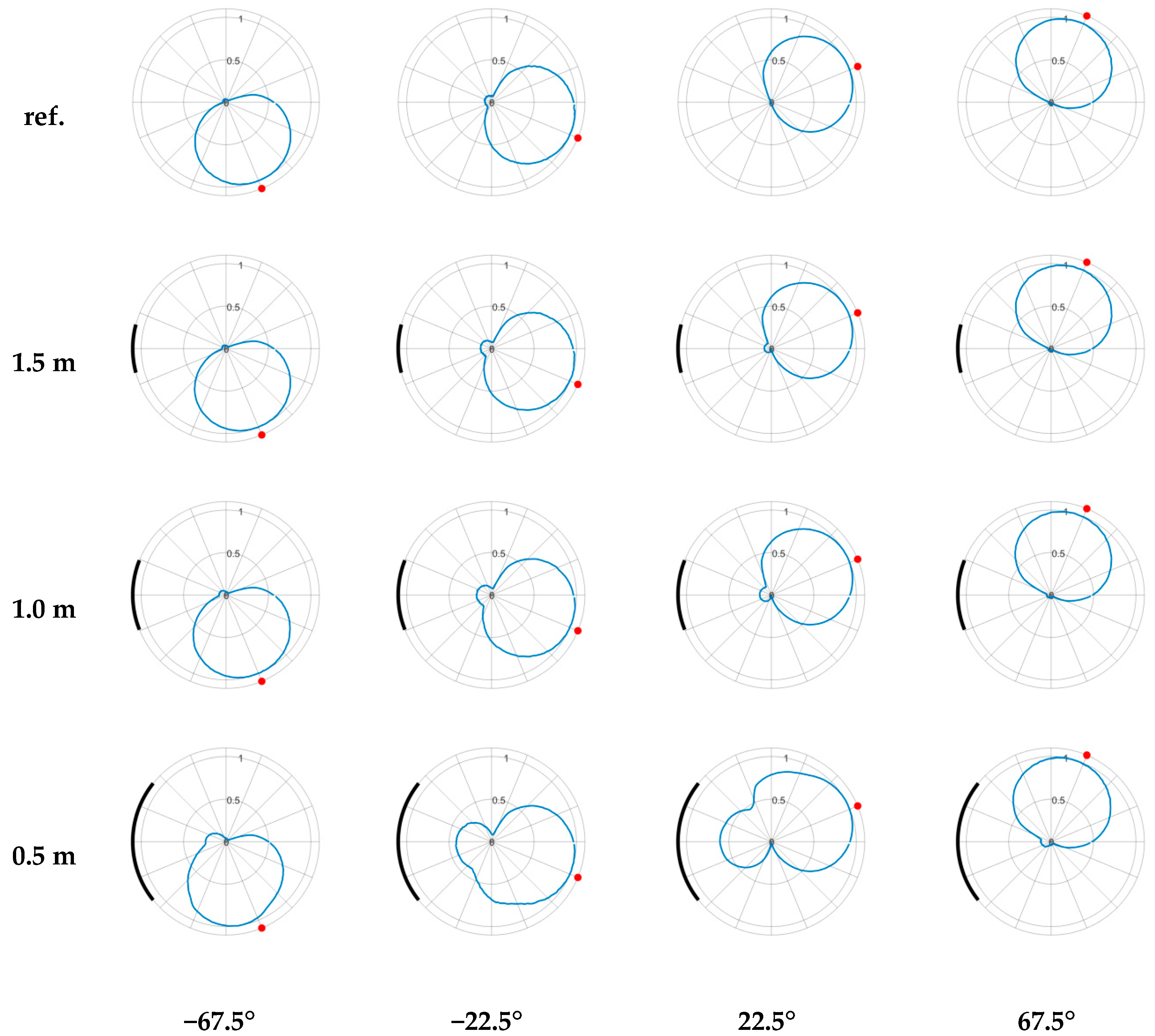
For examining the effect of reflecting surfaces, a series of measurements were conducted utilizing the test setup depicted in
Figure 7. In the measurements four beacons were placed at ±22.5° and ±67.5°, and an aluminum foil was used as a reflective material. The reflective surface was placed at 0.5, 1.0, and 1.5 m from the center of the PCPA. During the measurements, the PCPA made a full rotation with a resolution of 2°, and the light intensity values were recorded at each angular position.
In
Figure 9 the results of the experiments can be seen, where the blue lines represent the normalized light intensity values of the measurement channel facing 0°. The angular placements of the beacons are represented with the red dots while the reflective surface is always at 180°, denoted by a black arc; the length of the arc representing the viewing angle of the surface (the higher the distance between the surface and the PCPA the smaller the viewing angle). The first row of the figure represents the reference measurement where no artificial reflective material was present (but some unwanted reflection from the walls still may be present here).
In
Figure 9 several trends can be clearly seen: with decreasing distance between the PCPA and the reflective surface the deviations from the ideal (reference) characteristic are increasing. The most prominent abnormality is the bulb-like shape, created by the reflection of the beacon. In these angular positions the measured values should be zero because the photodiode at these positions is facing backwards, thus no direct line-of-sight is present.
It is important to note that the measurement shown in
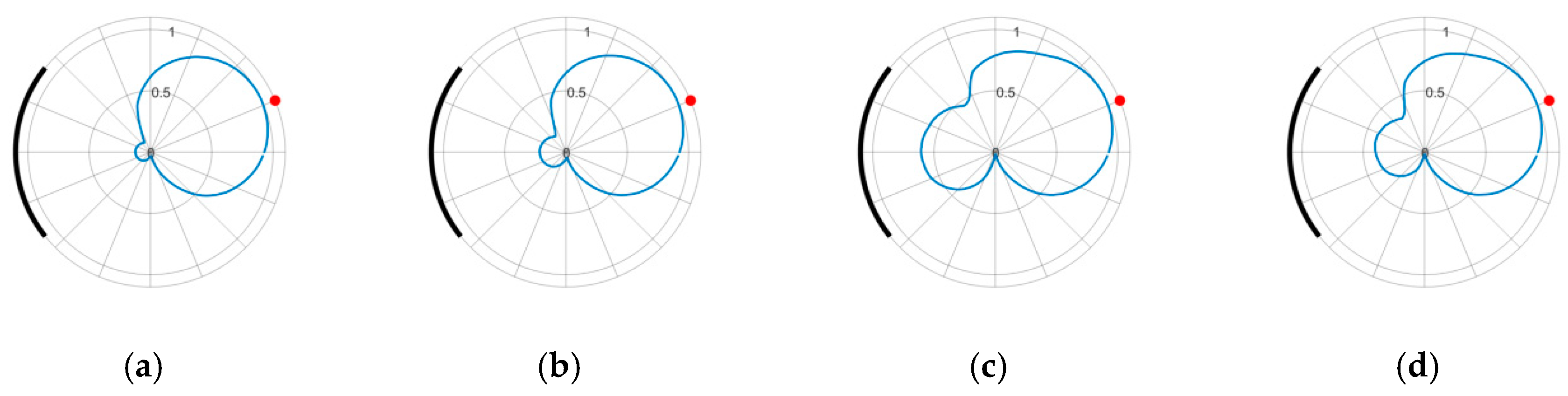
Figure 9 is an extreme and conspicuous case of reflectivity, where a large piece (80 cm) of aluminum foil was used. For comparison,
Figure 10 shows measurements of different materials with the same setup at a distance of 0.5 m. From the measurements it shows that the aluminum foil may have greater impact than the mirror (at least in the setup shown in
Figure 10), probably due to the combined effect of reflection and scattering. Black paper has a minor, but still visible, effect, while white paper also shows significant impact.
4.2.2. Effects of PCPA Tilt
In principle, the PCPA was designed with the assumption that both the beacons and the utilized photodiodes are aligned on a plane, i.e., the normal vector of the PCPA is vertical. However, in real world applications (e.g., localization of a mobile robot platform) the PCPA may be tilted. Thus it is important to analyze the deviations caused by a small amount of tilt.
In our experiments we utilized the setup and rotation pad depicted on
Figure 6. The PCPA was assembled with multiple mounts, which provided a tilt of 0°, 1°, 3°, 5°, and 10°.
The results of the measurements can be seen on
Figure 11, where the maximum absolute amplitude errors are plotted relative to the 0° tilt measurement values. The exact utilized error function was derived as follows. The measured not-normalized sensitivity characteristics of channel
, measured at bearing
, using tilt angle of
, are denoted by
. The reference measurement is
, which is shown in
Figure 8. The measurement error
at bearing angle
, caused by the tilting of the sensor, is defined as follows:
Notice that in (22) the first term is the normalized reference sensitivity characteristics of channel
, while the second term is measured with the tilted sensor using the same (reference) normalization factor. Thus (22) provides a metric to characterize the measurement error, due to tilting.
Figure 11 shows the measured
values for
.
As
Figure 11 shows, the largest error is expected in directions toward the tilt, i.e., in our case towards directions 0° and 180°. The error is small in directions perpendicular to the tilting direction, in this case 90° and 270°. It should be noted that the error never reaches 0 and a small asymmetry is also present, due to the measurement and processing noise and a minimal reflection from the environment. Additionally, it is notable that the
tilt for the PCPA is an exaggerated case: most of the intended applications for the device provide less deviation (e.g., in case of industrial mobile robots the tilt is limited by the maximum inclination of ramps).
Based on the results shown in
Figure 11, it is evident that the effect of the sensor tilt is negligible to the measured amplitude values (mostly below 5%) compared to the deviations caused by reflective surfaces (e.g.,
Figure 9 and
Figure 10, where the deviation can be as much as 10%–660%).
It is important to note, that the relatively low amplitude variations caused by the tilt of the PCPA is due to the shape of the photodiodes. The selected type has a cylindrical front side, in contrast to the most common half sphere shape, providing smaller vertical sensitivity.
4.3. Bearing Estimation
The next stage of the processing chain is the bearing estimation phase. In this section, the effect of the reflections and the tilt of the PCPA will be examined to the angle estimation. In the evaluation, both the LS and the FD estimation methods will be utilized and the results will be compared.
4.3.1. Effects of Reflective Surfaces
Measurements with reflective surfaces were conducted utilizing a measurement setup similar to the one shown in
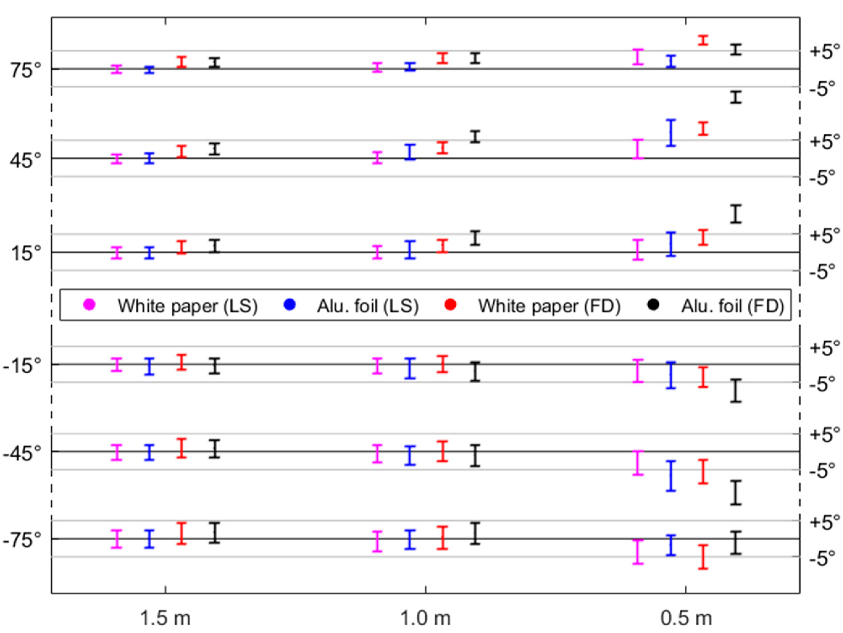
Figure 7, but in this case six beacons were used at the angular positions of ±15°, ±45°, and ±75°. During the measurements full rotations were made with resolution of 2°. As a reflective surface, white paper and aluminum foil were assembled on an 80 × 80 cm board. The distances of the reflective materials in the measurements were set to 0.5, 1.0, and 1.5 m.
The measured angle estimation errors are shown in
Figure 12, while the numerical values can be seen in
Table 1.
As the results show, by decreasing the distance between the PCPA and the reflective material the error of the estimated angle increases. The proximity of the reflective surface increases the bias of the calculated angle, the direction of the error also depending on the angle between the beacon and the reflective material. The FD estimator clearly shows higher bias compared to the LS estimator, while the standard deviation of the measurements are similar. In worst case (aluminum foil at 0.5 m), the mean error was as much as 4.3° for the LS, and 9.3° for the FD estimator. For realistic cases (distance 1.5 m) the error is around 1° and 2° for the LS and FD estimators, respectively.
4.3.2. Effects of PCPA Tilt
To analyze the angle estimation error caused by the tilt of the PCPA we conducted multiple measurements. In our experiments we utilized the setup and rotation pad depicted on
Figure 6 and
Figure 7. The PCPA was assembled with multiple mounts, which provided tilt values of 0°, 1°, 3°, 5°, and 10°.
The bearing estimation errors can be seen in
Figure 13, where the errors are plotted for both the LS and FD estimator. The errors were defined as the differences between the bearing estimates using the 1°, 3°, 5°, and 10° tilted measurements, and the bearing estimates using the 0° tilt reference measurement.
As
Figure 13 shows, the angle errors due to the tilt of the PCPA are negligible, usually below 0.25° (except the 10° case), which is the same magnitude as the measurement error of the current system. Note, that reflective surfaces cause several times higher angle estimation inaccuracies.
4.4. Localization Measurements
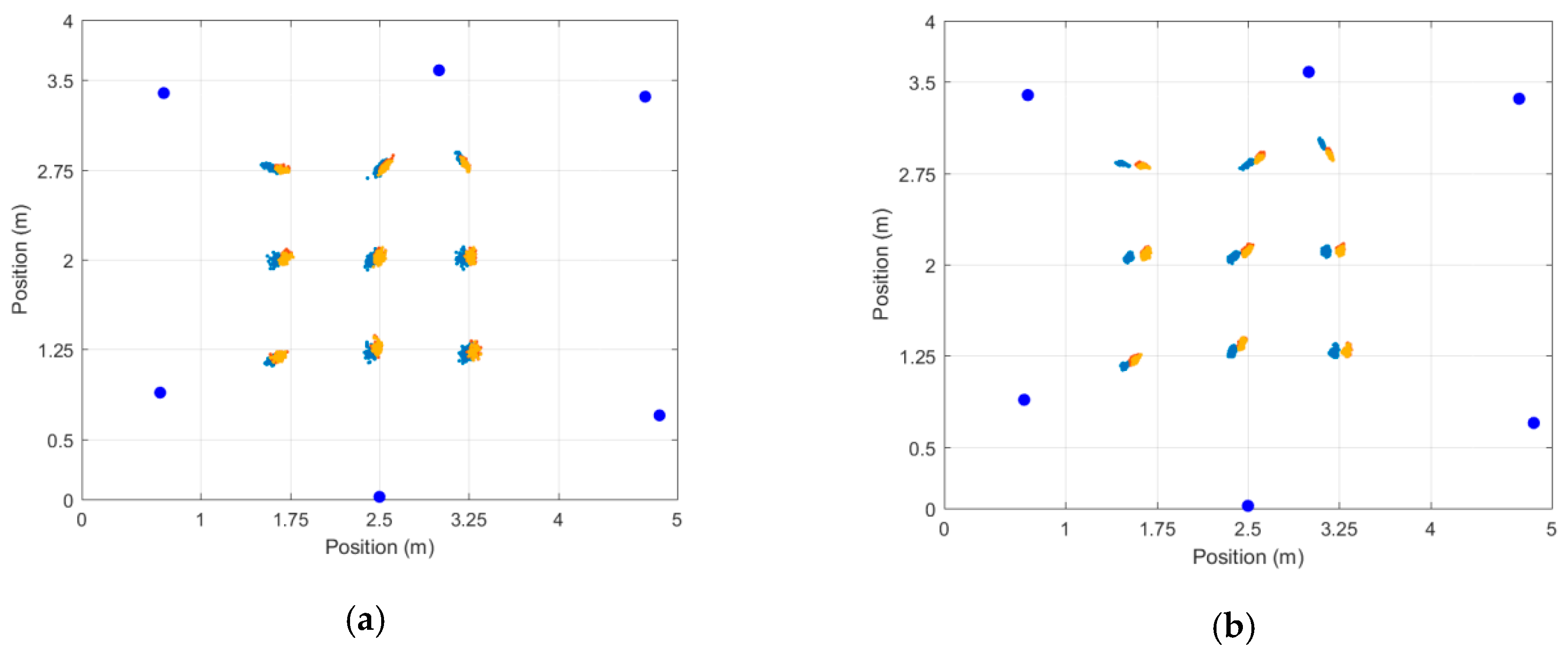
To illustrate the potential application of the proposed bearing measurement method an indoor measurement setup was built. In this section, the performance of the system is analyzed through the localization accuracies with various amounts of reflections and tilt.
The system was installed in a 5 m by 4 m furnished office room, with several white areas on the walls. The measurements utilized five or six beacons as anchor points. The nine reference positions were on the grid shown in the center of
Figure 14. At each reference point the sensor was rotated, taking 72 independent measurements. From the measured bearing values, the sensor position was estimated using a least-squares ADoA-based position estimator.
4.4.1. Localization with Various Amounts of Reflections
In our first experiment, six beacons were utilized. At each reference point, two independent measurement runs were made: a “normal” measurement with no artificial reflections, and a measurement with white paper placed next to the PCPA (50 cm to the right) as a reflective surface. The placement of the beacons and the measurement results can be seen in
Figure 14, utilizing the LS and the FD methods for bearing estimation.
The statistical results of the experiments are presented in
Table 2, where the localization accuracies are also calculated for a case where only four beacons are present. In these scenarios the measurements of the top and bottom beacons are excluded from the localization.
As can be seen in
Figure 14 and
Table 2, the localization accuracy based on the LS estimator outperforms the FD estimator in similar cases. This is probably due to the bias caused by the reflections of the environment, to which the FD estimator is more sensitive than the LS estimator (see
Figure 12).
It is noteworthy that the white paper placed right to the reference positions are clearly biased the position estimates to the left. Without artificial reflections, which can be considered “normal” operation condition, the accuracy of the systems is around 7–8 cm for the LS, and 14–16 cm for the FD estimator. The effect of artificial reflections is clearly higher when the number of beacons is only four (since the redundancy is small), resulting in 15–28 cm of mean error; while for the six-beacon case the effect is smaller (due to higher redundancy), increasing the error to 10–18 cm.
4.4.2. Localization Width Tilted PCPA
Another localization experiment was conducted utilizing five beacons, with a similar beacon arrangement as can be seen in
Figure 14. The purpose of the measurements was to quantify the localization error caused by the tilt of the PCPA.
Table 3 summarizes the statistical results of the experiments.
As the data in
Table 3 indicates, the tilted and non-tilted measurements are almost identical. This indicates that the utilized hardware, more precisely the cylindrical shape of the photodiode is highly tolerant to the tilt of the PCPA.
5. Conclusions
Planar circular photodiode arrays provide a cost-efficient method to measure bearings for indoor localization. In the measurements presented here, modulated infrared LED sources are used for the beacons, and the sensor is a set of photodiodes (channels), equally arranged on the surface of a cylinder. The measurement process provides amplitude estimates for each beacon at each channel, from which the bearing estimation process provides the azimuth estimates.
A novel fast frequency domain bearing estimation method was proposed. The advantage of the proposed solution is that it has much lower computational complexity than the least squares method. The disadvantage of the fast solution is that the accuracy is somewhat decreased: according to the measurements, the fast method is more sensitive to reflections.
The application of the proposed system requires that the transmitters and the PCPA be at the same plane. Tilting of the sensor, or uncontrolled elevation of the transmitters may cause additional error. According to measurements, the effect of this error source is negligible if the tilting of the sensor or, equivalently, the elevation of the beacon, remains below 10°.
The effect of reflections was also studied. The results show that the method is sensitive to reflections, reflective surfaces in the vicinity of 1 m can cause severe degradation of the estimates. Real measurement results indicate that in realistic circumstances the accuracy of the bearing estimation is approximately 1° for the least squares and 2° for the fast method.
The applicability of the measurement method for indoor localization was also demonstrated. In a 5 m by 4 m office the mean localization error was 8 cm and 16 cm for the least squares and the fast methods, respectively, using four beacons.
Author Contributions
Conceptualization, G.Z. and G.S.; methodology, G.S., G.Z., and G.V.; software, G.Z. and G.V.; validation, G.Z., G.V. and G.S.; writing—original draft preparation, G.Z., G.V., G.S.; writing—review and editing, G.S. All authors have read and agreed to the published version of the manuscript.
Funding
This research received no external funding.
Conflicts of Interest
The authors declare no conflict of interest.
References
- Bergen, M.H.; Schaal, F.S.; Klukas, R.; Cheng, J.; Holzman, J.F. Toward the implementation of a universal angle-based optical indoor positioning system. Front. Optoelectron. 2018, 11, 116–127. [Google Scholar] [CrossRef]
- Serrenho, F.G.; Apolinário, J.A., Jr.; Ramos, A.L.L.; Fernandes, R.P. Gunshot airborne surveillance with rotary wing UAV-embedded microphone array. Sensors 2019, 19, 4271. [Google Scholar] [CrossRef] [PubMed]
- Cui, X.; Yu, K.; Zhang, S.; Wang, H. Azimuth-only estimation for TDOA-based direction finding with three-dimensional acoustic array. IEEE Trans. Instrum. Meas. 2020, 69, 985–994. [Google Scholar] [CrossRef]
- Huynh, P.; Yoo, M. VLC-based positioning system for an indoor environment using an image sensor and an accelerometer sensor. Sensors 2016, 16, 783. [Google Scholar] [CrossRef] [PubMed]
- Simon, G.; Zachár, G.; Vakulya, G. Lookup: Robust and accurate indoor localization using visible light communication. IEEE Trans. Instrum. Meas. 2017, 66, 2337–2348. [Google Scholar] [CrossRef]
- Rátosi, M.; Simon, G. Real-time localization and tracking using visible light communication. In Proceedings of the 2018 International Conference on Indoor Positioning and Indoor Navigation (IPIN), Nantes, France, 24–27 September 2018; pp. 1–8. [Google Scholar]
- Zhu, B.; Cheng, J.; Wang, Y.; Yan, J.; Wang, J. Three-dimensional vlc positioning based on angle difference of arrival with arbitrary tilting angle of receiver. IEEE J. Sel. Areas Commun. 2018, 36, 8–22. [Google Scholar] [CrossRef]
- Li, Y.; Ghassemlooy, Z.; Tang, X.; Lin, B.; Zhang, Y. A VLC smartphone camera based indoor positioning system. IEEE Photonics Technol. Lett. 2018, 30, 1171–1174. [Google Scholar] [CrossRef]
- Cincotta, S.; Neild, A.; He, C.; Armstrong, J. Visible light positioning using an aperture and a quadrant photodiode. In Proceedings of the 2017 IEEE Globecom Workshops (GC Wkshps), Singapore, 4–8 December 2017; pp. 1–6. [Google Scholar]
- Arafa, A.; Jin, X.; Klukas, R. Wireless indoor optical positioning with a differential photosensor. IEEE Photonics Technol. Lett. 2012, 24, 1027–1029. [Google Scholar] [CrossRef]
- Arafa, A.; Dalmiya, S.; Klukas, R.; Holzman, J. Angle-of-arrival reception for optical wireless location technology. Opt. Express 2015, 23, 7755–7766. [Google Scholar] [CrossRef] [PubMed]
- Zachár, G.; Vakulya, G.; Simon, G. Azimuth estimation for indoor localization using redundant planar circular photodiode array. In Proceedings of the 10th International Conference on Indoor Positioning and Indoor Navigation (IPIN 2019), Pisa, Italy, 30 September–3 October 2019; pp. 1–8. Available online: http://ceur-ws.org/Vol-2498/short20.pdf (accessed on 14 April 2020).
- Zachár, G.; Vakulya, G.; Simon, G. Bearing estimation using planar circular photodiode arrays. In Proceedings of the 2020 IEEE International Instrumentation and Measurement Technology Conference, Torino, Italy, 22–25 May 2020. [Google Scholar]
- Osram. SFH 205 F Silicon PIN Photodiode with Daylight Blocking Filter Datasheet. Available online: https://dammedia.osram.info/media/resource/hires/osram-dam-5488340/SFH%20205%20F_EN.pdf (accessed on 14 April 2020).
Figure 1.
The normalized radial sensitivity of a photodiode.
Figure 1.
The normalized radial sensitivity of a photodiode.
Figure 2.
The bearing measurement process using planar circular photodiode array (PCPA). Different colors represent different channels; left: sensitivity curves, middle: measured amplitudes.
Figure 2.
The bearing measurement process using planar circular photodiode array (PCPA). Different colors represent different channels; left: sensitivity curves, middle: measured amplitudes.
Figure 3.
Sensitivity of 16 PCPA channels as a function of the direction of incoming light: (a) normalized sensitivity of all PCPA channels (each color shows a different channel), (b) maximum difference between the normalized channel sensitivities.
Figure 3.
Sensitivity of 16 PCPA channels as a function of the direction of incoming light: (a) normalized sensitivity of all PCPA channels (each color shows a different channel), (b) maximum difference between the normalized channel sensitivities.
Figure 4.
Measurement values, as samples of the sensitivity curve. (a) = 0, (b) = −120. Blue line: continuous sensitivity curve, red dots: samples.
Figure 4.
Measurement values, as samples of the sensitivity curve. (a) = 0, (b) = −120. Blue line: continuous sensitivity curve, red dots: samples.
Figure 5.
The measurement system containing the beacons, the 16-channel PCPA with the digital signal processing unit, the bearing estimation and the final position estimation units.
Figure 5.
The measurement system containing the beacons, the 16-channel PCPA with the digital signal processing unit, the bearing estimation and the final position estimation units.
Figure 6.
Photo of the PCPA deployed on the turntable, used in the automatic measurements.
Figure 6.
Photo of the PCPA deployed on the turntable, used in the automatic measurements.
Figure 7.
The measurement setup with the light sources, PCPA, and reflective surfaces.
Figure 7.
The measurement setup with the light sources, PCPA, and reflective surfaces.
Figure 8.
Radiant sensitivity of the measurement channels. The plot shows the normalized reference matrix of a 16-channel PCPA. Different colors represent different rows of the matrix, corresponding to different channels; the th value in a row is plotted at angle . (a) All 16 channels of the PCPA. (b) For better, visibility 3 selected channels.
Figure 9.
Comparison of light intensity measurements with 4 beacons. From top to bottom: no reflective surface, aluminum foil at 1.5, 1.0, and 0.5 m. The red dot represents the angular placement of the beacon, black arcs denote the reflective surfaces.
Figure 9.
Comparison of light intensity measurements with 4 beacons. From top to bottom: no reflective surface, aluminum foil at 1.5, 1.0, and 0.5 m. The red dot represents the angular placement of the beacon, black arcs denote the reflective surfaces.
Figure 10.
Comparison of light intensity measurements with different reflective materials at 0.5 m: (a) black paper, (b) white paper, (c) aluminum foil, (d) mirror. Blue line: measured intensity, red dot: angular placement of the beacon.
Figure 10.
Comparison of light intensity measurements with different reflective materials at 0.5 m: (a) black paper, (b) white paper, (c) aluminum foil, (d) mirror. Blue line: measured intensity, red dot: angular placement of the beacon.
Figure 11.
Maximum absolute error of the relative amplitude measurements with different amount of sensor tilt.
Figure 11.
Maximum absolute error of the relative amplitude measurements with different amount of sensor tilt.
Figure 12.
Bearing estimation errors with different reflective materials, different distances, and both with the least squares (LS) and frequency domain (FD) angle estimation method. The whiskers correspond to .
Figure 12.
Bearing estimation errors with different reflective materials, different distances, and both with the least squares (LS) and frequency domain (FD) angle estimation method. The whiskers correspond to .
Figure 13.
Measured relative angle estimation error with different amount of tilt. (a) LS estimator, (b) FD estimator.
Figure 13.
Measured relative angle estimation error with different amount of tilt. (a) LS estimator, (b) FD estimator.
Figure 14.
Localization with various amount of reflections, utilizing 6 beacons: (a) LS estimator, (b) FD estimator. Dark big blue dots: beacon positions, light blue dots: localization with reflective surface next to the PCPA, yellow dots: localization without reflective surface.
Figure 14.
Localization with various amount of reflections, utilizing 6 beacons: (a) LS estimator, (b) FD estimator. Dark big blue dots: beacon positions, light blue dots: localization with reflective surface next to the PCPA, yellow dots: localization without reflective surface.
Table 1.
The mean and standard deviation of the bearing estimation errors.
Table 1.
The mean and standard deviation of the bearing estimation errors.
| Reflective Material/Method | 1.5 m | 1.0 m | 0.5 m |
|---|
| White paper (LS) | 0.8°/0.6° | 1.0°/0.6° | 3.0°/0.9° |
| Alu. Foil (LS) | 0.9°/0.6° | 1.5°/0.7° | 4.3°/1.1° |
| White paper (FD) | 1.7°/0.7° | 2.0°/0.7° | 6.2°/0.8° |
| Alu. Foil (FD) | 2.0°/0.7° | 3.5°/0.7° | 9.3°/0.8° |
Table 2.
Mean and standard deviation of the localization error (units in cm).
Table 2.
Mean and standard deviation of the localization error (units in cm).
| Setup | 4 Beacon (LS) | 4 Beacons (FD) | 6 Beacon (LS) | 6 Beacon (FD) |
|---|
| normal | 8.37/5.64 | 16.37/9.80 | 6.63/3.47 | 14.36/3.92 |
| with reflections | 15.02/8.02 | 28.78/11.34 | 9.93/5.52 | 18.39/8.56 |
Table 3.
Mean and standard deviation of the localization error with 5 beacons (units in cm).
Table 3.
Mean and standard deviation of the localization error with 5 beacons (units in cm).
| Setup | LS Estimator | FD Estimator |
|---|
| 0° tilt | 5.27/3.05 | 10.19/3.77 |
| 10° tilt | 5.36/3.18 | 9.93/3.76 |
© 2020 by the authors. Licensee MDPI, Basel, Switzerland. This article is an open access article distributed under the terms and conditions of the Creative Commons Attribution (CC BY) license (http://creativecommons.org/licenses/by/4.0/).


