Mutation Rate Model Used in the DNA VIEW Program


Department of Production Computerisation and Robotisation, Lublin University of Technology, 20-618 Lublin, Poland
Appl. Sci. 2020, 10(10), 3585; https://doi.org/10.3390/app10103585
Submission received: 14 April 2020
/
Revised: 19 May 2020
/
Accepted: 20 May 2020
/
Published: 22 May 2020
(This article belongs to the Section Applied Biosciences and Bioengineering)
Abstract
:The first problem considered in this paper is the problem of correctness of a mutation model used in the DNA VIEW program. To this end, we theoretically predict population allele frequency changes in time according to this and similar models (we determine the limit frequencies of alleles—they are uniformly distributed). Furthermore, we evaluate the speed of the above changes using computer simulation applied to our DNA database. Comparing uniformly distributed allele frequencies with these existing in the population (for example, using entropy), we conclude that this mutation model is not correct. The evolution does not follow this direction (direction of uniformly distributed frequencies). The second problem relates to the determination of the extent to which an incorrect mutation model can disturb DNA VIEW program results. We show that in typical computations (simple paternity testing without maternal mutation) this influence is negligible, but in the case of maternal mutation, this should be taken into account. Furthermore, we show that this model is inconsistent from a theoretical viewpoint. Equivalent methods result in different error levels.
1. Introduction
Nowadays, DNA polymorphism is widely used in genetic expertise for fixing biological paternity and consanguinity of people. Results of DNA profiling are based on probabilistic and statistical interpretation. This interpretation leads to obtaining the probability of paternity or another relationship determined by Bayesian analysis (likelihood ratio). This probability depends on three factors:
- (i)
- a priori probability (usually assumed to be equal to 0.5),
- (ii)
- allele frequencies (main factor), and
- (iii)
- mutation rate.
The last factor, i.e., mutation rate, is usually small, but in some situations essential. From a viewpoint of population, mutation is the primary generator of genetic diversity, whereas drift tends to reduce the genetic diversity. Most of the human genome has a very low mutation rate: for a typical nucleotide site (the probability that a mutation will occur during gene transmission from a parent to a child). Short Tandem Repeat (STR) (also known as a microsatellite) mutation rates are even higher (approximately 1 or 2 mutations per locus per thousand generations). However, the key problem is that statistical analysis of the observed mutation cases is therefore almost impossible, because there is not a sufficient amount of observations (cf. [1,2]). Some observations suggest taking the Stepwise Mutation Model (SMM; cf. [3,4,5]) in which a mutant allele has either or repeats, each with a probability of where k is the current repeat number. The SMM is known to be false because the mutation rate increases with allele length and occasionally two-step mutations occur. In [6,7,8], other defects of the SMM are shown.
Like the Mendel law, the Hardy–Weinberg hypothesis (sometimes called Hardy–Weinberg model/equilibrium/theorem/state of balance) is one of well known genetic laws. The Hardy– Weinberg model describes the genotype and allele frequencies in a non-evolving population. This model has seven basic assumptions (cf. [9,10]):
- organisms are diploid;
- only sexual reproduction occurs;
- generations are nonoverlapping;
- mating is random;
- population size is infinitely large;
- each sex has the same allele frequencies;
- there is no migration, gene flow, admixture, mutation, and selection.
Despite these assumptions, as we show below, there exist mutation models (Model 4) in which the Hardy–Weinberg hypothesis holds. Given these assumptions, the population’s genotypes and allele frequencies remain unchanged over successive generations, and the population is said to be in the Hardy–Weinberg equilibrium (cf. [11]). In practice, if we consider loci with possible alleles and we observe the frequencies of a pair of alleles in the population then the good approximation (as the right-hand side values are estimated only from our database sample, and, as a consequence, these values in the whole population can slightly differ) of allele frequencies is
The Hardy–Weinberg equilibrium can be stated as
The above approximation is usually (cf. [12] Chapter 3 and [13] Section 3.2) verified by Pearson’s goodness-of-fit test (cf. [14,15], here arises the problem of rare alleles whose frequencies must be bound together), Fisher’s exact test [16,17,18], or the likelihood ratio test or permutation test (known as the G-test, cf. [19]). Large deviations from the Hardy–Weinberg equilibrium are a consequence of errors in the STR amplification procedure, whereas the small ones follow from the departure from the above assumptions.
In most genetic laboratories, the interpretation of forensic investigations is obtained as a result of computations of Brenner’s DNA VIEW computer program [20,21]. In this paper, we concentrate on the considerations of the consequences of the mutation model used in this program which is a generalization of the SMM model in three aspects:
- The problem of satisfying the Hardy–Weinberg hypothesis and some mathematical inconsistency as a consequence of the assumed mutation model
- Paternity testing application. We show that in some cases the assumed different mutation models affect different paternity results (exclusion or acceptance of a putative father).
- The influence of the assumed mutation model on the long-time simulations of a population’s behavior.
The aspect of satisfying the Hardy–Weinberg hypothesis is essentially theoretical, whereas the other two are numeric. The considered models are described in Section 2; the materials and methods are described in Section 3; Section 4, Section 5 and Section 6 are devoted to Problems 1, 2, and 3, respectively; whereas the last section presents conclusions.
Our considerations are similar to those presented in [22]. The main differences are
- (i)
- they consider similar but not the same mutation models;
- (ii)
- they state nonstationarity on the basis of the computation of allele frequencies in the consecutive generations, whereas we give a mathematical proof of this assertion;
- (iii)
- they state some problems in the case of paternity testing, we evaluate them;
- (iv)
- we focus on some mathematical inconsistency, which they do not deal with; and
- (v)
- we consider the behavior of a population under the assumed mutation model in the long distance of sequential generations, while they do not consider this problem.
Thus, our approach is wider and deeper than that taken in [22].
2. Materials and Methods
All computations were performed using large database of allelic DNA frequencies obtained from the Medical University of Lublin. This database contains DNA results of 7076 individuals, including personal information such as names, dates, places of birth etc. From this database we took 4410 unrelated persons and computed the distribution of allele frequencies of this sample (for example Table 1 presents the frequencies for the D5S818 locus). Three-thousand-nine-hundred-and-seventy-three individuals were typed using the classical electrophoresis method and 437 by NGS (next generation sequencing). All individuals were genotyped within 17 STR (short tandem repeat) markers located on the autosomal chromosomes. The techniques of DNA amplification are well described in Butler’s book [23] in Section 1.
The loci of 3973 individuals were amplified using commercial kits: PowerPlex 16Hs System and PowerPlex 17ESX System (Promega Corporation, Madison, WI, USA). PCR products were separated and detected on the ABI 3130 Genetic Analyzer (Applied Biosystems, Foster City, CA, USA). Data were analyzed with the Gene Mapper ID software (v3.2, Applied Biosystems, Foster City, CA, USA, 2005). Laser-induced fluorescence was used in CE systems (Capillary Electrophoresis) with detection (by sensors) as low as to mol. The sensitivity of the techniques is attributed to the high intensity of incident light and the ability to accurately focus the light on the capillary. Multi-color fluorescence detection can be achieved by including multiple dichroic mirrors and bandpass filters to separate the fluorescence emission among multiple detectors (e.g., photomultiplier tubes) or by using a prism or grating to project spectrally resolved fluorescence emission onto a position-sensitive detector (sensor) such as a CCD (Charge Coupled Device) array. CE systems with 4- and 5-color LIF (Laser-Induced Fluorescence) detection systems are used routinely for capillary DNA sequencing and genotyping (DNA fingerprint) applications.
The 437 individuals were profiled by next-generation sequences (NGS). Libraries were prepared using the ForenSeq DNA Signature Prep. Kit (Illumina) according to the manufacturer’s protocol. Sequencing was performed on MiSeq FGx using the Miseq FGx Reagent Kit v.3 (600 cycles) and the ForenSeq Universal Analysis Software package. Following cluster generation, clusters were imaged using LED and filter combinations specific to each of four fluorescently labeled dideoxynucleotides. After the imaging of a tile was complete, the flow cell was moved into place to expose the nest tile. The process was repeated for each cycle of sequencing. Following image analysis, the software performed base calling, filtering, and quality scoring.
All amplification results were stored in a database. All computations were performed in the R-3.6.0 language on a RSTUDIO platform (v1.2.1335, RStudio, Boston, MA, USA, 2019).
The starting point for our considerations is the following allele frequencies table (for example, for locus ).
Here, and in what follows, N denotes the number of alleles; denotes the number of gene repetitions; i denotes the number of alleles; and denote the maternal, paternal, and overall mutation rate and the frequency of i-th allele, respectively. It is worthwhile to remark that is not a number but rather a name ( means, 17 full repetitions of gene, and 3 additional pairs of alkali), but throughout the paper, as in [20,21], we will consider as a number.
3. Mutation Models
Throughout this paper, the notation means allele i was given by parents and arises as allele j in descendant. Although the maternal and the paternal mutations are generally different, we do not take this aspect into account, therefore we do not specify how the parent gives allele i.
Some assumptions (usually assumed) on equal chance of every allele to be transmitted are fulfilled too. Depending on whether mutation takes place or not, the following formula is used to describe the transmission of alleles,
where indicates how frequently i mutates into j, provided that i mutates. The different mutation models are derived from a different evaluation of The value means that there was mutation, but the number of gene repetition does not change (it is almost not possible to determine this value from observations). Historically, two models were considered:
Model 1.
Model 2.
In the description of the DNA VIEW program (Mutation model implemented in DNA VIEW [20]), one can read the following.
Rule A.
Therefore, as a rule of thumb, I suggest assuming that
50% of all mutations increase by one step
50% decrease by one step
5% increase by two steps
5% decrease by two steps
0.5% increase by three steps
0.5% decrease by three steps
… etc.
Never mind that these numbers add to more than 100%.
This description leads us to the following model of mutation.
Model 3.
where
Previously, in the case of Variable Number of Tandem Repeat (VNTR) investigations, the most popular model of mutation was
Model 4.
What assumptions should the mutation model satisfy? At first, we remark that a correctly defined mutation model should be such that
because the i-th allele must be transmitted “to somebody”. On the other hand, the second condition deals with the allele frequencies in parent and child populations. At first, allele j has the frequencies , whereas after transmission, it has the frequency Thus, we have
The last condition is a formulation of the Hardy–Weinberg hypothesis described in the Introduction.
Using (3), these conditions can be formulated in an equivalent form:
Condition I.
Condition II.
Furthermore, it is easy to check that in some models (1 and 4) the computed total mutation is not equal to the observed . In Model 1 it is and for the i-th allele in Model 4 (instead of in both cases). This is a small disturbance in the observed mutation rate.
4. Hardy–Weinberg Equilibrium
In this section, we consider how the above mutation models satisfy conditions I and II (Hardy–Weinberg hypothesis).
Theorem 1.
Let us consider the sequence of positive numbers and the array of non-negative numbers such that
- (i)
- (ii)
- (iii)
Let us define a matrix
then
Proof of Theorem 1.
Let denote the k-th main minor of the matrix Assume contrary that for some (cf. Exercise 11 (e) p. 48 [25]). It means that there exist numbers such that
and
where denotes the i-th column of the matrix . It can be rewritten (after renaming rows and columns in the minor) precisely as
Among the numbers there are positive and non-positive ones. By we denote a set of positive numbers. This set is nonempty. Indeed, if then summing up both sides of (16), we get
and on the left-hand side we have a negative number, whereas on the right hand side it is non-negative.
Let t be an index of the maximal (if there is more than one such index, we take the smallest one),
Then, taking the t-th equation in (16), we get
and we have a positive number on the left-hand side of the above inequality and a non-positive number on its right-hand side. Thus, this contradiction leads us to for every
Now we prove that . It follows from assumption (iii) which can be rewritten as
□
Corollary 1.
(p. 62 in [26] or Definitions 7.1.2 and 7.1.4 and Theorem 7.1.3 in [27]) Let be a matrix satisfying the assumptions of Theorem 1. Let the matrix be obtained from by multiplying the rows of by positive numbers possibly different for different rows. Then,
The same result can be obtained if we multiply columns instead of rows.
Corollary 2.
Mutation models 1–3 satisfy Condition I, but Condition II is only satisfied when Mutation model 4 always satisfies both conditions.
Proof of Corrollary 2.
Let us consider the following matrices.
and
Now, if denotes the vector of allele frequencies of parents’ population, then Condition II (Hardy–Weinberg hypothesis) can be rewritten as
where denotes the unit matrix. From Corollary 1 we have Thus, the subspace of solutions of is one-dimensional. On the other hand, it is easy to see that the vector satisfies thus it is a unique solution (among the vectors with non-negative coordinates such that ). □
Theorem 2.
Let us define the sequence of vectors by
where denotes the vector of starting allele frequencies in some loci, N is the number of alleles, and is the selected model of mutations ( denotes the frequencies of alleles in the k-th population applying the i-th model of mutation). Then,
Proof of Theorem 2.
Let us consider the Banach space with the norm . Furthermore, let be a compact, separable subset of the space Obviously, the fixed point of the mapping on K is the same as the fixed point of and from Corollary 3 this point is The mapping is not a contraction because as the matrix consists of non-negative numbers such that their sums are equal to 1 in each row and each column. The norm is achieved for an arbitrary vector x with and all non-negative or all non-positive coordinates. Thus, we cannot apply the Banach Contraction Theorem. However, Theorem 9.4 (and Corollary 9.1) in [28] considers the matrix such as . As a conclusion we get a thesis. □
5. Mutation Models and Paternity Testing
Let us denote unordered pairs of alleged paternal, maternal, and child’s STR profile, respectively, (). As usual in paternity testing, we consider two hypotheses:
Hypothesis 1
(). Man P is a father of D assuming that M is a mother of D.
Hypothesis 2
(). A man different than P is a father of D assuming that M is a mother of D.
Now, from the Bayesian formula we get
and by putting a priori probabilities equal to we obtain
(for more details of the computations see [10,23,31,32]).
However, the computed probability depends on the mutation model (we will write ). Thus, we compute
The frequency of each result V is a frequency of alleles P and M and from Mendel’s law, the probability of achieving from such a pair of parents the child’s profile D (it also depends on a mutation, but the differences are negligible). We consider two different situations:
- Maternal mutation situation, i.e., when
- Without maternal mutation when
We show the maximal values of in Table 2 and the distribution of in Figure 1 (the differences in the case without maternal mutation between all models and in the case when maternal mutation takes place between Models 1 and 2 were lower than , thus negligible).
For example, the maximal value was achieved for In this case, we have the overall mutation rate and the frequencies of alleles and 15 are equal to and respectively. Thus, we have the Table 3.
The above result follows from the fact that in the case of Model 3, allele 15 is significantly more likely to be a mutation of allele 14 than a transfer from a putative father.
Finally, we verify some remarks on the inconsistency of theoretical equations and their practical application. Let be the probability that two alleles p and s are transferred from the same allele (they are brothers). Then, we have
but, on the other hand, we have
In the formula (31), the assumed mutation model plays an important role, whereas in (30), only the overall mutation rate is important. The maximal differences for locus between the values computed using these formulas for different p and s are equal to and , and for the same , are equal to and for Models 1, 2, and 3, respectively. Model 4 always gives an error of 0. All of them are small, smaller than the mutation rate. Which equation should be chosen by the investigator? With very complicated computations, this difference may become considerable. What about other similar situations?
6. Speed of Convergence of Allele Frequencies
Obviously, the speed of convergence depends on the matrix the starting point , and the number of alleles. We measure the speed of convergence by the entropy of frequencies in a population’s sequential generations. By entropy we denote
where denotes the vector of allele frequencies in the k-th generation of a population submitted to action by the i-th model of mutation. From Theorem 4, we have
for The speed of convergence is described by an approximation in a mean-square sense of behavior of entropy in sequential generations.
Another measure of distance between two probability measures is the so-called Kolmogorov distance. For frequencies of sequential generations, we define the Kolmogorov distance between the k-th generation and the 1st generation:
and investigate the behavior of the sequence .
The third measure of distance of probability distribution is called a similarity index. We investigate
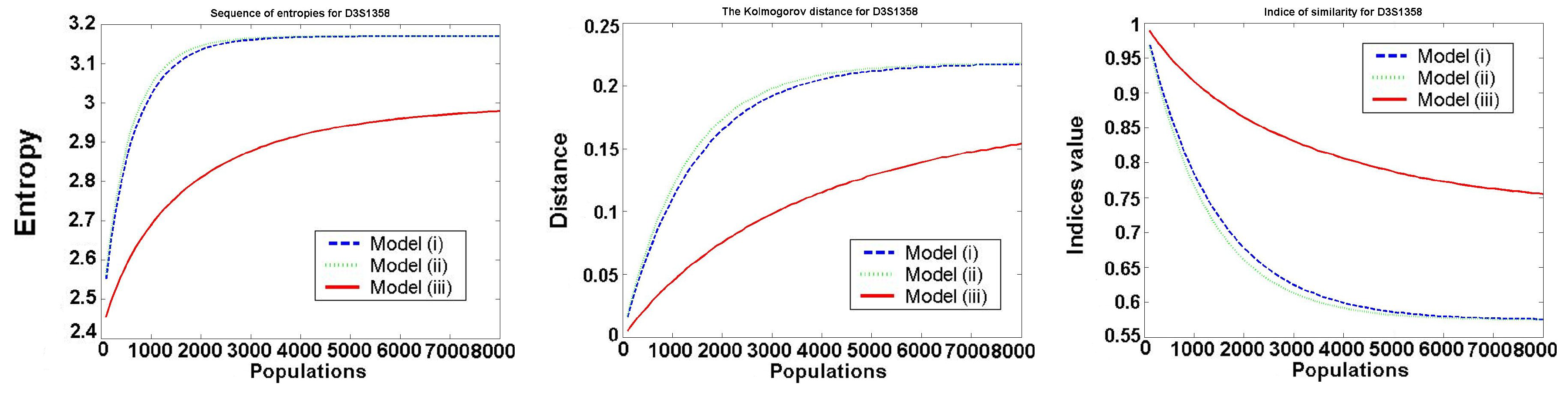
The behavior of the investigated values for one typical locus D3S1358 is presented in the following Figure 2.
We only consider Models 1–3, because in Model 4 all values are constant (it satisfies the Hardy–Weinberg hypothesis). We see that Models 1 and 2 (almost identical in the figures) are worse than Model 3, as the entropy of frequencies increases much faster in Model 1 and Model 2. In all models, the speed of convergence decreases with increasing the number of generations. Thus, the increase is the biggest in the first generation.
For all the investigated values , and for , the best in a mean-square sense is the logarithmic function:
The optimal values for belong to the intervals , , for to , and for to This means that after about 8000 generations, we obtain almost uniformly distributed allele frequencies.
7. Conclusions
- (i)
- The mutation model assumed in the DNA VIEW program is not correct. After a long-time simulation (~8000 generations), this model results in almost uniformly distributed frequencies (the value of entropy in the D3S1358 locus case is over 93% its maximal value, much more than the value observed in human population, and the trend is still growing, however much slower than in earlier generations) of alleles but in reality no such uniform distribution at any locus can be observed. The uniformly distributed allele frequencies give the maximal entropy, but in reality, the entropy at different loci is smaller than the maximal one (between of the maximal entropy in the case of LPL and in the case of Penta E).
- (ii)
- The speed of convergence is directly proportional to the number of allele N and inversely proportional to the difference between the uniform distribution and the distribution of (expressed by ). A statistical analysis gives the formula ( for N and for ). In the case of the Kolmogorov distance and indices of similarity, this dependence is not statistically significant.
- (iii)
- Among the considered models: Models 1, 2, and 3, Model 3 is the best. However, from a viewpoint of the Hardy–Weinberg hypothesis, Model 4 is the best. On the other hand, Models 1 and 4 “change” the observed mutation rate; however, this change is very small. Model 3 is preferred from the viewpoint of genetic observation.
- (iv)
- The choice of model taken for paternity testing has an essential influence in the case of maternal mutation. The only cause why it is hard to detect is that maternal mutations occur rarely. However, if they do, the differences can be enormous, as it was shown in Table 3 ( value 0.0003674 in Model 3 suggests that the man almost sure is not a father while values over 0.9967 in other models contradict this statement). In this case, we may get a different conclusion dependent on the taken mutation model (the defendant is accepted or excluded as a father).
- (v)
Funding
This research received no external funding.
Acknowledgments
The author would like to express his gratitude to the referees for their constructive comments which led to an improved presentation of the paper.
Conflicts of Interest
The author declares no conflict of interest.
References
- Vicard, P.; Dawid, A.P.; Mortera, J.; Lauritzen, S.L. Estimating mutation rates from paternity casework. Forensic Sci. Int. Genet. 2008, 2, 9–18. [Google Scholar] [CrossRef] [PubMed]
- Chakraborty, R.; Stivers, D.; Zhong, Y. Estimation of mutation rates from parentage exclusion data: Applications to STR and VNTR loci. Mutat. Res. 1996, 354, 41–48. [Google Scholar] [CrossRef]
- Kimura, M.; Ohta, T. Stepwise mutation model and distribution of allelic frequencies in a finite population. Proc. Natl. Acad. Sci. USA 1978, 75, 2868–2872. [Google Scholar] [CrossRef] [PubMed] [Green Version]
- Valdes, A.M.; Slatkin, M.; Freimer, N.B. Allele frequencies at microsatellite loci: The stepwise mutation model revisited. Genetics 1993, 133, 737–749. [Google Scholar] [PubMed]
- Caskey, C.T.; Pizzuti, A.; Fu, Y.-H.; Fenwick, R.G., Jr.; Nelson, D.L. Triplet repeat mutations in human disease. Science 1992, 256, 784–789. [Google Scholar] [CrossRef] [PubMed]
- Lai, Y.; Sun, F. The relationship between microsatellite slippage mutation rate and the number of repeat units. Mol. Biol. Evol. 2003, 20, 2123–2131. [Google Scholar] [CrossRef] [PubMed]
- Calabrese, P.; Durrett, R. Dinucleotide repeats in the Drosophila and human genomes have complex, length-dependent mutation processes. Mol. Biol. Evol. 2003, 20, 715–725. [Google Scholar] [CrossRef] [PubMed] [Green Version]
- Whittaker, J.C.; Harbord, R.M.; Boxall, N.; Mackay, I.; Dawson, G.; Sibly, R.M. Likelihood-based estimation of microsatellite mutation rates. Genetics 2003, 164, 781–787. [Google Scholar] [PubMed]
- Crow, J.F. Hardy, Weinberg and language impediments. Genetics 1999, 152, 821–825. [Google Scholar] [PubMed]
- Evett, I.W.; Weir, B.S. Interpreting DNA Evidence: Statistical Genetics for Forensic Scientists, 1st ed.; Sinauer Associates: Sunderland, MA, USA, 1998. [Google Scholar]
- Hartl, D.L.; Jones, E.W. Genetics: Principles and Analysis, 4th ed.; Jones and Bartlett Publishers: Burlington, MA, USA, 1998. [Google Scholar]
- Weir, B.S. Genetic Data Analysis II. Methods for Discrete Population Genetic Data, 2nd ed.; Sinauer Associates: Sunderland, MA, USA, 1996. [Google Scholar]
- Buckleton, J.; Triggs, C.M.; Walsh, S.J. Forensic DNA Evidence Interpretation, 1st ed.; CRC Press: Boca Raton, FL, USA, 2004. [Google Scholar]
- Balakrishnan, N.; Voinov, V.; Nikulin, M.S. Chi-Squared Goodness of Fit Tests with Applications; Academic Press: Cambridge, MA, USA, 2013. [Google Scholar]
- Lemeshow, S.; Hosmer, D.W., Jr. A review of goodness of fit statistics for use in the development of logistic regression models. Am. J. Epidemiol. 1982, 115, 92–106. [Google Scholar] [CrossRef] [PubMed]
- Fisher, R.A. Statistical Methods for Research Workers, 5th ed.; Oliver and Boyd: Edinburgh, UK, 1934. [Google Scholar]
- Raymond, M.; Rousset, F. An exact test for population differentiation. Evolution 1995, 49, 1280–1283. [Google Scholar] [CrossRef] [PubMed]
- Slatkin, M. A correction to the exact test based on the Ewens sampling distribution. Genet. Res. 1996, 68, 259–260. [Google Scholar] [CrossRef] [PubMed] [Green Version]
- Guo, S.W.; Thompson, E.A. Performing the exact test of Hardy–Weinberg proportion for multiple alleles. Biometrics 1992, 48, 361–372. [Google Scholar] [CrossRef] [PubMed]
- Forensic Mathematics. Available online: http://dna-view.com/ (accessed on 26 March 2020).
- Brenner, C. Symbolic kinship program. Genetics 1997, 145, 535–542. [Google Scholar] [PubMed]
- Dawid, A.P.; Mortera, J.; Pascali, V.L. Non-fatherhood or mutation?: A probabilistic approach to parental exclusion in paternity testing. Forensic Sci. Int. 2001, 124, 55–61. [Google Scholar] [CrossRef]
- Butler, J.M. Advanced Topics in Forensic DNA Typing: Interpretation, 1st ed.; Academic Press: Cambridge, MA, USA, 2014. [Google Scholar]
- STRBase SRD 130. Available online: https://strbase.nist.gov/mutation.htm (accessed on 26 March 2020).
- Lütkepohl, H. Handbook of Matrices; Wiley: Chichester, UK, 1996. [Google Scholar]
- Cohn, P.M. Elements of Linear Algebra, 1st ed.; Chapman & Hall/CRC: New York, NY, USA; Washington, DC, USA, 1994. [Google Scholar]
- Kuttler, K. An Introduction to Linear Algebra; Brigham Young University: Provo, UT, USA, 2007. [Google Scholar]
- Goebel, K.; Kirk, W.A. Topics in Metric Fixed Point Theory; Cambridge University Press: Cambridge, UK, 1990. [Google Scholar]
- Vein, R.; Dale, P. Determinants and Their Applications in Mathematical Physics, 1st ed.; Springer: New York, NY, USA, 1999. [Google Scholar]
- Muir, T.; Metzler, W.H. A Treatise on the Theory of Determinants; Dover Publications Inc.: Mineola, NY, USA, 2003. [Google Scholar]
- Aitken, C.G.G. Statistics and the Evaluation of Evidence for Forensic Scientists, 1st ed.; John Wiley & Sons Inc.: Hoboken, NJ, USA, 1995. [Google Scholar]
- Balding, D.J.; Steele, C.D. Weight-of-Evidence for Forensic DNA Profiles, 2nd ed.; John Wiley & Sons: Hoboken, NJ, USA, 2015. [Google Scholar]
Figure 1.
Distribution of at locus D5S818 in the case of maternal mutation. Width shows the probability of obtaining value indicated by the height (axis y on a chart).
Figure 1.
Distribution of at locus D5S818 in the case of maternal mutation. Width shows the probability of obtaining value indicated by the height (axis y on a chart).
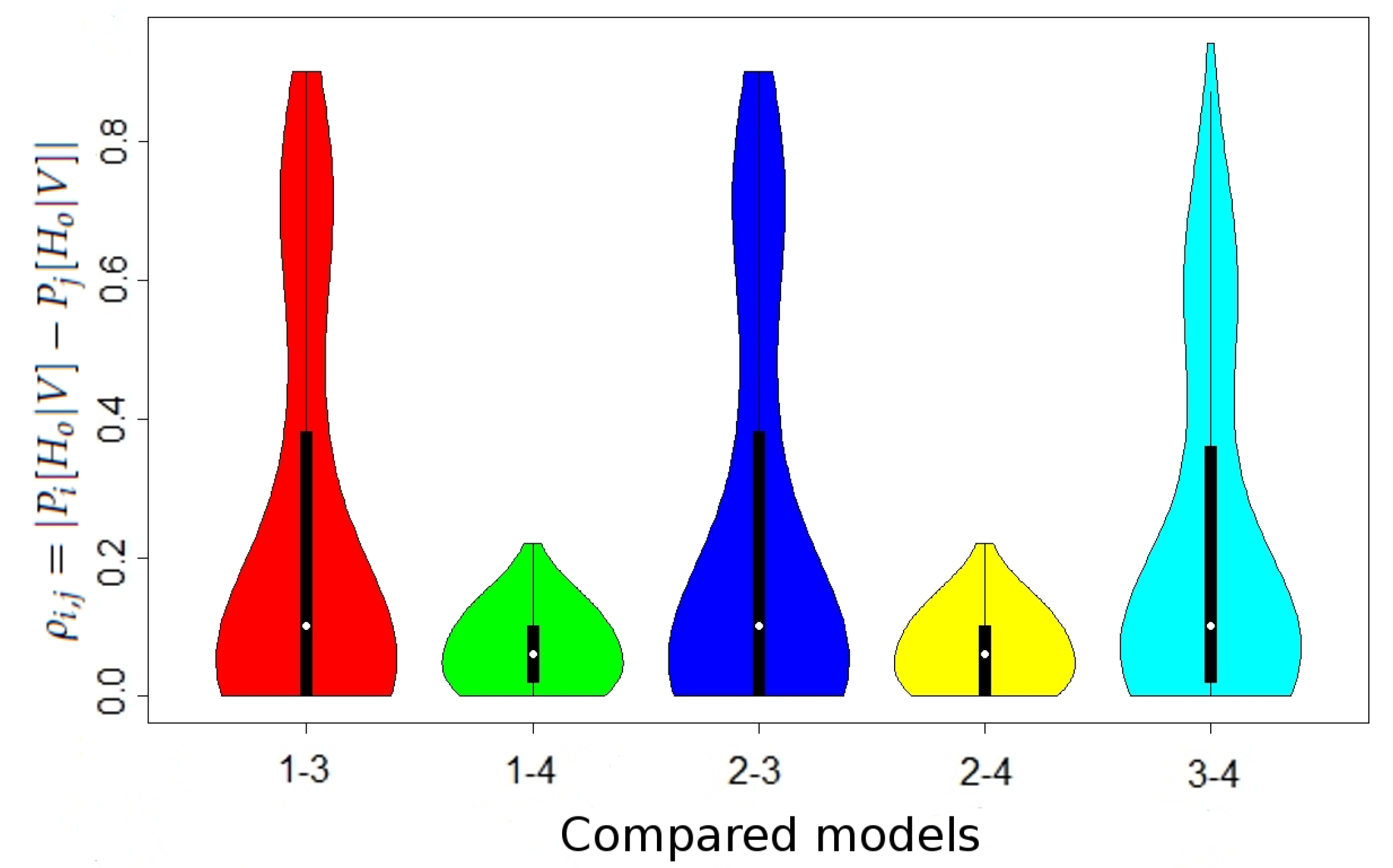
Figure 2.
Investigated values: entropy , Kolmogorov distance , and similarity index in i-th generation and k-th model, for locus D3S1358.
Figure 2.
Investigated values: entropy , Kolmogorov distance , and similarity index in i-th generation and k-th model, for locus D3S1358.


Table 1.
Allele (indicated by the number of gene repetition); frequencies; at the D5S818 locus (cf. [24]).
Table 1.
Allele (indicated by the number of gene repetition); frequencies; at the D5S818 locus (cf. [24]).
| i | i | i | ||||||
|---|---|---|---|---|---|---|---|---|
| 1 | 9 | 7 | 15 | 13 | 20 | |||
| 2 | 10 | 8 | 16 | 14 | 21 | |||
| 3 | 11 | 9 | 17 | 15 | 22 | |||
| 4 | 12 | 10 | 16 | 23 | ||||
| 5 | 13 | 11 | 18 | 17 | 24 | |||
| 6 | 14 | 12 | 19 |
Table 2.
Maximal difference of probability of paternity values between i-th and j-th model () in two cases: with maternal mutation and without it, at the D5S818 locus.
Table 2.
Maximal difference of probability of paternity values between i-th and j-th model () in two cases: with maternal mutation and without it, at the D5S818 locus.
| Maternal Mutation | No Maternal Mutation | |||||
|---|---|---|---|---|---|---|
| Model 2 | Model 3 | Model 4 | Model 2 | Model 3 | Model 4 | |
| Model 1 | 0.00003 | 0.9977 | 0.4237 | 0.00003 | 0.0005 | 0.0003 |
| Model 2 | 0.9977 | 0.4237 | 0.0005 | 0.0003 | ||
| Model 3 | 0.9985 | 0.0006 | ||||
Table 3.
Probability that we achieve DNA profiles V, providing man P is a father of D (), probability that we achieve DNA profiles V, providing P is not a father of D (), and probability that P is a father of D () in the case of at locus D5S818.
Table 3.
Probability that we achieve DNA profiles V, providing man P is a father of D (), probability that we achieve DNA profiles V, providing P is not a father of D (), and probability that P is a father of D () in the case of at locus D5S818.
| Value | Model 1 | Model 2 | Model 3 | Model 4 |
|---|---|---|---|---|
© 2020 by the author. Licensee MDPI, Basel, Switzerland. This article is an open access article distributed under the terms and conditions of the Creative Commons Attribution (CC BY) license (http://creativecommons.org/licenses/by/4.0/).
Share and Cite
MDPI and ACS Style
Krajka, T. Mutation Rate Model Used in the DNA VIEW Program. Appl. Sci. 2020, 10, 3585. https://doi.org/10.3390/app10103585
AMA Style
Krajka T. Mutation Rate Model Used in the DNA VIEW Program. Applied Sciences. 2020; 10(10):3585. https://doi.org/10.3390/app10103585
Chicago/Turabian StyleKrajka, Tomasz. 2020. "Mutation Rate Model Used in the DNA VIEW Program" Applied Sciences 10, no. 10: 3585. https://doi.org/10.3390/app10103585
Note that from the first issue of 2016, this journal uses article numbers instead of page numbers. See further details here.