Rapid Restoration Techniques for Software-Defined Networks


1
School of Electrical and Electronic Engineering, Technological University Dublin, Dublin D08 NF82, Ireland
2
School of Computing, University of Portsmouth, Portsmouth PO1 3HE, UK
*
Author to whom correspondence should be addressed.
Appl. Sci. 2020, 10(10), 3411; https://doi.org/10.3390/app10103411
Submission received: 9 April 2020
/
Revised: 6 May 2020
/
Accepted: 12 May 2020
/
Published: 14 May 2020
(This article belongs to the Section Electrical, Electronics and Communications Engineering)
Abstract
:There is increasing demand in modern day business applications for communication networks to be robust and reliable due to the complexity and critical nature of such applications. As such, data delivery is expected to be reliable and secure even in the harshest of environments. Software-Defined Networking (SDN) is gaining traction as a promising approach for designing network architectures which are robust and flexible. One reason for this is that separating the data plane from the control plane, increases the controller’s ability to configure the network rapidly. When network failure events occur, the network manager may trade-off the optimality of the achieved network reconfiguration with the responsivenss of the reconfiguration process. Responsiveness may be favoured when the network resources are under stress and the failure rate is high. We contribute SDN recovery methods that leverage information about the structure of the network to expedite network restoration when a link failure occurs. They operate by detecting community-like structures in the network topology and then they find alternative paths which have low operation and installation costs using this information. Extensive simulations are conducted to evaluate the proposed SDN recovery methods using open-source simulation tools. They provide evidence that the proposed approaches lead to performance gains when an alternative path is required among a set of candidate paths.

1. Introduction
Software-Defined Networking (SDN) has emerged as a promising approach for defining network architectures that are highly adaptable and robust. Realising the demands of the future Internet is becoming more attainable. SDN was conceived at Stanford University as a clean slate approach [1] to redesign the network architecture and to facilitate the evolution of the future Internet. In a SDN, the data and control planes are physically decoupled which results in a network consisting of—(1) a centralised controller that maintains a global view of the network state, and (2) simple forwarding elements whose packet forwarding behaviour is dictated by the controller. Due to its programmable interfaces, SDN offers new opportunities to implement new routing strategies, customised traffic engineering, dynamic allocation of network resources and many other programmable functionalities. In other words, SDN opens the door to accommodate network innovations. So far, some leading companies such as Google, Microsoft and Huawei have employed SDNs in their data centers and in the near future SDN is expected to play a part in 5G [2]. As with any new innovation, SDN faces several challenges such as those related to the management of network failures and the reconfiguration of the network by updating the network architecture [3]. Network elements, such as forwarding devices and links, are susceptible to failure incidents. As a consequence, network facilities like routing will be harmed. Recovery from failure can be achieved either proactively, which is also called protection, or reactively, which is also called restoration [4]. In protection, the alternative solution is pre-planned and reserved before a failure occurs. However, in restoration, the solution is not pre-planned and needs to be calculated dynamically (on demand) when a failure occurs.
On one hand, protection mechanisms are expensive [5] as they require two paths to be installed for each flow and this could overwhelm critical network resources such as switch Ternary Content Addressable Memory (TCAM). Moreover, the backup path may not be available when it is needed. The backup path could fail earlier than the primary one. On the other hand, restoration mechanisms are time consuming as the network controller will first need to calculate an alternative path and then install the flow entries (i.e., forwarding rules) in the relevant switches. The time required to reconfigure the network includes two factors: (1) the time to calculate a new path and (2) to update the switches on the new path. In this paper, we focus on restoration techniques. Our main aim is to accelerate network recovery from a single link failure in large scale networks by reducing the duration of the network updating process, speeding up network restoration. Our SDN recovery methods exploit the inherent structured nature of networks to find a quick solution when a link failure is detected.
This paper is organised as follows—in Section 2, various SDN fault management techniques are presented and discussed. In Section 3, we introduce our network model along with the proposed methods. We then illustrate the proposed framework to tackle link failures using the proposed methods in Section 4. Simulation and experimental results are presented in Section 5 and we conclude by outlining our future work. Finally, the summary of this paper is provided in Section 6.
2. Related Work
Link failures, which last for different time periods and have different causes, take place in everyday network operation [6]. For example, an evaluation of the susceptibility to link failure of business critical processes in a data-centre, which manages 75% of Europe’s flight bookings, was undertaken in Reference [7]. A crucial finding was that susceptibility to link failure was intrinsically linked to the network topology. Although much research in the literature has been dedicated to considering this issue from different perspectives (analysis, characterization, evaluation and recovery), the new network architecture of SDN requires more investigation. We discuss some recent works which are related to our proposed SDN recovery approach.
In References [8,9], the authors discussed the possibility of achieving carrier-grade reliability. This was defined as having the ability to recover from failures within 50 s. These approaches were based on following the loss of signal to ascertain if there were changes in the network topology such as failures. When a notification about link failure was received by the controller, the controller identified the affected paths, it calculated alternative paths, and finally, it sent the appropriate flow modification instructions to the switches. Evaluations were carried out by both studies using small-scale networks, which consisted of 6 and 14 nodes. These studies demonstrated that recovery times of less than 50 s could be achieved, satisfying the targets set for evaluating carrier-grade reliability. However, the authors conceded that the restoration time also depended on the number of flows (i.e., rules) that needed to be modified in the affected path, therefore, the recovery time was far from the carrier-grade threshold in some of their experiments. It is a significant challenge to meet the carrier-grade reliability requirement posed by large-scale networks. The authors did not take into account the correlation between the path length and the recovery speed. In addition, they did not attempt to reduce the operations required to set-up the backup paths. The authors of Reference [10] proposed a restoration scheme called Automatic Failure Recovery for OpenFlow (AFRO), which worked in two phases, namely, record mode and recovery mode. In record mode, AFRO recorded all the controller-switch activity (e.g., PACKET-IN and FLOW-MOD) in order to create a clean state copy of the network when no failure was experienced. When a failure occurred, AFRO switched to the recovery mode. This was followed by generating a new instance of the controller (a shadow controller). This copy was a copy of the original state but it excluded the failed elements. Then, all the recorded events were replicated for the sake of installing the different rule-set between the original and shadow copies. The authors produced a prototype of AFRO, however, the study lacked any simulation results and/or measurements to show the effectiveness of AFRO. Moreover, the process of switching from record mode to the recovery mode required time, which had the potential to cause service disruption.
The network resilience achieved by the approach in Reference [11] was given as the reason for the convergence delay experienced after failure events. Speed of fail-over was attributed to two parameters: (1) the distance between the controller and the site of failure; and (2) the length of the alternative path that was computed and then installed by the controller. The authors increased the speed of failure recovery by deploying multiple centralized controllers to enable the dynamic computation of end-to-end paths; this innovation also had the benefit of increasing the resilience and the scalability of the solution. This work did not take into account the time required for the recovery process. Instead failure detection was accelerated.
CORONET was introduced in Reference [12] to achieve fast network recovery from multiple data plane link failures in SDNs. CORONET was based on slicing the network into VLANs so that the ports of physical switches were mapped to different VLAN IDs. A route planning module computed multiple link-disjoint paths using Dijkstra’s algorithm [13]. When one or more link failures occurred the controller used a set of pre-computed paths to assign an alternative route to address the link failure(s). A secondary benefit of CORONET was that calculated disjoint paths could be used to perform load balancing. Dynamic load balancing was achieved by using different paths in a round-robin manner based on monitoring reports from a traffic monitoring module which performed traffic analysis. The system was prototyped using the NOX controller and it is compatible with the standard OpenFlow protocol.
In Reference [14], the authors proposed HiQoS, a SDN-based solution that finds multiple paths between the source and destination nodes to guarantee certain QoS constraints such as bandwidth, delay and throughput. HiQoS used a modified Dijkstra algorithm to learn the multiple paths required to meet the QoS requirements. Not only could the QoS be guaranteed with HiQoS, but also a fast failure recovery could be achieved. This is because when a link failed it caused a truncation or interruption in some paths. The controller then directly selected a working path from the already computed ones. The authors compared the performance of HiQoS, which supports multiple paths, against MiQoS, which is a single path solution, and experiments showed that HiQoS outperformed the MiQoS in terms of performance and resilience to failure. Unfortunately, the authors did not provide a deep explanation of how the proposed method accelerated the restoration and reduced the recovery time.
The authors introduced the Smart Routing framework for SDNs in Reference [15], which allowed the network controller to receive forewarning messages about failures and therefore to reconfigure the potential paths before failure incidents occurred. However, this technique required historical data. This data may not be available in scenarios that do not require pre-existing infrastructure, for example, ad-hoc networks. In this scenario it is difficult to motivate the use of Smart Routing. Several studies like those in References [16,17,18] have addressed the problem of optimising failure restoration as an Integer Linear Program (ILP). However ILP-based approaches may be slow to converge in large-scale networks [19]. In practice, achieving fast recovery would require faster solvers. In References [20,21], the authors considered the problem of path-switching latency in heterogeneous networks, where nodes had different specifications. The proposed method selected alternative paths based on the switches which had the shortest processing time. However, the proposed approach was tested on a small-scale network. Also, the study did not discuss the cost associated with the improvements achieved by the method.
Notwithstanding our previous discussion on multi-controller solutions, SDN is traditionally a centralised networking architecture. One of the main responsibilities of its central point, the controller, is to maintain the routing tables of all the nodes that reside on its domain. Network forwarding elements potentially operate in harsh environments, such as unreliable wireless sensor networks, where failure rates are high, causing frequent changes in the network topology [22]. Similarly, the forwarding elements might operate in dynamic environments where the installed rules have to be updated frequently, for example, every 1.5 to 5 s [23]. In such a case, the re-routing activities need to take place quickly in order to cope with the frequent changes. In other words, searching for optimal solutions might be costly in terms of installing and updating rules considering that the lifespan for such rules may be short. Although the amount of research conducted in the area of SDN fault management is growing, most of the contributions so far have focused on replacing the affected paths with new optimal ones. In this paper, the main goal is to accelerate the set-up of alternative paths in order to facilitate fast switch-over.
We can summarise the contributions of this paper as follows.
- A Community Detection (CD) approach is proposed where the network topology is divided into a number of communities, which we denote N. The aim is to find the alternative paths within a sub-graph (i.e., community) rather than the whole graph.
- A Path Anatomy (PA) approach is proposed in which the affected path is tackled partially rather than from end-to-end.
Our contributions enhance the reactiveness of SDN fault management. We achieve this reactivity by reducing the number of rules that must be replaced. This, in turn, lowers the number of nodes that need to be updated and therefore, speeds-up the switch-over.
3. Proposed Path Recovery Methods
3.1. Network Model
We start by outlining the notation used in the paper. Due to the nature of communication between appliances, an undirected graph is widely used to model the status of computer networks [24]. A graph, G, is defined as, , where V represents the finite set of nodes (i.e., routers) in G, and E represents the finite set of bidirectional edges (i.e., links) in G that connect the nodes to one another. The set of all edges in a graph is a 2-element subset of nodes, . A path P is a sequence of nodes . Pairs of nodes in a path are members of the edge-set, . Here, and are called the source and destination nodes of P, respectively. A path, P, is simple if it contains no loops. The length of P is the sum of the weights (costs) of its constituent edges; that is . The shortest path from to is the path with the shortest length in the set of all available paths between and , . We use the hop count to measure the distance between and , which means that all edges have equal weighting, . In this paper, Dijkstra’s algorithm [13] is used to find the paths with the minimum hop count.
3.2. Community Detection-Based Approach
Community Detection (CD) considers that groups of nodes that share common properties can be represented as communities [25]. Here each community is defined as a subgraph whose nodes are densely connected, but sparsely connected with the rest of the network [26]. Many algorithms have been proposed to discover community structures in networks such as the Louvain algorithm and the Girvan and Newman algorithm [27]. Figure 1 shows a synthetic network on the LHS and a representation of the network on the RHS which consists of three non-overlapping communities which are detected using a community detection algorithm. Each community only has two inter-community links whereas nodes within communities are densely connected.
Community detection has been utilised to resolve various kinds of network-related problems such as routing and data forwarding [28,29]. We use the concept of a community as an approach to improve the speed that an SDN is restored by accelerating the process of failure recovery. By dividing the network graph G into N communities, we make the assumption that when a link failure event occurs, only one community will suffer from that particular failure. If this is the case, the other communities will continue working properly, since no failure is experienced in their domain. The assumption that only one community is affected is reasonable in a large proportion of the cases of link failure. This assertion is true because the criteria that we use to partition the network into communities is link density, and thus, as the density of edges between nodes in the community is higher than the density of inter-community edges, and if the link failure probability is uniform, link failure events are more likely to be confined within one community. It is worth bearing in mind that link failure probabilities will not in general be uniform. In this case the link failure probability may also be incorporated into the community detection process to address this problem. We assume that the link failure distribution is uniform. At the moment of link failure, only the community that includes the affected link will be considered in order to find a path recovery solution. The advantage of our approach is that instead of searching for an alternative path from end-to-end within an entire graph, G, we only consider the problem within a single community.
3.2.1. CD Model
The number of communities extracted by a community detection algorithm depends on the network topology structure and the parametrization of the community detection algorithm. We define the set of communities which partition the network graph as , where , , and where N is the number of communities. Each individual community consists of a subset of the graph node-set and the graph edge-set:
A path, P, between a source and destination, which traverses K communities, starting at the source router, , ending at the destination router, , and passing through the intermediate nodes, and , for is
The set of learned communities is mutually exclusive. The intersection of the node-set of community and community is the empty set. The intersection of the edge-sets of these two communities is also the empty set,
A failed link, a 2-router sub-path, , in P is
This definition of considers only those cases where failed links are always of an intra-community type. In other words, we assume that consecutive routers in a path, for example and , must be in the same community,
The set of all Dijkstra-based solutions for a given network topology is denoted
where represents the set of all possible paths between any two particular nodes, that is, and . When we apply Dijkstra’s algorithm to G, we denote the solution , and when it is applied to a community c the solution is denoted . The network’s diameter quantifies the length of the shortest path between the two most distant nodes. The shortest path between the two most distance nodes is called the longest-shortest path. The function , takes a set of paths, , as its argument, to determine the longest-shortest path.
If there is more than one longest-shortest paths in , we pick one randomly. The case of the longest-shortest path is of particular interest. It represents the worst case scenario in terms of the number of rules that need to be updated by the controller as a result of the need for modification.
3.2.2. CD Example
A schematic example is provided to clarify the strategy of our community detection-based approach. The European Reference Network (ERnet) [30] topology, which has 37 nodes and 57 edges is used as a case study. We use different coloured regions in Figure 2 to illustrate the non-overlapped communities, which were learned by the Girvan and Newman algorithm [31]. Consider the path between Dublin and Sofia. The least cost path between these two nodes is through the route:
Dublin–London–Paris–Lyon–Marseilles–Rome–Zagreb–Belgrade–Sofia
Now, let us assume that the link Paris–Lyon fails. After discovering the change in the network topology due to the failure, the network controller is required to calculate a new path and to update the network. As the selected path passes through 4 communities, yellow, orange, red and blue, this means that only one community needs to be considered in order to find an alternative path. In this case, only the affected segment of the path, which passes through the orange community, will be involved in the process of rule replacement and updating. To update the rules, the proposed solution finds the shortest path between the two routers on both sides of the failed link, that is, between Paris and Lyon. Therefore, the controller only needs to replace and update four routers of the sub-path (Paris–Strasbourg–Zurich–Lyon). The rest of the nodes, which are distributed over the other communities, remain in the same configuration and order.
3.3. Path Anatomy-Based Approach
In Section 2, we discussed techniques that pre-computed backup disjoint paths to deal with failure events. The controller first removed the entire set of old flow entries on the affected path and then installed the required rules for the alternative path. This process is time-consuming when the length of the affected path is long. A network Path Anatomy (PA) is a potential solution to this problem. A network PA partitions a path instead of partitioning the graph. An illustration of how this works for a path from point to point is depicted in Figure 3.
This sequence of adjacent routers has some middle router(s), which are denoted . The path P can be divided into two segments. Finding a new path from to in order to overcome the failure may not be an effective solution. This is because the cost of rule replacement and updates can be high. A PA overcomes this problem. We outline two schemes to implement a PA-based approach. The first one uses the middle routers of P to consider two parts (i.e., sub-paths), one of them is running and the other is not (due to a failure for example). This means that one segment of the affected path can still be utilised as is and the operation cost to update that segment is zero. In the second scheme, instead of replacing the faulty segment of the path with a new sub-path, the search space for an alternative path is reduced to be only between the two nodes surrounding the failed link. The second approach finds an alternative path between the two nodes of the failed link. Searching for an alternative sub-path rather than an end-to-end path means that the proposed solution makes the search space smaller and the makes the rule update time shorter. We continue by describing these schemes.
3.3.1. PA Model
We define the function, , which takes a path P as its argument, to determine the middle point of the path P. We also introduce the function , which operates on a sequence of nodes and returns the next node in the sequence relative to a second arugment which is a node in the sequence, . For example,
for any When the next node is not a member of the input sequence of nodes the output is the empty set. For example,
Similarly, the function , which also operates on the sequence and takes a reference node as its second input, computes the previous node relative to the reference node, .
for any . The result achieved is the empty set, when the reference node passed to leads to a solution which is not in the sequence argument, for example,
The function is now defined as
The output of is called M for simplicity. The middle point represents a set consisting of either the two middle nodes in a path, in the case where the length of the path is even, or a single middle node, when the length of the path is odd. A path of length 2 has an empty middle point set. Using the function , we introduce functions that determine the first and second part sets of a path P relative to router . The function denotes the first part of a path, and denotes the second part of a path.
Both and return the empty set. Using these functions, we define a failed link (i.e., a 2-node sub-path), , in a path P as a case of one of two scenarios, in relation to some node in the path P:
The above definition expresses failures in two cases, both with respect to a node, . The first failure is in a link with a node following , whereas the second is in a link with a node preceding .
3.3.2. PA Example
A schematic example is provided to clarify the strategy used by the path anatomy approach. We re-use the ERnet topology in Figure 2, however, the coloured layer is discarded. Consider the path between Dublin and Sofia. The least cost path between these two nodes is through the route:
Dublin–Glasgow–Amsterdam–Hamburg–Berlin–Prague–Budapest–Belgrade–Sofia
As this path has 8 hops and is of length 9, its middle point is Berlin. Let us assume that the link Hamburg–Berlin fails. The recovery procedure reacts to the failure by asigning the two affected nodes to the failed link set, . The controller then treats the failure using the first or the second PA scheme. In the case of the first scheme, the retrieved alternative sub-path will be:
Note that the change affects only part of the original path, its first half (between Dublin and Berlin), where the failure has occurred. However, using the second scheme, the alternative sub-path returned will instead be:
In the second case, the solution is specific to the two nodes between which the failed link lies, Hamburg and Berlin.
Dublin–Glasgow–Amsterdam–Hamburg–Frankfurt–Munich–Berlin
Hamburg–Frankfurt–Munich–Berlin
4. Path Recovery Framework and Algorithms
Four path recovery algorithms are described. Algorithm 1 does not use community structure to determine the best recovery path. Algorithm 2 forms the recovery path by considering the community in which the failed link lies. Algorithms 3 and 4 use the PA approach to determine recovery paths. The implementation code of the current framework is made available on the GitHub platform (https://github.com/Ali00/SDN-Restoration). We start by introducing our system framework, which makes components available to the recovery algorithms. Then we describe the 4 recovery algorithms. Figure 4 illustrates the main components of our framework. The two components, that is, Community Detection and Path Anatomy, are the main contributions of this framework. We describe the components used in this framework below.
4.1. SDN Controller
The SDN controller represents the network’s brain. It is where the intelligence and decision making is performed by the framework. We use the POX controller as it facilitates fast prototyping [32]. The standard OpenFlow protocol [33] is used as a southbound API for establishing the communication between the data and control planes, whereas the set of POX APIs is used on the northbound interface for developing various network control applications.
4.2. Topology Parser
The topology parser is responsible for fetching the underlying network topology characteristics and building a topological view with the aid of the POX openflow.discovery [34]. In order to represent the network topology as a graph, G, we utilised the NetworkX [35] tool in order to be able to manipulate and simplify the underlying topology.
4.3. Global Recovery Scheme
The set of steps that the SDN controller takes after detecting a data plane link failure are determined by the global recovery scheme component. When an OpenFlow controller reports a failure status, the failed path is first identified before the SDN controller installs a backup path that detours the disrupted flows and achieves the recovery of the network. These steps are described as follows. First, a clear command is sent to all of the involved routers that belong to the failed path. Then, an alternative path is computed from the source router to the destination router (lines 1-2 of Algorithm 1). Finally, the computed flow entries of the alternative path are forwarded to the relevant routers. This end-to-end algorithm is included to serve as a useful and reasonable benchmark algorithm to compare with our contribution. It does not exploit community structure to ensure rapid recovery.
| Algorithm 1: Find the shortest path with Dijkstra from End-to-End based on Graph G |
| On Normal: |
| On Failure: |
4.4. Community Detection
The community detection component is composed of a community finder sub-component and a community detection-based fault handling sub-component which form crucial components of Algorithm 2.
| Algorithm 2: Find the shortest path with Dijkstra on the basis of either G or the affected community () |
 |
4.4.1. Community Finder
The community finder creates a virtual partition of the network topology graph, G, into C (i.e., sub-graphs) using the community detection algorithm, Girvan and Newman [31]. The communities may have different sizes. We desire that the graph, obtained by the topology parser, is partitioned so that the members of communities that are formed as a result of the partition of the network are densely connected. This dense interconnection property is one of the main features of the Girvan and Newman algorithm. By using this algorithm, the dense inter-connectivity in each community provides multiple alternative paths that can be utilised when failure events occur. We rely on the implementation of the Girvan and Newman algorithm in Reference igraph [36] to partition G.
4.4.2. CD-Based Fault Handling
Based on the global view of the underlying topology that is constructed from the topology parser, the community detection-based fault handling module is responsible for determining the demand paths that carry the flows across the network. Invocation of the route finder occurs in two situations: (1) when a new packet arrives on the network and the calculation of a new path is required; (2) when a failure occurs and it is necessary to recalculate the path for an existing path. Two algorithms are developed to obtain the shortest path based on Dijkstra’s algorithm to meet the needs of these two use-cases. In our approach, the community-based algorithm tackles failures based on the affected community, for example, , instead of recalculating paths based on the the whole graph G (cf. lines 2–3 of Algorithm 2). Currently, Algorithm 2 takes advantage of the community based approach when a failure occurs within a community and it falls back on the Global recovery approach when the failure occurs on links between communities, as a future development the framework will be extended to include the inter-link failure among the set of communities. The worst case computational complexity of Dijkstra’s algorithm bounds the computational complexity of Algorithms 1 and 2. Using a Fibonnaci heap the worst case computational complexity for the entire graph G is . An appealing property of our approach is that when community detection is performed the node and edge-sets within the communities are much smaller than the node and edge sets for the entire graph. The worst-case computational complexity in the case of a failure is much lower in Algorithm 2 as Dijkstra’s algorithm is only run on the sub-graph contained within a community. In comparison, when Algorithm 1 is used in the case of a failure, the entire graph, G, is considered in the Dijkstra update step. This is because Algorithm 2 performs Dijkstra’s algorithm based on the affected community in order to learn an alternative path rather than on whole the graph, as in Algorithm 1. The relationship between the computational complexity saving for the worst-case scenario for the entire graph and a community is expressed as:
As the number of communities detected in the graph increases, the left-hand-side of this inequality dominates. On the other hand, if too many communities are detected the range of alternative paths available to Algorithm 2, to determine an alternative path is restricted. In the worst it may not be possible to determine a better path within the community.
4.5. Path Anatomy
The path anatomy component is comprised of two path anatomy-based fault handling schemes which are described in Algorithms 3 and 4.
4.5.1. PA-Based Fault Handling (Scheme 1)
Scheme 1 is based on the concept of the middle router and given in the listings in Algorithm 3. The set of middle points of a path P is denoted as . Relative to M and assuming that a path deals with one link failure at a time, this failure can be located in either the or sides of the path. Link failure can occur on both sides of the point M in Figure 3. However, in this paper, we do not consider the case of simultaneous failure in both sides of the path. Therefore, we assume that failures do not occur instantaneously, and thus, when the first failure occurs it is dealt with, and then when the second failure occurs it is dealt with. Extending the definition of to include multi-failure scenarios so that multiple failure can be treated in batch without significantly increasing the computational complexity, will be considered in future work. In our current approach, the controller is notified about the failed link, and routers on both sides of the failed link are added to the failure set . When the failure set is the null set, , Algorithm 3 detects the position of the failed link; whether it is above or below M. Once this is done, the affected side is replaced by a new sub-path, which is typically from either to M or from M to . As a result, a minimum of half of the flow entries do not need to be replaced.
| Algorithm 3: Find the Shortest Path with Dijkstra’s from End-to-Mid in a Graph G |
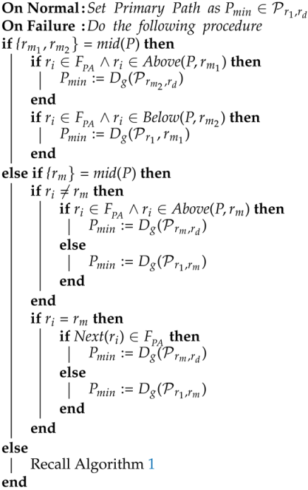 |
4.5.2. PA-Based Fault Handling (Scheme 2)
This scheme focuses on reducing the number of replaced segments within the faulty path and is given in the listings in Algorithm 4. It is a special optimised case of scheme 1, which attempts to find a loop-free shortest path between the routers on both sides of the failed link, that is, between the two nodes of . This is useful because not replacing a full section of a path releases some of the non-affected rules. Only two rules need to be removed. They are located in the routers of the failure set. Thus, the algorithm guarantees that the minimum number of rule modifications are made. The total number of added rules usually depends on the network topology structure.
| Algorithm 4: Find the Shortest Path with Dijkstra’s from Node-to-Node in a Graph G |
 |
5. Experimental Evaluation
Three parameters are important when evaluating the cost of selecting alternative paths using the recovery schemes presented in Section 4. We evaluate our approaches for achieving rapid restoration of SDNs in the event of link failures and compare them with the global approach using the headings: (1) length, (2) operation and (3) latency. The length of a proposed solution indicates the number of hops associated with the new path found by the recovery solution in the event of a link failure. A solution’s operation cost measures the required number of operations to set-up the new path. Typical operations include addition, removal and modification of flow entries. The latency measure indicates the time required to install the alternative path. To evaluate the algorithms with respect to these parameters for different scenarios we constructed networks with different diameters and densities and also numbers of nodes and edges. Table 1 summarizes the statistics of the networks considered. We continue by describing the environment used to evaluate path recovery approaches. Simulation results are then presented in order to compare the efficiency of the proposed approaches with the global approach.
5.1. Real-World and Simulated Network Topologies
Three real-world network topologies were used in order to evaluate the different recovery algorithms—ERnet [30], Germany50 [37] and NR from the Network Repository [38]. They are illustrated in Figure 5 and their characteristics are summarised in Table 1 in terms of the node and link count, the diameter of these networks and their densities.
We used the Internet topology generator Brite [39] to generate additional topologies. Using Brite we generated random graphs using the Waxman [40] algorithm. Waxman’s approach uses the idea that in real networks physically longer links are often more costly to construct, therefore they are less likely to exist. The function is the Euclidean distance between u and v. The constant, , represents the maximum distance between any two nodes. Waxman’s model links () with a probability, , as a function of the negative exponential of the distance between them,
The parameter , which must be positive, tunes the sensitivity to distance of the negative exponential. The scaling term is chosen to satisfy the constraints . The number of links between nodes is determined by the value of . The edge distance typically increases when the value of is incremented. Based on Waxman’s model, we used Brite to generate three synthetic large scale network topologies, namely Brite1, Brite2 and Brite3.
5.2. Performance Evaluation
We considered the performance of recovery algorithms when link failures occurred on a range of different path lengths. In order to be able to draw conclusions from results for network topologies which had different sizes we normalised the path lengths. The length of the longest shortest path is identified for each experimental topology in Table 1 in the column entitled diameter. Each admissible path in was classified based on its normalized length, for example, its length-percentage. Paths were categorised as having a length which varied from 20 to 100 percent of the longest shortest path length in the topology. This approach allowed us examine different categories of paths for different networks sizes. Having established a way to compare results across different networks we now outline the process of our evaluation in Procedure 1. Lines 2–4 of the below evaluation procedure describe how link failures are caused and resolved. Line 4 describes how path recovery is achieved using different approaches. Lines 5–7 describe how metrics are computed in order to evaluate each of the recovery approaches.
| Procedure 1: Process of Evaluation | |
| 1: Select paths with different lengths | ▷ ranging from 20–100% of the LS length |
| 2: For each selected path, choose a random link | |
| 3: Remove the randomly chosen link | |
| 4: Find the alternative path | ▷calculated with Algorithms 1–4 |
| 5: Measure the new path length cost | ▷hop count |
| 6: Measure the new path operation cost | ▷ added and removed flow entries |
| 7: Measure the new path latency cost | ▷installation time |
The proposed framework was implemented and evaluated by using the container-based emulator, Mininet [41]. As evidenced in the survey in Reference [42], Mininet is a widely used emulation system for emulating/simulating network architecture with various experimental scenarios as well as to evaluate and prototype SDN protocols and applications.The experiments in this paper were designed based on the out-of-band mode, where the data traffic was conveyed over a separated medium of the control traffic. Finally, in the emulation environment, we employed two servers; one acted as the OpenFlow controller and the other simulated the network topology. For each server, we used Ubuntu v.14.04 LTS with Intel Core-i5 CPU and 8 GB RAM.
5.2.1. Path Length Cost
We evaluated the average path cost, which was measured in terms of the hop count of the alternative path found by the recovery solutions, Algorithms 1–4. This trial was run for link failures on paths of normalized length which ranged from 20% to 100% in steps of 10%. Figure 6 shows the average path cost obtained by each algorithm as a function of the percentage path length for all the simulated topologies. These values are rounded and summarized in Table 2 for convenience in order to draw conclusions across topologies. The best solution has the lowest average path cost.
The max and min values are also shown. The dotted bar represents the optimal path cost determined by Dijkstra’s algorithm. This path was obtained prior to link failure occurring and served as our benchmark even though it was not feasible after a link failure. We called this solution Before Failure (BF). The new approaches in this paper were compared to this unfeasible, optimal solution in order to make statements about the near-optimality of the learned alternative paths. In the event of a failure it was not possible for an algorithm to perform better than the BF failure approach; in the best case, the achieved solution had a similar path length cost. The proposed approaches attempted to reduce the operation cost, but this came at the price of increasing the path cost. On average, the path cost achieved by Algorithm 1 was close to the optimal path cost, that is, BF. In the worst case, the relative increase in the cost was low and never exceeded 5.2%. Algorithms 3 and 4 achieved an average path cost that was close to the one achieved by Algorithm 1. In the worst case scenario, the relative increase in the cost was not significant, and never exceeded 11.2%. Algorithm 2 provided approximately the same performance as Algorithms 3 and 4. On average, the relative increase in the path cost never exceeded 11.2% in all of the experimental topologies except for Brite2. In Brite2 topology, the relative increase in the path cost was 50% in some cases. Further investigation was warranted to better understand the behaviour of Algorithm 2. To this end, an additional calculation was conducted in which the completion rate and modularity of each topology was measured.
The completion rate is a binary score that measures the success and failure rates of path recovery algorithms. Modularity is defined as an indicator to measure the strength of partitioning the network graph into a number of communities. The modularity score measures the quality of graph partitions after the application of the community detection algorithm. The higher the modularity value the better the decomposition of network. The modularity of each network was measured using the approach in Reference [43]. To measure the completion rates, the success rate was defined as the percentage of successful events compared to the total number of paths in whose length fell within the predefined range (i.e., 20–100). The failure rate was defined as the percentage of fail events compared to the total number of paths in that satisfied the same range of length condition. The flowchart in Figure 7 illustrates how both successes and failures were calculated. All admissible paths that satisfied the length condition were considered in this evaluation. Starting with the first path, a random link failure was generated. After that, the state of the alternative path was checked by applying the Algorithm_x function, where . Setting gave rise to Algorithm 2 being used. Every time Algorithm_x succeeded in obtaining a solution, the success variable was incremented, otherwise the failure variable was incremented instead. Then the broken edge, which was randomly selected in the earlier stage, was re-attached to the network graph G and the process continued to the next path until the end was reached. Table 3 lists the completion rates, intra-links density and modularity along with the number of communities in each network. Based on the results in Table 3, the completion rates were affected by the modularity and links density. The higher the modularity and links density values the better the success rate. Therefore, the Brite2 topology had the lowest modularity and links density values out of all the topologies. Hence, it had the highest failure rate and lowest success rate compared to the others. It is worth mentioning that the success rate for the rest of the algorithms (i.e., Algorithms 3 and 4) was 100%. Given that the success rate of Algorithm 2 was not 100%, this suggested that the algorithm was unable to discover an alternative path all the time. In some cases, the min and max cost were equal to the average cost.
5.2.2. Path Operation Cost
The performance of the proposed approaches was studied with respect to the operation cost, that is, the number of added and removed rules. Paths with different lengths were selected in the manner described in Section 5.2.1. Figure 8 shows the the average operation cost achieved by Algorithms 1–4 versus the percentage of path length for all the simulated topologies. The cost here implies the number of operations required to establish the obtained paths. The max and min values were also reported. The dotted bar represents the required rules to install the optimal path, which serves as the case before failure (i.e., BF) scenario. In most cases, Algorithms 2–4 outperformed Algorithm 1 in terms of the average operation cost. This is due to the fact that the proposed approaches obtained alternative paths by achieving the restoration across a path segment rather than the entire path.
As a consequence the required number of rule updates was reduced. Compared to the operation cost of the optimal path before failure scenarios (i.e., BF), the average operation cost of Algorithm 1 was relatively high and usually depended on the length. The relative increase of the operation cost never exceeded 80% for short paths and 66.6% for long paths. However, compared to the average operation cost obtained by Algorithm 1, the average operation costs achieved by Algorithms 2–4 were lower. The relative decrease in the path operation cost was significant (using Algorithms 2–4) as illustrated in Table 4. We observed that the operation cost was inversely proportional to the path length. The longer the path the lower the operation cost and therefore the higher the reduction rate. In general, Algorithms 2–4 performed better than Algorithm 1 in terms of the operation cost of alternative paths. However, Algorithms 2–4 only failed in 5 out of 162 cases. This is highlighted in bold in Table 4. These 5 cases arose on the Brite2 topology and their occurrence is explained by the discussion in Section 5.2.1.
5.2.3. Path Installation Cost
The performance of the proposed approaches was also studied with respect to the set-up latency of the alternative paths. We examined the time required to install the alternative paths. To do so, random paths with different lengths were selected in the way described in Section 5.2.1. The process of this measurement is summarised in Figure 9.
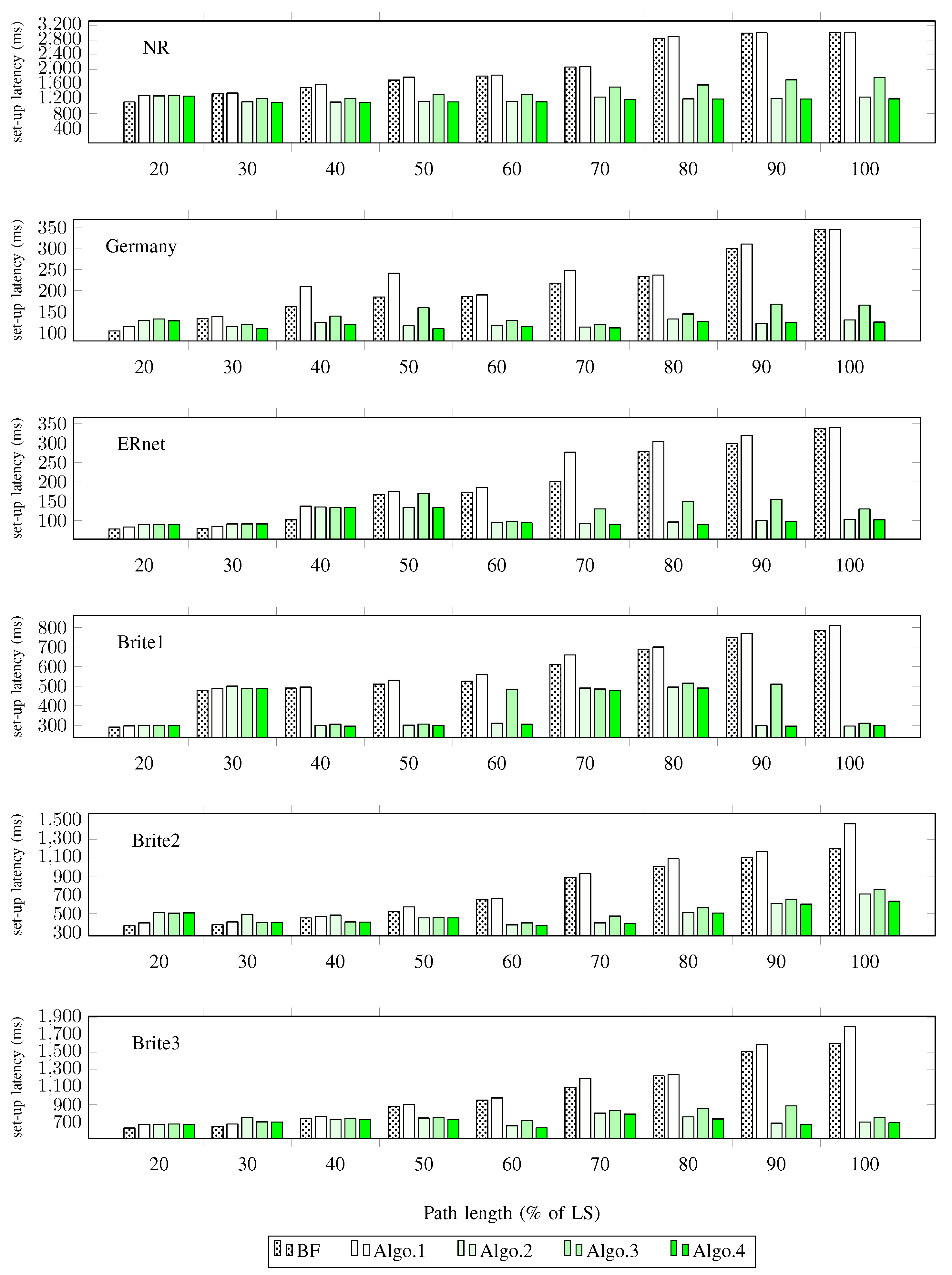
The experiment started by taking a network topology as an input. Then, 9 random paths with different sizes were captured. This was to ensure that the measurements were consistent with the design of the previous measurements. Two virtual hosts, namely H and H, were established for the purpose of sending and receiving network data packets. H was attached to the path source router and H was attached to the path destination router . In order to measure an IP packet’s end-to-end delay, the ARP cache is manually specified, hence, no ARP requests or responses are sent through the input network. An IP packet is first sent from the source, H, to the destination, H, and then the end-to-end delay is measured. Afterwards, a random link connecting any two neighbours belonging to the captured path is selected in order to simulate a link failure. Finally, a different IP packet from H to H is generated to measure end-to-end delay, following the random link failure. The experiment was carried out in two contexts. First, the path chosen had a normal condition, but the routers belonging to the path did not have rules to forward incoming packets. As a result, the controller would need to interact with all its routers to set-up appropriate flow entries. The second context had a path that was abnormal, in that it contained a link failure, as illustrated in Step 5 of Figure 9. The routers along the abnormal path already have flow entries for forwarding incoming packets. However, such packets are not able to follow the path due to the presence of the failure. In this scenario, the controller needs to be referenced in order to divert incoming packets away from the failed link. Such a diversion required the insertion and deletion of a number of flow entries. Figure 10 shows the set-up latency achieved by Algorithms 1–4 versus the percentage of path length for all the simulated topologies. The dotted bar, that is, BF, represents the installation time of the selected path before the failure occurs. Inclusion of this approach allowed us to identify the extent to which the proposed algorithms were capable of finding an alternative path in the shortest time.
We observed that the set-up time for an alternative path achieved by Algorithm 1 was either equal to or slightly higher than the time required to install the path before a failure, that is, BF. This was due to the fact that in Algorithm 1, alternative paths had either equal or longer length than primary paths. In addition, the path set-up latencies were affected by the network topology size. Paths in large topologies took longer to be establish than those in small topologies. This was because the flow entry set-up latencies were higher in large networks than in small ones [44].
On the other hand, the performance of the proposed algorithms improved when the length of the paths increased. In terms of the set-up time, Table 5 presents the relative difference in the performance of Algorithms 2–4 in comparison to Algorithm 1. The relative difference is the percentage of increase or decrease in set-up time between the proposed approaches and Algorithm 1. The downwards arrow next to the percentage values of Table 5 indicates the decrease in set-up time while the upwards arrow indicates the increase. When the percentage path length was 20–30% the proposed algorithms mostly produced a slight increase in the time required to install alternative paths. In fact, the increase was less than 10% in most cases and 27% in the worst case. In contrast, the proposed approaches reduced the required time to install the alternative paths when the path length ranged from 40% to 100%. The reduction ratio was up to 70% for long paths and up to 40% for medium length ones. The reduction rate of Algorithms 2 and 3 was relatively better than that of Algorithm 4. This was due to the fact that in Algorithm 4, only half of the path’s flow entries needed to be replaced. Finally, this latency measurement demonstrated the ability of the proposed approaches to reduce alternative paths’ set-up times, particularly, for long and medium length paths.
We have evaluated our path recovery algorithms under the headings: length, operation and latency. The proposed approaches do not come with the guarantee that the optimal shortest path will be found. However, experiments demonstrated that in general the increase in the path length cost was small compared to Dijkstra’s algorithm. A slight increase in the cost of path installation for short paths was observed, but for long and medium paths, the proposed approaches were more efficient, and achieved a good reduction in path installation cost. We posit that a promising next step is to consider how prediction algorithms that predict the occurrence of future link failures could be used to selectively, proactively perform path recovery ahead of time. In related work in Reference [45], we considered how to pose quality of delivery metric prediction as a machine learning problem. Similarly, in the context of data-centre networks which rapid path recovery is crucially important [46], we showed that better estimators of network state could be used to dynamically adjust flow tables according to network state as opposed to just link failures. What is clear is that prediction algorithms, based on these types of approaches for example, will provide a key component in future attempts to speed-up path restoration techniques. Lastly, the experimental network topologies of this work have a relatively high density, that is, average nodal degree , where this is common in Europe. We will study the behaviour of our proposed algorithms in networks where the average node degree is <3, such as those commonly deployed in North America and Asia.
6. Conclusions
In this paper, we investigated the problem of restoring paths in a manner which had low operation and installation costs. The motivation for this work was that conventional techniques based on shortest path restoration, did not guarantee the fastest recovery. To solve this problem we proposed two novel families of approaches, a Community Detection based approach and a Path Anatomy based approach, for the purpose of reducing the number of operations required for path restoration. From the perspective of a practitioner, reducing the path recovery time is important as this accelerates the process of recovering from a link failure. As way-points to achieving our rapid path recovery objective we contributed (1) a graph- and set-theory based formulation of the problem and solution; (2) a new system framework based was developed to represent the technical part of the proposed methods; and finally (3) an extensive performance analysis of the path recovery techniques was conducted. Our experiments were conducted on real and synthetic network topologies which gives credence to the following claims. Experiments demonstrated that in general the increase in the path length cost was small compared to Dijkstra’s algorithm. The proposed approaches slightly increased the cost of path installation for short paths (i.e., 3 nodes and less) in some cases. However, they were more efficient in achieving a good reduction in the path installation cost for long and medium length paths. Finally, the proposed approaches differ from the existing techniques by having the network reconfigured quickly rather than optimally for the sake of rapid restoration and this can be seen as an advantage when the network operates in a harsh environment.
Author Contributions
Conceptualization, A.M.; Methodology, A.M.; Software, A.M.; Validation, A.M. and R.d.F.; Investigation, R.d.F. and B.A.; Resources, A.M. and R.d.F.; Data curation, A.M., R.d.F. and B.A.; Writing original draft preparation, A.M.; Project administration, A.M., R.d.F. and B.A.; Visualization, Malik, R.d.F. and B.A.; Supervision, R.d.F. and B.A.; Writing review and editing, R.d.F. and B.A.; Funding acquisition, R.d.F. All authors have read and agreed to the published version of the manuscript.
Funding
This publication has emanated from research conducted with the financial support of Science Foundation Ireland (SFI) under the Grant Number 15/SIRG/3459.
Conflicts of Interest
The authors declare no conflict of interest.
References
- Koponen, T.; Shenker, S.; Balakrishnan, H.; Feamster, N.; Ganichev, I.; Ghodsi, A.; Godfrey, P.; McKeown, N.; Parulkar, G.; Raghavan, B.; et al. Architecting for innovation. ACM SIGCOMM Comput. Commun. Rev. 2011, 41, 24–36. [Google Scholar] [CrossRef]
- Zaidi, Z.; Friderikos, V.; Yousaf, Z.; Fletcher, S.; Dohler, M.; Aghvami, H. Will SDN be part of 5G? IEEE Commun. Surv. Tutor. 2018, 20, 3220–3258. [Google Scholar] [CrossRef] [Green Version]
- Akyildiz, I.F.; Lee, A.; Wang, P.; Luo, M.; Chou, W. A roadmap for traffic engineering in SDN-OpenFlow networks. Comput. Netw. 2014, 71, 1–30. [Google Scholar] [CrossRef]
- Vasseur, J.P.; Pickavet, M.; Demeester, P. Network Recovery: Protection and Restoration of Optical, SONET-SDH, IP, and MPLS; Elsevier: Amsterdam, The Netherlands, 2004. [Google Scholar]
- Komajwar, S.; Korkmaz, T. Challenges and solutions to consistent data plane update in software defined networks. Comput. Commun. 2018, 130, 50–59. [Google Scholar] [CrossRef]
- Markopoulou, A.; Iannaccone, G.; Bhattacharyya, S.; Chuah, C.N.; Ganjali, Y.; Diot, C. Characterization of failures in an operational IP backbone network. IEEE/ACM Trans. Netw. (TON) 2008, 16, 749–762. [Google Scholar] [CrossRef]
- De Fréin, R.; Pfaff, J.; Paré, T. Enterprise Data Center Globality Measurement. In Proceedings of the 2015 IEEE International Conference on Computer and Information Technology; Ubiquitous Computing and Communications; Dependable, Autonomic and Secure Computing; Pervasive Intelligence and Computing, Liverpool, UK, 26–28 October 2015; pp. 1861–1869. [Google Scholar] [CrossRef] [Green Version]
- Sharma, S.; Staessens, D.; Colle, D.; Pickavet, M.; Demeester, P. Enabling fast failure recovery in OpenFlow networks. In Proceedings of the 2011 8th International Workshop on the Design of Reliable Communication Networks (DRCN), Krakow, Poland, 10–12 October 2011; pp. 164–171. [Google Scholar]
- Staessens, D.; Sharma, S.; Colle, D.; Pickavet, M.; Demeester, P. Software defined networking: Meeting carrier grade requirements. In Proceedings of the 2011 18th IEEE Workshop on Local & Metropolitan Area Networks (LANMAN), Chapel Hill, NC, USA, 13–14 October 2011; pp. 1–6. [Google Scholar]
- Kúniar, M.; Perešíni, P.; Vasić, N.; Canini, M.; Kostić, D. Automatic failure recovery for software-defined networks. In Proceedings of the Second ACM SIGCOMM Workshop on Hot Topics in Software Defined Networking, Hong Kong, China, 16 August 2013; pp. 159–160. [Google Scholar]
- Philip, V.D.; Gourhant, Y. Cross-control: A scalable multi-topology fault restoration mechanism using logically centralized controllers. In Proceedings of the 2014 IEEE 15th International Conference on High Performance Switching and Routing (HPSR), Vancouver, BC, Canada, 1–4 July 2014; pp. 57–63. [Google Scholar]
- Kim, H.; Schlansker, M.; Santos, J.R.; Tourrilhes, J.; Turner, Y.; Feamster, N. Coronet: Fault tolerance for software defined networks. In Proceedings of the 2012 20th IEEE International Conference on Network Protocols (ICNP), Austin, TX, USA, 30 October–2 November 2012; pp. 1–2. [Google Scholar]
- Dijkstra, E.W. A note on two problems in connexion with graphs. Numerische Mathematik 1959, 1, 269–271. [Google Scholar] [CrossRef] [Green Version]
- Jinyao, Y.; Hailong, Z.; Qianjun, S.; Bo, L.; Xiao, G. HiQoS: An SDN-based multipath QoS solution. China Commun. 2015, 12, 123–133. [Google Scholar]
- Malik, A.; Aziz, B.; Adda, M.; Ke, C.H. Smart routing: Towards proactive fault handling of software-defined networks. Comput. Netw. 2020, 170, 107104. [Google Scholar] [CrossRef] [Green Version]
- Perner, C.; Carle, G. Comparison of Optimization Goals for Resilient Routing. In Proceedings of the 2019 IEEE International Conference on Communications Workshops (ICC Workshops), Shanghai, China, 20–24 May 2019; pp. 1–6. [Google Scholar]
- Perner, C. Network optimization for safety-critical systems using software-defined networks. In International Conference on Architecture of Computing Systems; Springer: Berlin/Heidelberg, Germany, 2018; pp. 127–138. [Google Scholar]
- Astaneh, S.A.; Heydari, S.S. Optimization of SDN flow operations in multi-failure restoration scenarios. IEEE Trans. Netw. Serv. Manag. 2016, 13, 421–432. [Google Scholar] [CrossRef]
- Cheng, Z.; Zhang, X.; Li, Y.; Yu, S.; Lin, R.; He, L. Congestion-aware local reroute for fast failure recovery in software-defined networks. IEEE/OSA J. Opt. Commun. Netw. 2017, 9, 934–944. [Google Scholar] [CrossRef]
- Gotani, K.; Takahira, H.; Hata, M.; Guillen, L.; Izumi, S.; Abe, T. OpenFlow Based Information Flow Control Considering Route Switching Cost. In Proceedings of the 2019 IEEE 43rd Annual Computer Software and Applications Conference (COMPSAC), Milwaukee, WI, USA, 15–19 July 2019; Volume 2, pp. 527–530. [Google Scholar]
- Gotani, K.; Takahira, H.; Hata, M.; Guillen, L.; Izumi, S.; Abe, T.; Suganuma, T. Design of an SDN Control Method Considering the Path Switching Time under Disaster Situations. In Proceedings of the 2018 5th International Conference on Information and Communication Technologies for Disaster Management (ICT-DM), Sendai, Japan, 4–7 December 2018; pp. 1–4. [Google Scholar]
- Akyildiz, I.F.; Su, W.; Sankarasubramaniam, Y.; Cayirci, E. Wireless sensor networks: A survey. Comput. Netw. 2002, 38, 393–422. [Google Scholar] [CrossRef] [Green Version]
- Moshref, M.; Yu, M.; Sharma, A.; Govindan, R. vcrib: Virtualized rule management in the cloud. In Proceedings of the HotCloud ’12, Boston, MA, USA, 12–13 June 2012. [Google Scholar]
- Ramarao, K. A simple variant of node connectivity is NP-complete. Int. J. Comput. Math. 1986, 20, 245–251. [Google Scholar] [CrossRef]
- Fortunato, S. Community detection in graphs. Phys. Rep. 2010, 486, 75–174. [Google Scholar] [CrossRef] [Green Version]
- Yang, B.; Liu, D.; Liu, J. Discovering communities from social networks: Methodologies and applications. In Handbook of Social Network Technologies and Applications; Springer: Berlin/Heidelberg, Germany, 2010; pp. 331–346. [Google Scholar]
- Plantié, M.; Crampes, M. Survey on social community detection. In Social Media Retrieval; Springer: Berlin/Heidelberg, Germany, 2013; pp. 65–85. [Google Scholar]
- Rosset, V.; Paulo, M.A.; Cespedes, J.G.; Nascimento, M.C. Enhancing the reliability on data delivery and energy efficiency by combining swarm intelligence and community detection in large-scale WSNs. Expert Syst. Appl. 2017, 78, 89–102. [Google Scholar] [CrossRef]
- Hui, P.; Sastry, N. Real world routing using virtual world information. In Proceedings of the 2009 International Conference on Computational Science and Engineering, Vancouver, BC, Canada, 29–31 August 2009; Volume 4, pp. 1103–1108. [Google Scholar]
- De Maesschalck, S.; Colle, D.; Lievens, I.; Pickavet, M.; Demeester, P.; Mauz, C.; Jaeger, M.; Inkret, R.; Mikac, B.; Derkacz, J. Pan-European optical transport networks: An availability-based comparison. Photonic Netw. Commun. 2003, 5, 203–225. [Google Scholar] [CrossRef]
- Girvan, M.; Newman, M.E. Community structure in social and biological networks. Proc. Natl. Acad. Sci. USA 2002, 99, 7821–7826. [Google Scholar] [CrossRef] [Green Version]
- Shalimov, A.; Zuikov, D.; Zimarina, D.; Pashkov, V.; Smeliansky, R. Advanced study of SDN/OpenFlow controllers. In Proceedings of the 9th Central & Eastern European Software Engineering Conference, Moscow, Russia, 23–25 October 2013; p. 1. [Google Scholar]
- McKeown, N.; Anderson, T.; Balakrishnan, H.; Parulkar, G.; Peterson, L.; Rexford, J.; Shenker, S.; Turner, J. OpenFlow: Enabling innovation in campus networks. ACM SIGCOMM Comput. Commun. Rev. 2008, 38, 69–74. [Google Scholar] [CrossRef]
- POX Wiki. Openflow.Discovery. 2014. Available online: https://openflow.stanford.edu/display/ONL/POX+Wiki.html#POXWiki-forwarding.l2_learning (accessed on 1 May 2020).
- Hagberg, A.; Swart, P.; S Chult, D. Exploring Network Structure, Dynamics, and Function Using NetworkX; Technical Report; Los Alamos National Lab.: Los Alamos, NM, USA, 2008. [Google Scholar]
- Csardi, G.; Nepusz, T. The igraph software package for complex network research. InterJournal Complex Syst. 2006, 1695, 1–9. [Google Scholar]
- Orlowski, S.; Wessäly, R.; Pióro, M.; Tomaszewski, A. SNDlib 1.0—Survivable network design library. Networks 2010, 55, 276–286. [Google Scholar] [CrossRef] [Green Version]
- Rossi, R.A.; Ahmed, N.K. The Network Data Repository with Interactive Graph Analytics and Visualization. In Proceedings of the Twenty-Ninth AAAI Conference on Artificial Intelligence, Austin, Texas, 25–29 January 2015; pp. 4292–4293. [Google Scholar]
- Medina, A.; Lakhina, A.; Matta, I.; Byers, J. BRITE: Universal Topology Generation from a User’s Perspective; Technical Report; Boston University Computer Science Department: Boston, MA, USA, 2001. [Google Scholar]
- Waxman, B.M. Routing of multipoint connections. IEEE J. Sel. Areas Commun. 1988, 6, 1617–1622. [Google Scholar] [CrossRef]
- Lantz, B.; Heller, B.; McKeown, N. A network in a laptop: Rapid prototyping for software-defined networks. In Proceedings of the 9th ACM SIGCOMM Workshop on Hot Topics in Networks, New York, NY, USA, 20–21 October 2010; pp. 1–6. [Google Scholar]
- Kreutz, D.; Ramos, F.M.; Verissimo, P.E.; Rothenberg, C.E.; Azodolmolky, S.; Uhlig, S. Software-defined networking: A comprehensive survey. Proc. IEEE 2014, 103, 14–76. [Google Scholar] [CrossRef] [Green Version]
- Clauset, A.; Newman, M.E.; Moore, C. Finding community structure in very large networks. Phys. Rev. E 2004, 70, 066111. [Google Scholar] [CrossRef] [PubMed] [Green Version]
- Khalili, R.; Despotovic, Z.; Hecker, A. Flow Setup Latency in SDN Networks. IEEE J. Sel. Areas Commun. 2018, 36, 2631–2639. [Google Scholar] [CrossRef]
- De Fréin, R. Source Separation Approach to Video Quality Prediction in Computer Networks. IEEE Commun. Lett. 2016, 20, 1333–1336. [Google Scholar] [CrossRef]
- De Fréin, R. The data-centre whisperer: Relative attribute usage estimation for cloud servers. In Proceedings of the 2016 24th European Signal Processing Conference (EUSIPCO), Budapest, Hungary, 29 August–2 September 2016; pp. 687–691. [Google Scholar] [CrossRef]
Figure 1.
Illustration of community detection and graph partitioning process: A good solution (RHS) has a high number of links between members of the same community and a low number of links to other communities.
Figure 1.
Illustration of community detection and graph partitioning process: A good solution (RHS) has a high number of links between members of the same community and a low number of links to other communities.

Figure 2.
Running community detection on the European Reference network topology (ERnet) yields five communities. Colours followed by pairs of integers denote the names of the communities and the number of inter and intra community links. For example the red community has 4 inter community links and 7 intra-community links, Red (4,7). The remaining communities are summarized: Blue (5,9), Green (4,8), Orange (8,10) and Yellow (4,6).

Figure 3.
In a path anatomy the sequence of routers that form the path can be partitioned into two sub-paths which have equal length. Recovery can be achieved by either reconfiguring the flow tables associated with the half of the path which contains the failure, or the link which has failed.
Figure 3.
In a path anatomy the sequence of routers that form the path can be partitioned into two sub-paths which have equal length. Recovery can be achieved by either reconfiguring the flow tables associated with the half of the path which contains the failure, or the link which has failed.

Figure 4.
Proposed framework components: the primary contribution of this paper lies in the Community Detection and the Path Anatomy blocks. Openflow is used on the southbound interface and POX python APIs are used on the northbound interface. The framework components are labelled with the algorithms that describe their function.
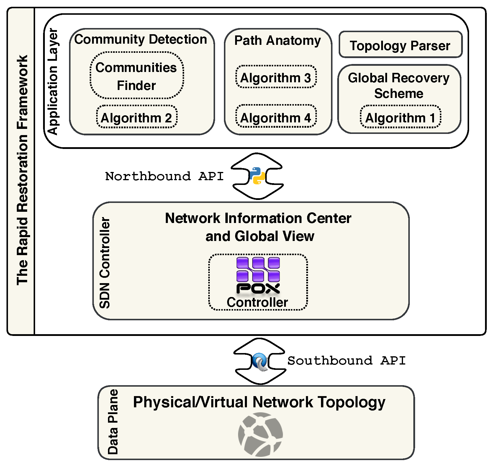
Figure 5.
The topologies used to evaluate rapid recovery techniques are illustrated. We evaluate recovery algorithms in terms of their length, operation and latency. The densities of theses topologies are listed in Table 1.
Figure 5.
The topologies used to evaluate rapid recovery techniques are illustrated. We evaluate recovery algorithms in terms of their length, operation and latency. The densities of theses topologies are listed in Table 1.
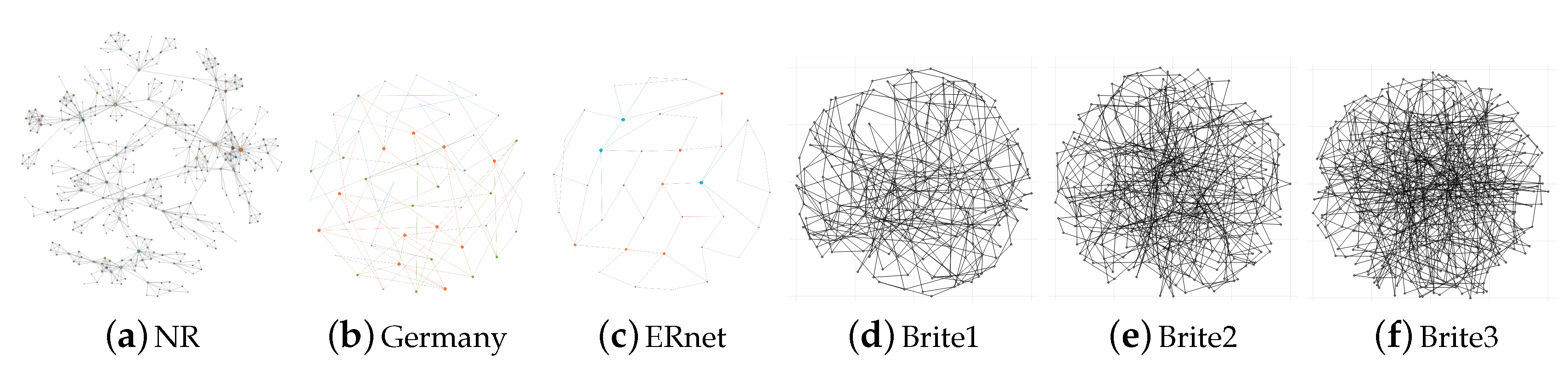
Figure 6.
The average path cost, that is, number of hops, achieved by Algorithms 1–4 for the experimental topologies of Table 1.
Figure 6.
The average path cost, that is, number of hops, achieved by Algorithms 1–4 for the experimental topologies of Table 1.

Figure 7.
Flowchart for calculating Success and Fail variables.

Figure 8.
The average path operation cost, that is, number of add & remove entries, achieved by Algorithms 1–4 for the experimental topologies of Table 1.
Figure 8.
The average path operation cost, that is, number of add & remove entries, achieved by Algorithms 1–4 for the experimental topologies of Table 1.

Figure 9.
Process of measuring the cost of path installation.

Figure 10.
The path set-up latency, that is, time required to install the network path, achieved by Algorithms 1–4 for the experimental topologies of Table 1 are illustrated as a function of the normalized path length.
Figure 10.
The path set-up latency, that is, time required to install the network path, achieved by Algorithms 1–4 for the experimental topologies of Table 1 are illustrated as a function of the normalized path length.

Table 1.
Topology characteristics: The topologies examined had different node and edge counts, and diameters and densities.
Table 1.
Topology characteristics: The topologies examined had different node and edge counts, and diameters and densities.
| Topology | Nodes | Edges | Diameter | Density |
|---|---|---|---|---|
| NR | 379 | 914 | 17 | 0.0127598 |
| Germany | 50 | 88 | 9 | 0.0718367 |
| ERnet | 37 | 57 | 8 | 0.0855855 |
| Brite1 | 200 | 400 | 8 | 0.0201005 |
| Brite2 | 300 | 600 | 8 | 0.0133779 |
| Brite3 | 400 | 800 | 7 | 0.0100250 |
Table 2.
Average path costs (averaged across all topologies) achieved by Algorithms 1–4 are rounded.
Table 2.
Average path costs (averaged across all topologies) achieved by Algorithms 1–4 are rounded.
| % | 20 | 30 | 40 | 50 | 60 | 70 | 80 | 90 | 100 |
|---|---|---|---|---|---|---|---|---|---|
| NR | 4 | 6 | 8 | 11 | 12 | 13 | 15 | 16 | 19 |
| Germany | 3 | 4 | 5 | 6 | 6 | 7 | 8 | 9 | 10 |
| ERnet | 4 | 4 | 5 | 6 | 7 | 8 | 8 | 9 | 10 |
| Brite1 | 3 | 3 | 4 | 5 | 6 | 8 | 8 | 9 | 9 |
| Brite2 | 3 | 3 | 4 | 6 | 7 | 8 | 8 | 9 | 11 |
| Brite3 | 3 | 3 | 5 | 5 | 6 | 8 | 8 | 9 | 10 |
| Average | 3 | 4 | 5 | 7 | 7 | 9 | 9 | 10 | 12 |
Table 3.
Completion rate, link density and modularity achieved by Algorithm 3 for all topologies.
| Completion Rates | |||||||
|---|---|---|---|---|---|---|---|
| Network | Communities | Intra Links | Inter Links | Intra Links Density | Success Rate | Fail Rate | Modularity |
| NR | 18 | 852 | 62 | 93.21% | 97% | 3% | 0.838 |
| Germany | 6 | 68 | 20 | 77.27% | 96% | 4% | 0.597 |
| ERnet | 5 | 44 | 13 | 77.19% | 93% | 7% | 0.533 |
| Brite1 | 9 | 263 | 137 | 65.75% | 80.7% | 19.3% | 0.530 |
| Brite2 | 13 | 360 | 240 | 60% | 69.4% | 30.6% | 0.506 |
| Brite3 | 11 | 496 | 304 | 62% | 75.3% | 24.7% | 0.515 |
Table 4.
Average cost reduction rate of Algorithms 1–3 are compared as a function of the normalized path length.
Table 4.
Average cost reduction rate of Algorithms 1–3 are compared as a function of the normalized path length.
| Path Length | ||||||||||
|---|---|---|---|---|---|---|---|---|---|---|
| 20% | 30% | 40% | 50% | 60% | 70% | 80% | 90% | 100% | ||
| Algorithm 2 | NR | 44.4 | 61.5 | 70.5 | 76.1 | 78.2 | 80.7 | 83.8 | 84.8 | 86.8 |
| Germany | 28.5 | 44.4 | 50 | 58.3 | 58.3 | 64.2 | 68.7 | 72.2 | 75 | |
| ERnet | 14.2 | 14.2 | 33.3 | 40 | 50 | 57.1 | 57.1 | 62.5 | 66.6 | |
| Brite1 | 16.6 | 16.6 | 37.5 | 50 | 58.3 | 57.1 | 57.1 | 62.5 | 72.2 | |
| Brite2 | - | - | - | 30 | 33.3 | 42.8 | 48.8 | 50 | 55.5 | |
| Brite3 | 28.5 | 28.5 | 37.5 | 50 | 58.3 | 64.2 | 57.1 | 62.5 | 61.1 | |
| Algorithm 3 | NR | 33.3 | 38.4 | 41.1 | 42.8 | 43.4 | 46.1 | 48.3 | 48.4 | 47.3 |
| Germany | 28.5 | 33.3 | 30 | 41.6 | 41.6 | 35.7 | 43.7 | 44.4 | 45 | |
| ERnet | 14.2 | 14.2 | 22.2 | 30 | 33.3 | 35.7 | 35.7 | 37.5 | 38.8 | |
| Brite1 | 16.6 | 16.6 | 25 | 30 | 41.6 | 35.7 | 35.7 | 43.7 | 38.8 | |
| Brite2 | 14.2 | - | 25 | 30 | 41.6 | 35.7 | 35.7 | 43.7 | 38.3 | |
| Brite3 | 14.2 | 14.2 | 25 | 30 | 41.6 | 35.7 | 35.7 | 43.7 | 44.4 | |
| Algorithm 4 | NR | 44.4 | 61.5 | 70.5 | 76.1 | 78.2 | 80.7 | 83.8 | 84.8 | 86.8 |
| Germany | 28.5 | 44.4 | 50 | 58.3 | 58.3 | 64.2 | 68.7 | 72.2 | 75 | |
| ERnet | 14.2 | 14.2 | 33.3 | 40 | 50 | 57.1 | 57.1 | 62.5 | 66.6 | |
| Brite1 | 16.6 | 16.6 | 37.5 | 40 | 58.3 | 57.1 | 57.1 | 68.7 | 72.2 | |
| Brite2 | 14.2 | - | 25 | 40 | 50 | 50 | 50 | 56.2 | 61.1 | |
| Brite3 | 28.5 | 28.5 | 25 | 50 | 50 | 50 | 50 | 56.2 | 61.1 | |
Table 5.
Set-up reduction rate of Algorithms 2–4 for each topology as a function of the normalized path length.
Table 5.
Set-up reduction rate of Algorithms 2–4 for each topology as a function of the normalized path length.
| Path Length | ||||||||||
|---|---|---|---|---|---|---|---|---|---|---|
| 20% | 30% | 40% | 50% | 60% | 70% | 80% | 90% | 100% | ||
| Algorithm 2 | NR | 0.9 ↓ | 10.2 ↓ | 30.5 ↓ | 36.9 ↓ | 38.9 ↓ | 39.7 ↓ | 58.6 ↓ | 59.6 ↓ | 58.6 ↓ |
| Germany | 13 ↑ | 17.2 ↓ | 40.4 ↓ | 51.4 ↓ | 37.8 ↓ | 54 ↓ | 43.8 ↓ | 60.3 ↓ | 62 ↓ | |
| ERnet | 8.4 ↑ | 8.3 ↑ | 1.4 ↓ | 23.4 ↓ | 48.6 ↓ | 66.3 ↓ | 68.4 ↓ | 68.7 ↓ | 69.7 ↓ | |
| Brite1 | 0.3 ↑ | 2.4 ↑ | 39.8 ↓ | 43.4 ↓ | 44.6 ↓ | 27.7 ↓ | 29.2 ↓ | 61.3 ↓ | 63.4 ↓ | |
| Brite2 | 27 ↑ | 19.5 ↑ | 2.7 ↑ | 21 ↓ | 27.4 ↓ | 56.9 ↓ | 53.2 ↓ | 48.2 ↓ | 51.7 ↓ | |
| Brite3 | 0.3 ↑ | 11.1 ↑ | 4.2 ↓ | 17.2 ↓ | 32.8 ↓ | 33.3 ↓ | 39.1 ↓ | 60 ↓ | 61.1 ↓ | |
| Algorithm 3 | NR | 0.5 ↑ | 11.4 ↓ | 24.3 ↓ | 26.2 ↓ | 29.1 ↓ | 26.7 ↓ | 45.5 ↓ | 42.6 ↓ | 41 ↓ |
| Germany | 15.6 ↑ | 13.6 ↓ | 33.3 ↓ | 33.6 ↓ | 31.5 ↓ | 51.6 ↓ | 38.8 ↓ | 45.8 ↓ | 51.8 ↓ | |
| ERnet | 8.4 ↑ | 8.3 ↑ | 2.9 ↓ | 2.8 ↓ | 47 ↓ | 52.9 ↓ | 50.6 ↓ | 51.5 ↓ | 61.7 ↓ | |
| Brite1 | 0.6 ↑ | 0.2 ↑ | 38.3 ↓ | 42.2 ↓ | 13.7 ↓ | 26.5 ↓ | 26.4 ↓ | 33.8 ↓ | 61.7 ↓ | |
| Brite2 | 27.5 ↑ | 1.7 ↑ | 12.2 ↓ | 20.1 ↓ | 39.3 ↓ | 49.4 ↓ | 48.6 ↓ | 44.4 ↓ | 48.3 ↓ | |
| Brite3 | 0.7 ↑ | 3.7 ↑ | 3.5 ↓ | 16.5 ↓ | 26.8 ↓ | 30.8 ↓ | 31.7 ↓ | 44.3 ↓ | 58.3 ↓ | |
| Algorithm 4 | NR | 1.3 ↓ | 19.1 ↓ | 30.6 ↓ | 37.4 ↓ | 39.4 ↓ | 42.6 ↓ | 58.7 ↓ | 60.1 ↓ | 60.2 ↓ |
| Germany | 12.1 ↑ | 20.8 ↓ | 42.8 ↓ | 54.3 ↓ | 39.4 ↓ | 54.8 ↓ | 46.4 ↓ | 59.6 ↓ | 63.4 ↓ | |
| ERnet | 8.4 ↑ | 8.3 ↑ | 2.1 ↓ | 24 ↓ | 49.1 ↓ | 48.8 ↓ | 70.3 ↓ | 69.3 ↓ | 70 ↓ | |
| Brite1 | 0.3 ↑ | 0.2 ↑ | 40.4 ↓ | 43.5 ↓ | 45.5 ↓ | 27.2 ↓ | 30 ↓ | 61.7 ↓ | 63 ↓ | |
| Brite2 | 26.2 ↑ | 1.9 ↓ | 12.6 ↓ | 20.8 ↓ | 43.9 ↓ | 58 ↓ | 53.8 ↓ | 48.8 ↓ | 57.1 ↓ | |
| Brite3 | 0.1 ↑ | 3.5 ↑ | 4.8 ↓ | 18.8 ↓ | 35.3 ↓ | 34.1 ↓ | 41 ↓ | 57.8 ↓ | 61.6 ↓ | |
© 2020 by the authors. Licensee MDPI, Basel, Switzerland. This article is an open access article distributed under the terms and conditions of the Creative Commons Attribution (CC BY) license (http://creativecommons.org/licenses/by/4.0/).
Share and Cite
MDPI and ACS Style
Malik, A.; de Fréin, R.; Aziz, B. Rapid Restoration Techniques for Software-Defined Networks. Appl. Sci. 2020, 10, 3411. https://doi.org/10.3390/app10103411
AMA Style
Malik A, de Fréin R, Aziz B. Rapid Restoration Techniques for Software-Defined Networks. Applied Sciences. 2020; 10(10):3411. https://doi.org/10.3390/app10103411
Chicago/Turabian StyleMalik, Ali, Ruairí de Fréin, and Benjamin Aziz. 2020. "Rapid Restoration Techniques for Software-Defined Networks" Applied Sciences 10, no. 10: 3411. https://doi.org/10.3390/app10103411
Note that from the first issue of 2016, this journal uses article numbers instead of page numbers. See further details here.