Automatic Classification of Morphologically Similar Fish Species Using Their Head Contours


1
Data and Signal Processing Group, University of Vic—Central University of Catalonia, 08500 Vic, Catalonia, Spain
2
Institut de Ciències del Mar, ICM (CSIC), 08003 Barcelona, Catalonia, Spain
*
Authors to whom correspondence should be addressed.
Appl. Sci. 2020, 10(10), 3408; https://doi.org/10.3390/app10103408
Submission received: 26 March 2020
/
Revised: 10 May 2020
/
Accepted: 12 May 2020
/
Published: 14 May 2020
(This article belongs to the Special Issue Machine Learning Methods with Noisy, Incomplete or Small Datasets)
Abstract
:This work deals with the task of distinguishing between different Mediterranean demersal species of fish that share a remarkably similar form and that are also used for the evaluation of marine resources. The experts who are currently able to classify these types of species do so by considering only a segment of the contour of the fish, specifically its head, instead of using the entire silhouette of the animal. Based on this knowledge, a set of features to classify contour segments is presented to address both a binary and a multi-class classification problem. In addition to the difficulty present in successfully discriminating between very similar forms, we have the limitation of having small, unreliably labeled image data sets. The results obtained were comparable to those obtained by trained experts.
1. Introduction
Being able to determine the differences in shape between closely related fish species not only has an impact on fisheries and their management but also is essential for a variety of studies on marine ecology, genetics, phylogeny, biological invasion, and anthropogenic impact on the environment, among others [1]. All of these studies require the correct identification of a wide range of species, and the automatic classification of such species from images is still an open problem. The correct identification of many specimens of these sympatric species requires an experienced observer and is a highly time-consuming task; otherwise, many misclassification errors occur.
This paper focuses on two cases in which this problem appears. The first case deals with the separation between Red Mullets, (Mullus barbatus and Mullus surmuletus), and it will be treated as a binary classification problem. The second case is a multiclassification problem in which different species of Gurnard Chelidonichthys cuculus, Chelidonichthys lucerna, Chelidonichthys obscurus, Eutrigla gurnardus, Lepidotrigla cavillone, Lepidotrigla dieuzeidei, Peristedion cataphractum, Trigla lyra, and Trigloporus lastoviza are involved. Red Mullets and Gurnards are commonly caught and sold in fish markets as a mixture of species (Figure 1).
The observation is that experts who can correctly classify individuals of these species of fish by using shape characteristics—instead of considering the entire silhouette, represented as a closed contour- identify them by focusing on a specific contour fragment. They disregard the remaining part of the contour as they realise that it is irrelevant for classification purposes. This is because the discarded contour part provides information on variations within individuals of the same species with respect to age, size, sex or body condition, but does not provide information on the intrinsic characteristics involved in the distinction between species. The challenge for automated identification is to take these species-specific open contour fragments pointed out by the specialists to develop features that correctly identify the species automatically. In both cases considered in this work, experts mark the segment of interest of the profile as being the part that goes from the nose to the beginning of the dorsal fin of the fish.
The first case addressed deals with the binary classification of the Mullus network. Red Mullets (M. barbatus and M. surmuletus) are a major target as demersal fish species for the Mediterranean fish industry [2,3]. There are many comparative studies of these two species focusing on a range of topics, such as pollution bio-indicators, and fisheries or studies on age composition, growth, life history, feeding, genetics, ecology, and distribution [4,5,6,7,8,9]. As mentioned above, the evaluation of living resources requires the correct identification of species.
Searches for morphological features to help with the task of identifying these sympatric species have focused on characteristics, such as head and body measurements [10,11], barbells [12], dentition [13] or otoliths [14]. Amongst all of these biometric features, the angle of the head has been found to be one of the best diagnostic characteristics to distinguish between the two species, as the angle that the M. barbatus’head contour forms is more marked than that of M. surmuletus [10,15]. Even in fishery studies, however, the individual variability within Red Mullets causes identification problems and the only reliable distinction is the color pattern of their bent dorsal fin. However, it is not easy to obtain images of this feature from boat moorings in fishing harbours as the fish’s dorsal fin is folded. Furthermore, in most cases, the information on the fish caught that is given upon the arrival of the boat does not discriminate between both species of Red Mullets.
Thus, it is not possible to determine the statistics of individualized species of fish caught from the fishing industry, which adds error in the mathematical models of each species. In consequence, the correct identification of many specimens of these sympatric species requires an experienced observer and, as mentioned before, is a highly time-consuming task. A more complex case occurs in Mediterranean Gurnard fish (in the family of triglids and peristids), consisting of nine sympatric species (C. cuculus, C. lucerna, C. obscurus, E. gurnardus, L. cavillone, L. dieuzeidei, P. cataphractum, T. lyra, and T. lastoviza), which are fished through trawl fishing on continental shelves and upper slopes, and are usually considered as only one species or an unidentified mix of species in commercial capture statistics (Fisheries Database of the Catalan Government). Morphological differences between species are based on trends of the lateral line, scale distribution, head shape and preorbital bones [15], and a high degree of expertise is required to classify triglid species.
To solve both classification problems, we used a traditional machine learning (ML) workflow to create the models, which are the trained programs that predict the outputs based on a set of given inputs, also called features. That implies the design of such features as a first step, followed by the task of training the model. Conventional ML techniques include support vector machines (SVM), ensembled methods, decision trees, and also the extreme learning machines (ELM) used in this work, among others. In this context, ELM performs very similarly to SVM, with the added advantage of having a much quicker training process in comparison. In contrast to ML, an approach based on deep learning (DL) techniques exists in which the algorithms automatically learn which of the features are useful. The term deep refers to the multiple layers the networks have between inputs and outputs. In order to train models with DL techniques, a large amount of tagged data is required, which is complicated in our case as we work with a small dataset.
Several parameterization strategies have been previously explored for closed contours, and therefore an abundance of literature is available. An important part of the transformed methods dealing with closed contours is based on the Fourier transform. Among those methods, elliptic Fourier descriptors (EDF) is one of the most popular ones. This method was introduced by Reference [16], and some variations have been introduced since. As applications that require shape quantification are present in a wide range of different fields, an extensive amount of these can be found [17,18,19,20].
Fourier methods applied to periodic sequences (which can be associated with closed contours) exhibit good information-packing properties in the sense that they concentrate most of the signal energy in a few coefficients. Those few coefficients are employed as features for classifying purposes. The problem under discussion cannot be solved if the specimens are treated by considering their entire silhouette independently of the contour description technique employed, as is the case of multiple spatial scales methods curvature scale space (CSS) [21,22,23], or from the discrete wavelet transform (DWT) [24].
Therefore, knowing how the specialists solve the problem, the approach that will be used will imitate the one used by these experts and thus only consider the contour fragments of interest. Unfortunately, in the context of shape analysis, there is less work done on open contours and discrete transforms. Something that is well known, however, is that Fourier-based methods do not work well when the sequences are not periodic [25].
Different approaches can be used to deal with segment contours (open contours). In Reference [26], a wavelet analysis with cubic B-spline bases was used in order to reduce disturbances and confine them around the discontinuities, and in Reference [27], the windowed short time Fourier transform (STFT) was employed. The main problem with most transformed methods, especially those using Fourier, is the characterisation of the ends of the segments, which, in the case of open contours, are seen as discontinuities. In Reference [28], a large number of open contour segment descriptors were compiled and compared with each other, but none were found to be related to discrete transforms. Certain discrete cosine transform (DCT) formulations work better when it comes to the ends of the segments, and therefore seem to be the most appropriate discrete transformation to use when dealing with open contours.
As far as we know, the DCT used in the morphometric analysis was first employed in Reference [29] for the analysis of ammonite ribs (shell features of an extinct order of cephalopods). In Reference [30], the DCT was also used for symmetric closed contours that were simultaneously represented with closed and open contours (by taking half of the closed contour) and analyzed by EFD and DCT, respectively. Recently, in Reference [31], DCT was employed to quantify open contours of organic shapes and thus evaluate the morphological disparity of male genital evolution in sibling species of Drosophila. The point (which will be developed later) is that some formulations of the discrete cosine transform (DCT) can deal with segment extremes better and can also simultaneously compact the energy of the signal in very few coefficients.
In this paper, an ML method is proposed to automatically classify very similar species with an accuracy comparable to that achieved by experts when they use images to identify the correct species. The method is used both in a binary and in a multi-class classification problem. The images contain two landmarks, one in the snout and one at the beginning of the dorsal fin, to limit the segment used by the experts. An added issue to the classification, which is very difficult if we do not have the information that the specialist uses to discriminate, is that we have very few correctly tagged images. We find this problem even more pronounced in the multi-class classification problem.
The addressed task is established under the framework of supervised classification with databases, as mentioned, of reduced dimensions, which implies that there are few available cases to train the classifiers. The proposed method takes advantage of the knowledge of specialists in the field. As the main contributions, we highlight the development of features to represent open contours in a compact way, and by taking advantage of the appropriate contour normalization, we show that it is possible to eliminate the Gibbs effect that appears with the discrete Fourier transform (DFT). The proposed segment standardization makes it possible—both for the DCT and the FFT—to describe open contours with a single sequence instead of two (one for each coordinate) while, in addition, allowing us to compare the segments independently of rotations and scale variations. It is also robust to the small imprecisions or the noise that can be introduced when finding the contour.
The work continues as follows. In Section 2, Materials and Methods, the following points are presented: the databases and the discrete transforms as well as the corresponding implicit sequence extension and its relation in the representation of open contours, the contour extraction procedure and normalization and the development of the features used. Additionally in that section, the training, classification, and cross-validation methods are explained. Section 3 is devoted to the Results. In Section 3.2, we show how with a convolutional neural network (CNN) trained to detect the region of interest determined by the points of the expert, the region of interest can also be determined automatically, thus demonstrating that the points are not required. Finally, Section 4 is devoted to our Conclusions.
2. Materials and Methods
2.1. Discrete Transforms and Signal Reconstructions from a Reduced Set of Coefficients
In the following two subsections, we show the direct and reverse expressions of the DCT and DFT transforms, and their particularities when reconstructing in an approximated way the original sequence using a limited number L of coefficients. The small set of those coefficients, used properly, will be employed to develop the features for the classifier. Intuitively, the set of L coefficients will be a good set of contour descriptors as long as and the samples of are very close to the original .
2.1.1. Discrete Cosine Transform (Type-II)
The DCT-II forward and backward expressions that relate the points with the transformed coefficients take the form:
where if and if . The approximate reconstruction of with the first L coefficients , L< N is:
where are N reconstructed samples.
2.1.2. Discrete Fourier Transform
The discrete Fourier transform (DFT) forward and backward expressions that relate the points with the transformed coefficients take the form:
In the DFT case, . Considering the well-known DFT property (symbol stands for complex conjugated) which holds for , the module and phase notation of as , and the Euler formula, the approximation of , , obtained from the first L coefficients , can be written as:
showing that .
2.1.3. A Note on the Implicit Extension of the Sequences Depending on the Discrete Transform Used and the Case of Open Contours
For a discrete transform, the way in which the sequence remains implicitly defined outside the main range is known as implicit extension. Any discrete transform has a particular way of extending the sequence. This can be seen from the backward transform expressions in (2) and in (5), for the DCT-II and the DFT, respectively. As the bases in these expressions are defined beyond , it follows that also remains implicitly defined beyond this range. When the approximation of by is done with few bases () as in Equations (3) and (6), the samples of near the main sequence extremes ( and ) tend to manifest the implicit periodicity of the transform. Depending on how a particular transformation extends the sequences at both extremes, more or less transformed coefficients will be required to have a quality approximation.
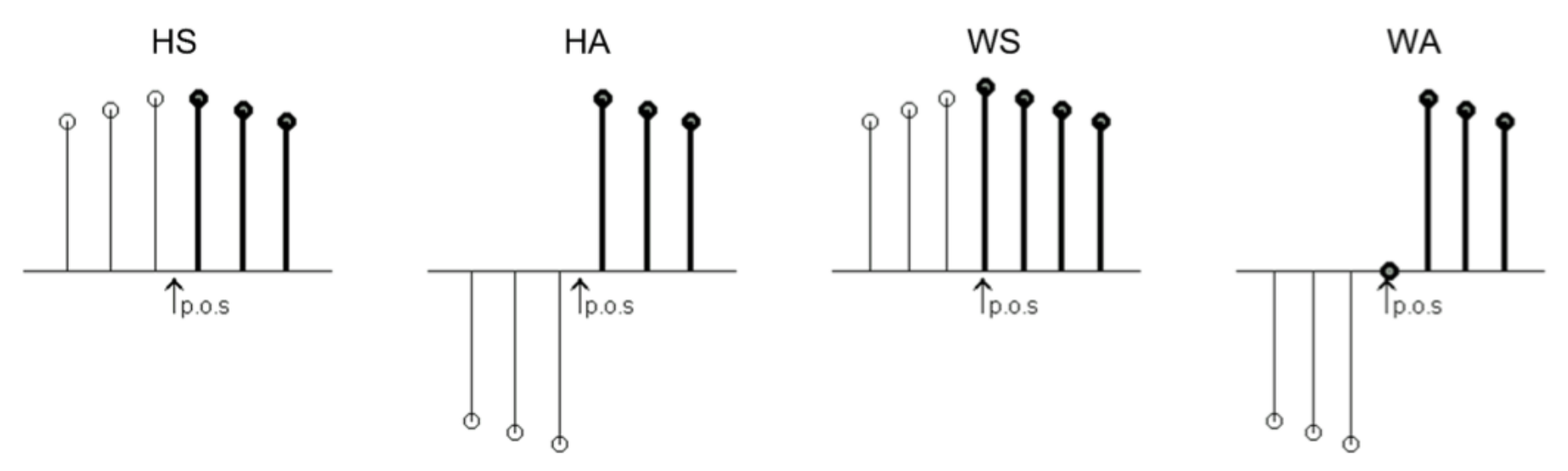
Let us first consider the DCT-II, which belongs to the family of discrete trigonometric transforms (DTT), and their implicit extension properties [32,33,34,35,36,37,38,39,40]. To summarize the DTT sequence extensions, two relevant parameters must be considered—the symmetry type (ST) and the point of symmetry (PoS). When it comes to the ST, the replication can be performed symmetrically (S) or anti-symmetrically (A). Considering that the samples of the sequence are equispaced, the PoS can be positioned either in the middle of the space between the elements, named half (H) sample or midpoint, or just at the position of the element, named whole (W) sample or meshpoint.
Thus, when considering a single point from an edge of a sequence, there are four options to extend the sequence, commonly denoted by two letters—(HS), (HA), (WS), and (WA). Figure 2 represents those four possibilities for the left edge of a main sequence, which is depicted in bold. Then, it follows that since all finite sequence have two edges, there are eight total possible combinations, each one of which is associated with one different formulation corresponding to either the DCT or the DST (discrete sine transform) groups [34,37,41,42].
The DTTs that best approximate open contours with few coefficients are those that have HS or WS implicit extensions on both extremes. That happens for the DCT formulation types -I, -II, -V, and -VI. In those cases, the sequence considered with implicit extensions does not lose continuity. In the particular case of the DCT-II, the continuity in both extremes is defined as and .
In the case of the DFT, it is easy to verify that . From (5) we have:
Thus, for the DFT, reconstructions with few coefficients are very efficient only when and are closed, as occurs in the case of objects with smooth contours. When , as and , the continuity is perceived in the extended sequence. However, DFT loses the property of compacting energy in few coefficients when a discontinuity appears as differs from , which usually is the case of open contours [25]. See Figure 3c.
When the open contour is directly represented with the sequence without any transformation (one sequence for each contour coordinate), the most efficient representation, which uses fewer coefficients, is obtained with the DCT-II. Figure 3a shows (with the main sequence represented in bold) the implicit extensions of the sequence outside the main range for DCT formulations -I, -II, -V, and -VI. Figure 3b shows the DFT implicit extensions for the same main sequence. Figure 3c represents the reconstruction of a set of 32 original points using four real DCT-II coefficients and seven complex DFT coefficients.
2.2. Data Used
Red Mullet specimens were collected on the trawl-fishing grounds along the island shelf and slope of Mallorca and Menorca during the 2002 survey of the BALAR project (2000–2004), which was integrated in the Spanish ‘Programa Nacional de Datos Básicos Pesqueros’ for the Balearic Islands. Trawls were carried out during daylight hours on board the oceanographic vessel R/V ‘‘Francisco de Paula Navarro’’ [43]. Gurnard specimens were collected on the trawl-fishing grounds along the Catalan Coast in commercial fishing boats of the ROSES and BOLINUS projects, both funded by the Catalan Government, during 2015 and 2017 [44].
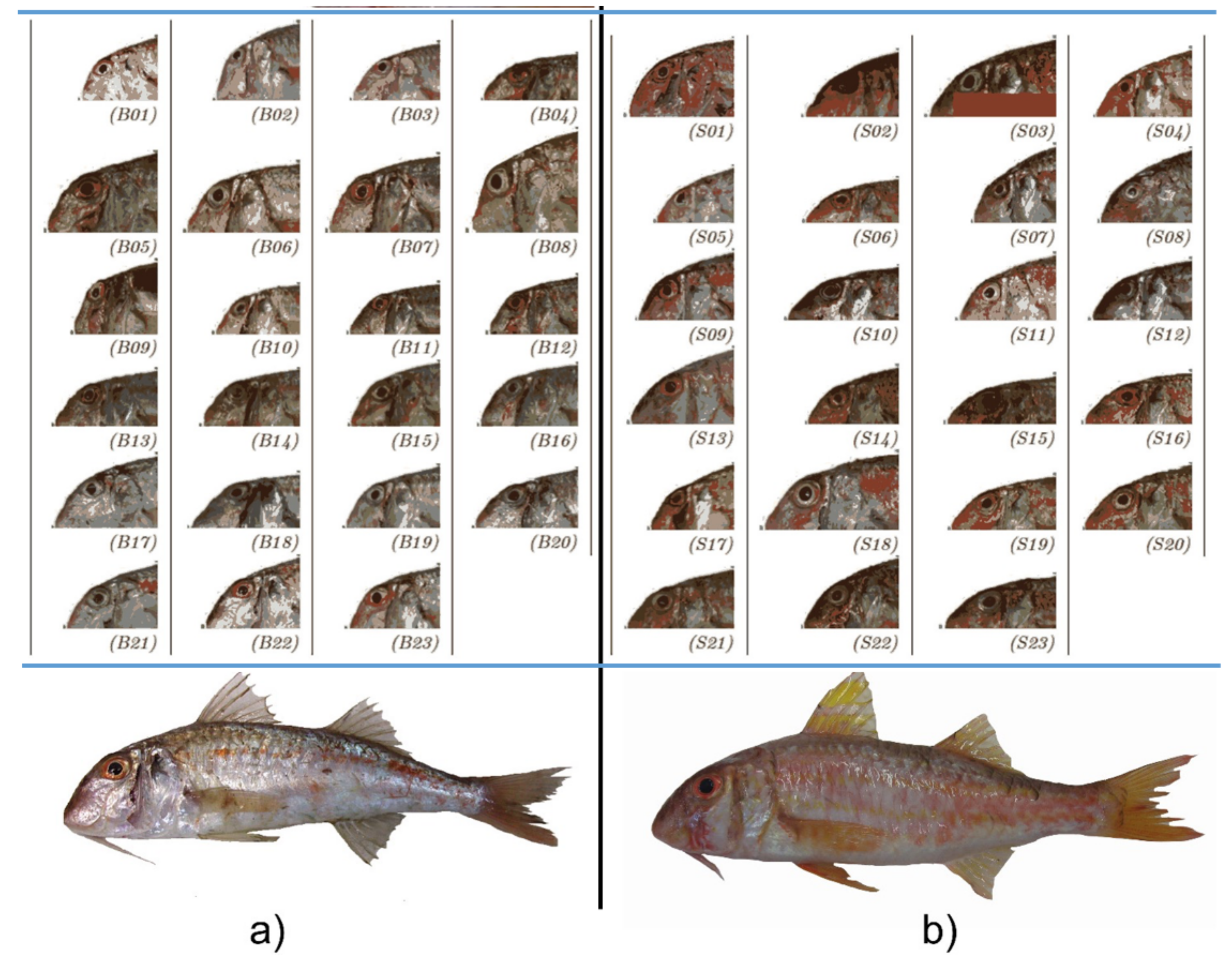
Side-view images of the whole fish were taken in the field with all specimens in the same standardised position and orientation. The fish appear in the center of the image, with the head oriented to the left and the belly facing the bottom of the image. The specimens had different ages and lengths, and the distances from which the pictures were taken were not the same. An expert taxonomist added two points to each image, one to mark the tip of the snout and the other to mark the anterior insertion of the first dorsal fin. Those points indicate the beginning and the end of the contour segments used by taxonomists to identify the mullet’s species. Figure 4 shows, on the bottom, a specimen of each species and, at the top, the profile portion used by the expert to identify the species for all individuals in the database. For this study, we have a data set of 23 images for each species of Red Mullets. The left part is devoted to M. barbatus and the right part to M.surmuletus. Figure 5 shows the head contours of 108 specimens belonging to nine species of Gurnards.
2.3. Open Contour Extraction and Normalization
As the fish were photographed following a certain protocol, they appear in the center of the image, in a horizontal position, with the dorsal fin at the top and the nose oriented to the left. To establish the fragment with relevant information, the expert introduced two marks in all images, one in the snout and the other in the starting point of the dorsal fin, indicating the limits of the contour fragment. These marks are in the background but close to the figure of the fish. Those images are our input data. At that point, the image processing is entirely conventional. Landmark detection can be done by colour. The landmark points are the references that make it possible to automatically crop the original images and thus isolate the profile of interest in a more straightforward and smaller image. In addition, the small size of the new images make the background color more uniform. Contour detection can also be established with a common algorithms presented in the image processing toolbox of MATLAB.
The first step is to convert the region of interest, the ROI, (a colour image) to a grey level in terms of luminance, and then binarize it. There are various methods that can be used to carry out a binarization, but they all depend on a threshold. In our particular case, we employed a global threshold computed using Otsu’s method, which chooses the threshold that minimizes the intraclass variance of black and white pixels [45]. There are more sophisticated methods that can be used to obtain the threshold, but this is the default option used by the function imbinarize in the MATLAB image processing toolbox.
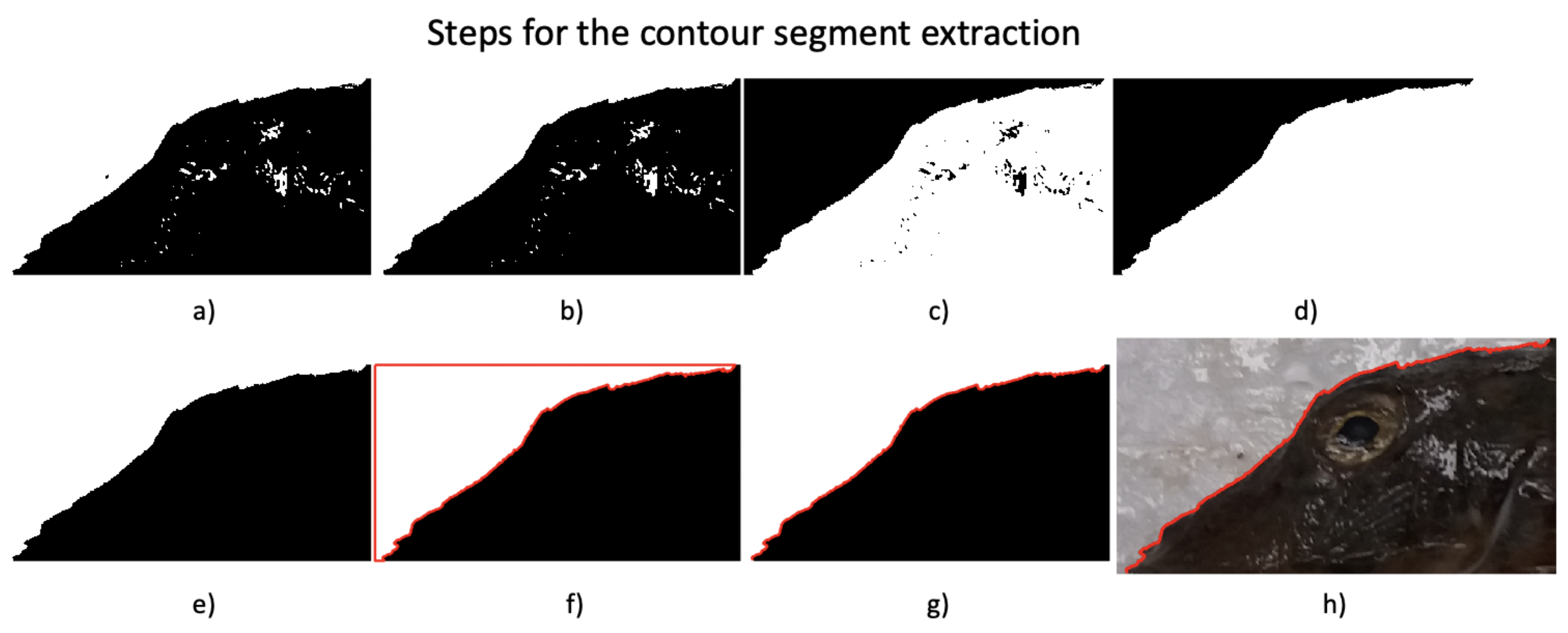
In Figure 6, the sequential steps that are applied in order to obtain the contour segment of interest are shown, for a particular case; in Figure 6a the results of the binarization; in Figure 6b, the black holes in the white region are filled; in Figure 6c, the complement of the previous image; in Figure 6d, the black holes corresponding to the fish are filled; and in Figure 6e, the image is complemented once again to represent the fish in black and the background in white. In Figure 6f, the boundaries of the white region (in red) are found by exploring the image starting from the upper-left pixel and continuing in a downwards direction. In Figure 6g, the image borders are removed to find the contour of interest, which is the final result of the process. Finally, in the sub-image Figure 6h, the obtained result is shown overlapped against the original ROI.
As will be seen, the method developed for this work is very robust to the high-frequency noise that can appear in the determination of contours. Notice that the binary image in Figure 6g can be used as a segmentation template to remove the background, as done in the compositions of Figure 4 and Figure 5. After completing this step, the contour of the specimen i, , is given by its two sequences of horizontal and vertical pixel positions in the cropped image. The origin was taken to be the first point of the open contour, which corresponds to the mark of the nose, and was assigned the (0,0) co-ordinate. The rest of the pixel positions are given relative to this first point and are grouped in the two series . Each contour is represented by a different number of points . Figure 7 shows a cropped image where the contour of interest is delimited by the landmarks and .
Open Contour Normalization
Before the development of the features can be addressed, the open contours must first be normalized. The normalization should be able to compare segments that are represented by a different number of points while also neutralising variations with respect to rotation and scale. Furthermore, care will be taken to ensure that the normalization respects the aspect ratio of the segments. In the case of open contours, the reader can see that the first, () = (), and the last point, (), of the open contour must necessarily differ and, therefore, the reconstruction done with few DFT coefficients could present strong distortions due to the Gibbs phenomenon. However, although the elements and of the sequence differ significantly, the DCT can efficiently approximate the sequence with using few coefficients (L).
As previously demonstrated, the DFT works very well for closed contours because the natural shapes tend to have a smooth variation and, if sampled correctly, the point () is very similar to (), with and being close to and , respectively. The normalization put forward is simple and takes these issues into account. It can be performed following these next two steps:
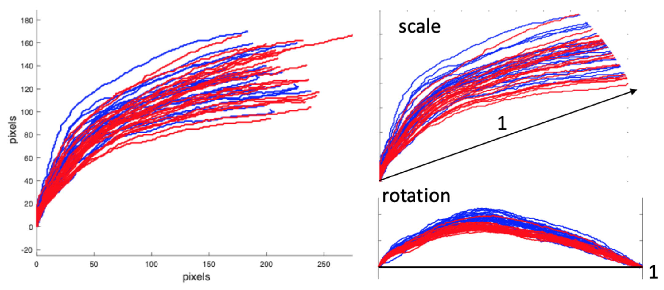
- First, for each open contour, we compute the Euclidean distance between () and (), and the angle that the segment defined by these two points forms with the horizontal. Seen graphically in Figure 7, the points () and () correspond to the landmarks and , respectively. As all the segments begin at , we have:Then, and are used to rotate and re-scale all the contours points according to:After this operation, without changing the aspect ratio, all profiles have been re-scaled and rotated so that they start at point (0,0) and end at point (1,0). Figure 8 separately shows both the scale and scale-and-rotation effects on the original Red Mullet contours. Note in Figure 8 that the relevant information to discriminate the contours is concentrated in (the vertical axis after the rotation) while (the horizontal axis after the rotation) will be very close for all contours and will always go from 0 to 1 in approximately constant increments.
- Second, in order to balance the number of points, the sequence of points is re-sampled so that they all have 256 values. The re-sampling is performed by cubic splines in order to have values at equispaced intervals in the range going from 0 to 1. We call the re-sampled sequence . Finally the contours are represented with a single sequence. In addition, the points and practically take the same value (0), which allows the DFT to be used as well.
2.4. Features Development
Two types of features were developed to feed the classifiers. One is based on the DCT and the other on the DFT. Both take the normalized contour described in the previous section and apply either a DCT or a DFT. In the case of the DCT, we take the first L real coefficients as features . In the case of the DFT, the coefficients are complex and the features are made of the first real parts followed by the first imaginary parts. In that case, as the normalized contour takes real values, the first DFT coefficient is also real and therefore its imaginary part is always zero, and thus is excluded.
From the first N DFT complex coefficients features , are obtained. In addition, for all cases, the vectors of the features are standardised according to the zscore transformation. Thus, in the training step, the means and standard deviations of feature , are computed. The employed features will be . In the test, the averages and standard deviations obtained in the training phase are used to form the features of the segment that is to be classified.
2.5. Extreme Learning Machines, Training and Classification
A single-hidden layer feed-forward neural (SLFN) network is trained as a classifier following the extreme learning machines (ELM) framework [46,47]. The main idea under ELM is that a SLFN network can be trained by randomly assigning both input weights and bias. Proceeding this way, the only parameters to determine in the SLFN network setting are the weights that connect the hidden layer neurons to the outlets (named output weights) and the number H of hidden neurons. This strategy changes the problem of computing the SLFN output weights to a linear problem. The resulting linear over-determined system can be quickly solved using a Moore–Penrose pseudo-inverse in one single step [46,47].
Focusing on our classification problem, each individual i in a set of N is characterized with L features organized in a vector . The matrix of size organizes the features of all N specimens. These individuals are classified into C classes. For each class, there is a vector that indicates with either a 1 or a −1 in the position i whether the individual i belongs (1) or does not belong (−1) to the class c. The vectors are arranged in the matrix of size so that in each row of only one 1 appears. Considering that H is the number of hidden neurons, the input weight matrix will have a size of in which its element is the weight that connects the feature l with the hidden node h. As there are H hidden nodes, there is a vector of bias containing the bias of each node.
Now, considering the individual i, the flow of information into the network can be written as . Taking into account the activation function, which is typically a sigmoid, we have , where applies the sigmoid function to each . Then, when the resulting row vector is multiplied by the output weight matrix of size the resulting row vector will indicate the class to which the individual i belongs. If we group the same equation for all previously classified individuals, ideally we will have the equation:
where is the all-ones vector We define the matrix as:
Then, the ANN formulation can be compactly written as:
Once H is decided, and are randomly selected from a Gaussian distribution function with a mean of zero and a standard deviation of one. The only unknown parameter is . Note that Equation (12) is over-determined. For ELM networks, it is common to choose a number H of hidden nodes lower than the number N of classified cases used for training, that is, . Intuitively, if we see Equation (12) in terms of vectors and of , and respectively, we have , for i going from 1 to C, meaning that for N equations, we have H unknown weights. The output weight matrix , provided that is non singular, is computed by:
where is the Moore–Penrose inverse.
Once , , and are defined, the SLFN can then be used to predict a new individual from its vector of characteristics by applying the following relationship:
where, given a vector , the function finds the maximum value of and returns its position; is the assigned class.
3. Results
3.1. Features Based on the Dct and the Dft. a Comparative Study
3.1.1. Leave-One-Out Cross-Validation
A significant limitation we deal with in this work is the limited number of classified images available for each species used for the training. In the binary classification problem, the two classes are balanced, with 23 individuals in each group. However, in the multi-classification problem, this limitation is more severe, as we have to deal with an even more reduced set of data, which is also unbalanced for the nine groups that need to be classified, meaning that there are different numbers of individuals in each of these groups, as shown in Figure 5.
Despite having these nine classes unbalanced and some of them badly under-represented, the same methodology has been applied in both problems. The leave-one-out cross-validation (LOO-CV) strategy is commonly used to evaluate the performance of the classifier when dealing with small data-sets [48]. This strategy uses a single observation taken from the original data-set to validate the data, while the remaining observations are used for the training phase. This way, the model is built with all the labeled elements except one, which is used for validation. Once the element has been tested, it is added to the group again, and the next element is extracted, repeating the process until all elements have been used for the test. Thus, all the elements are tested against the rest of the known classified elements. The advantage of this method is that all observations are used for both training and validation, and each observation is used for validation exactly once.
3.1.2. LOO-CV Tests
The following tests are intended to determine both the size of the network and the optimal number of characteristics that achieve the best classification rate. The tests that were carried out using features coming from the DFT were then repeated; however, this time using features coming from the DCT, and their results are summarized in Figure 9 and Figure 10.
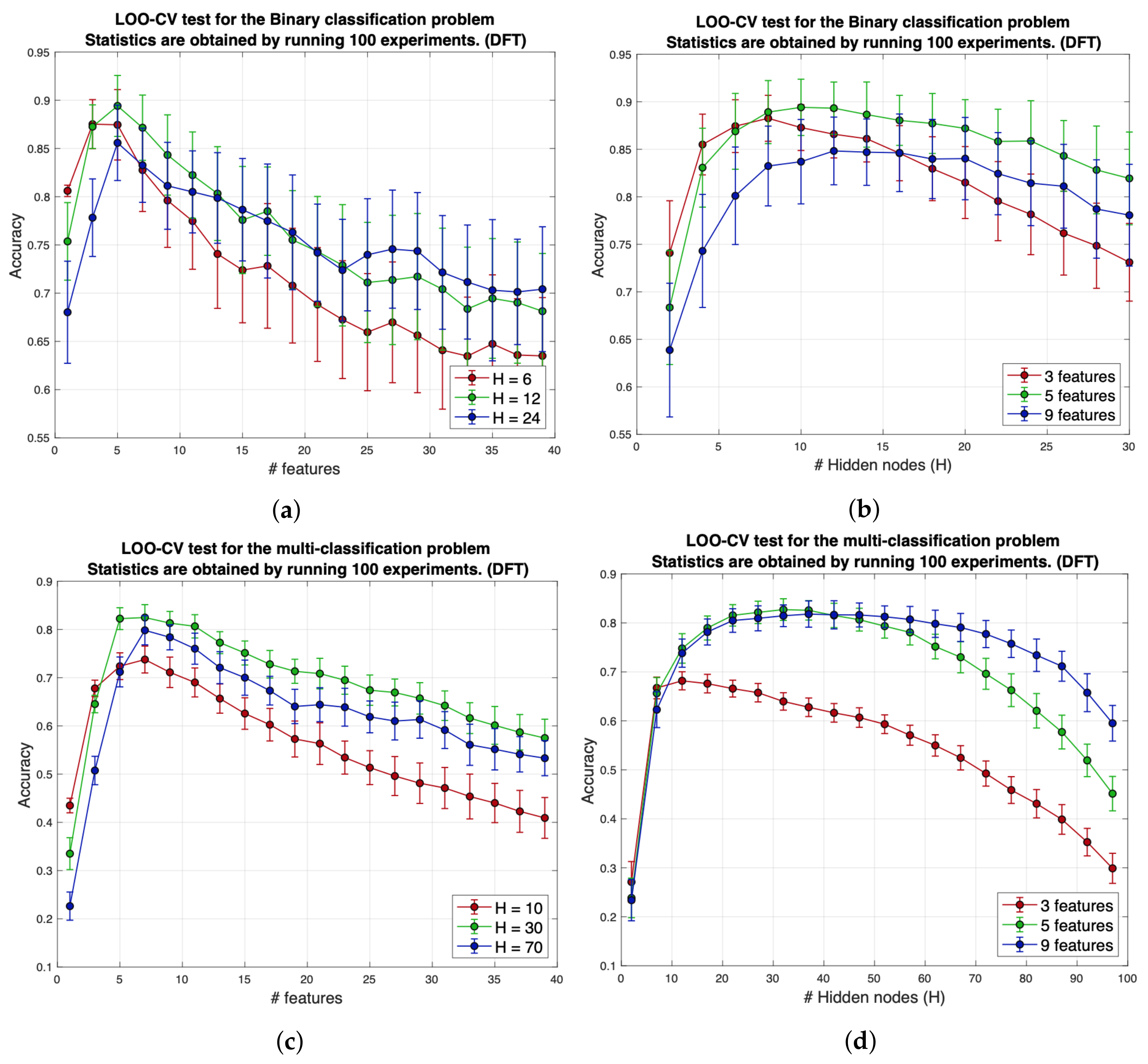
In all these tests, LOO-CV was used to obtain realistic results, and the experiments were repeated 100 times in order to show existing tendencies. Mean values of accuracy, the quotient between the number of correct predictions divided by the number of the predictions done, are represented by color balls and their corresponding standard deviations are shown by vertical lines. The SLFN weights, and , were randomly selected according to a zero-mean Gaussian distribution with a standard deviation of one, where H indicates the number of hidden nodes and L the number of input features. In Figure 9 and Figure 10, N number of transformed coefficients were used. In these figures, note that in the case of the DCT, the number of features (N) is the same as the number of coefficients (L), but in the DFT, instead.
Figure 9 and Figure 10 share the same structure. In both, the Figure 9a,b and Figure 10a,b show the results of the binary classification problem and Figure 9c,d and Figure 10c,d portray the results of the multi-class classification problem. When it comes to the binary problem, the optimal number of DFT-based features is , quite independently of the size of the network (see Figure 9a). The best accuracy values were obtained for H values of around 10 (see Figure 9b).
The best results achieved using the DCT-based features were also obtained for when independently of the size of the network (see Figure 10a). In the same way, the best accuracy results were obtained when (see Figure 10b). In both cases, the best average value for the accuracy was around 0.9 (90%). To obtain the first five features, the first three and five DFT and DCT coefficients were required, respectively. The two encoding alternatives behave in a very similar way, and to decide which one is the best one, the tests need to be refined. Regarding the multi-class classification problem, when using DFT-based features, the best results were attained when .
In this context, the optimum network size increases to values of about (see Figure 9c). Above , there is a wide range of H values for which networks work properly (see Figure 9d). When the DCT is used in this context, the results are very similar, and so from (see Figure 10c) and from (see Figure 10d) there is a wide range of values of L and H for which the networks work correctly. In both cases, independently of the use of DFT/DCT, the average accuracy values are also similar and in the better configurations appear to be slightly above 80%.
From the previous graphs, it is difficult to determine which coding (DFT/DCT) provides the best accuracy, since they behave in a very similar way. In the tests performed below, the number of iterations is incremented to 1000 for a small range of values of H and L near the optimal point of network operation. LOO-CV is always performed. The results are presented in tables indicating the accuracy regarding the average value, standard deviation, and both the maximum and minimum values obtained. The optimal values are represented in bold.
We found that the optimum number of features was 5, independently of which transform (DCT or DFT) was used. Using more than five features reduces the performance of the networks. The only case that differs from the others in the sense of optimal number of features used is that of the binary classification case if the DFT is used, where the best accuracy scores were obtained with three features.
Table 1 shows, for the binary classification problem, a comparative summary of the network accuracy achieved for the best combinations of the DFT (three features) and the DCT (five features) depending on the hidden nodes (H), and Table 2 shows the same information but for the multi-class classification problem, for which the best combination of features is 5 in both the DCT and DFT feature configurations. Table 2 reveals that the best DFT-based configuration exceeds the best DCT-based one by almost two percentage points.
In Table 1, however, it can be seen that the difference between using features derived from the DCT or the DFT is minimal. Regarding the case of the binary classification problem, no combination of features based on the DCT and the DFT was found that improved the results shown in Table 1. In the multi-class classification problem, the aggregation of the five features of each of the best options shown in Table 2 achieved an improvement in the results by almost one percentage point as shown in Table 3.
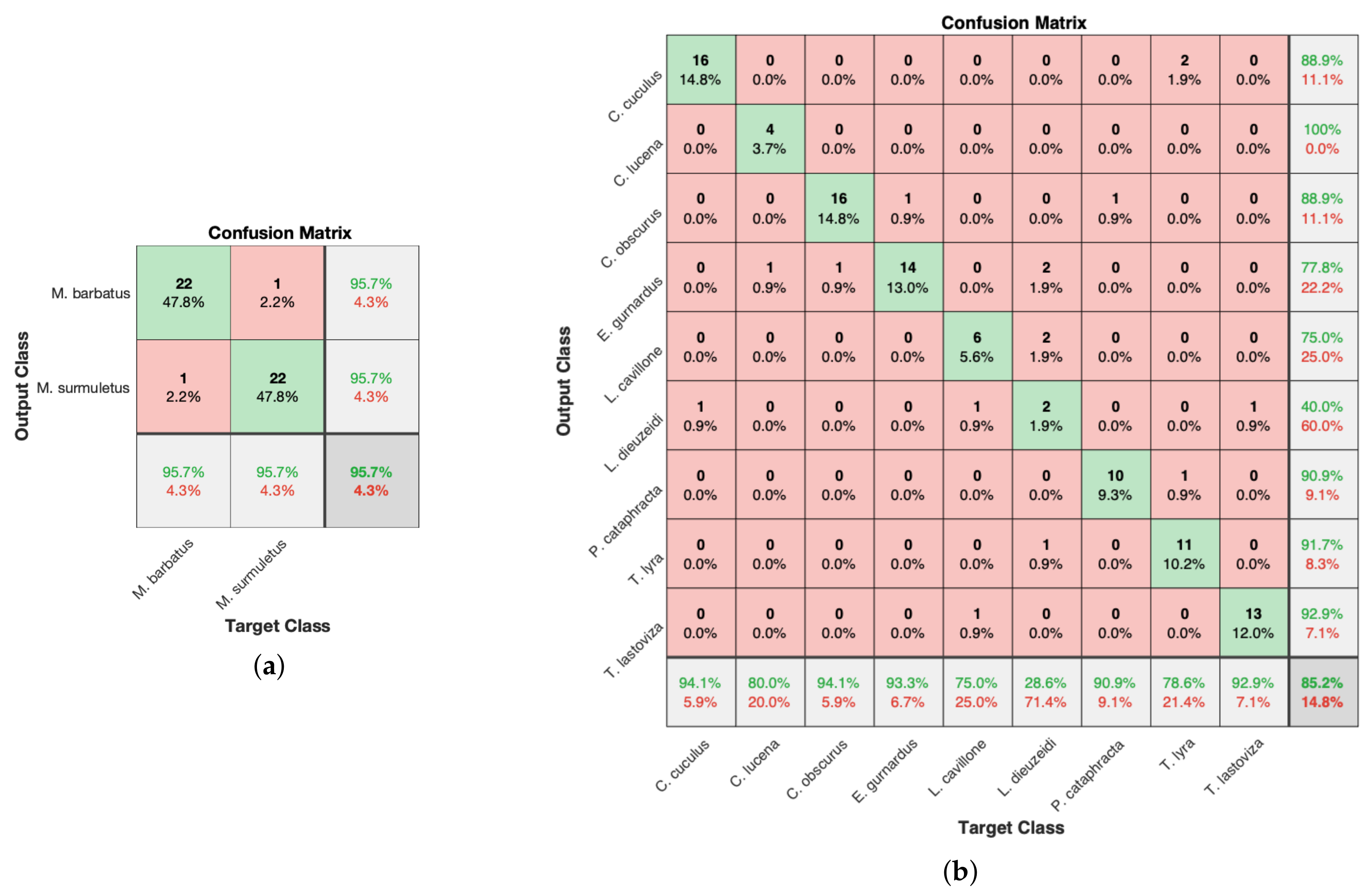
Figure 11 shows the confusion matrices and realizations for both the binary (a) and the multi-class classification (b) problems, respectively. The results were obtained by performing LOO-CV. In both sub-figures, a confusion matrix is shown with a resulting accuracy slightly above the corresponding mean accuracy value. From Figure 11b the correct classification rates of the different classes were acceptably high compared to the ones obtained for the class of Lepidotrigla dieuzeidei.
As explained in this paper, the two points introduced by the specialist were used to segment the region of interest. The introduction of these points unambiguously determines the contour segment used to make the decision. However, this procedure can also be performed automatically. To show that, we conducted the following experiment. We took a set of 50 images, and we randomly took 40 of them to train a faster region-based convolutional network (Faster R-CNN) for object detection, leaving the rest of the images for the test. With this small amount of images, we were able to train a robust model that worked acceptably well. The procedure for training the model was as follows.
The first step was to reduce the images to a size of 384 × 512 pixels. For training, we used the 40 images without marks, and we indicated the region of interest found with the specialist’s marks. This region of interest is a rectangle that is specified with the two extreme points on its main diagonal. We employed the Faster R-CNN object detector provided by MATLAB [49,50]. A Faster R-CNN object detection network is constituted of a feature extraction network followed by two subnetworks.
The feature extraction network is usually a pre-trained CNN. The first subnetwork that supports the feature extraction network is a region proposal network (RPN) devoted to finding the areas in the image where objects are likely to exist. Those areas are known as object proposals. The second subnetwork is dedicated to predicting the class of each object proposal. In the case we are dealing with, for the first network, instead of using a pre-trained CNN as, for instance, the ResNet-50 or the Inception v3, we used a much simpler CNN that has only three convolutional layers from a total of fifteen, that was trained for another problem.
The main characteristics of the structure are summarized in Table 4. The main training options chosen for the Faster R-CNN are ‘MaxEpochs’, ‘MiniBatchSize’ and ‘InitialLearnRate’, which were set to 12, 8, and 5 with a ‘NegativeOverlapRange’ of [0 0.3] and a ‘PositiveOverlapRange’ of [0.6 1]. From these parameters, we note that the ‘MaxEpochs’ specifies the number of epochs, that is, the number of full passes of the training algorithm over the entire training set, and the learning rate that controls the speed of training. The training was performed using the CPU of a MacBook Pro with eight-core Intel i9 processor at 2.4 GHz and 64 GB of RAM running the MATLAB environment on the macOSCatalina 10.15.3 operating system.
Training lasted approximately 3 min. Due to the reasonably fast training time, many random tests on the whole set of images could be performed, and thus the solidity of the approach could be checked. The FasterRCNN object detection network output provides a rectangle by giving two points corresponding to the endpoints of one of its diagonals (specifically the one that goes from the top right to the lower-left point of the rectangle). Some ROI detection results are shown in Figure 12. These points can be used to crop the original image and obtain the ROI, which is practically the same provided by the specialist (although the specialist selects the other diagonal because its endpoints are more near to the segment of interest).
3.2. Regarding Automation of the Whole Process
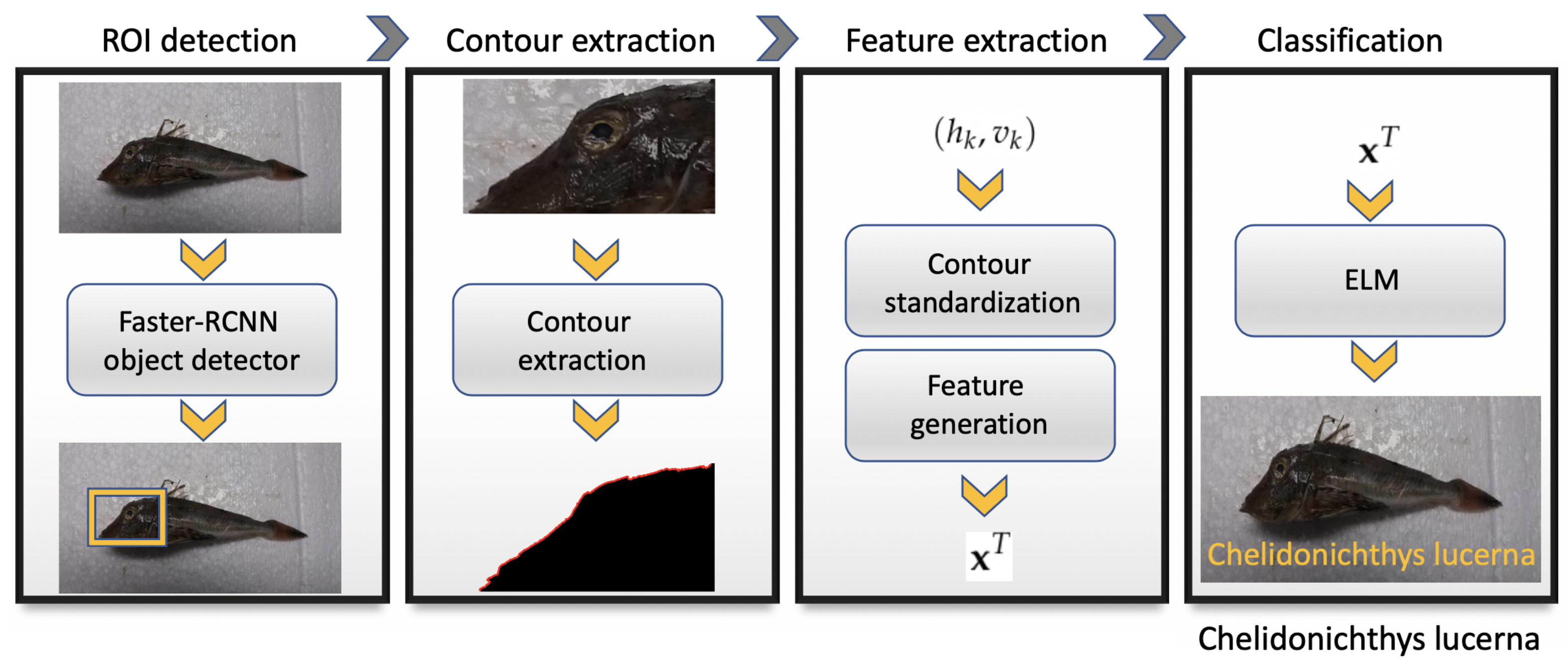
A step that is required to be carried out if the ROI detection is performed without the support of the two points provided by the expert is to re-scale the original image to the FasterRCNN object detection input size, and then, once the ROI is found, it must be mapped onto the original image. This allows the extraction of the ROI from the original image. The following step is to obtain the contour, compute the features, and to introduce them in the ELM network to identify the class of the specimen. The diagram presented in Figure 13 can help to clarify the whole process, which can be described in four stages. The first stage is the ROI detection. This procedure can be supervised or it can be carried out automatically using a Faster-RCNN object detector.
Once the ROI has been determined, the second stage consists of extracting the fish contour segment from this region. The result of stage two is the horizontal and vertical pixel coordinates that describe it in relation to the first contour point, which is taken to be the origin of the coordinate system. The third stage is the ’feature extraction’, in which this sequence of contour points obtained from the previous stage is used as input. These points are standardized by applying a rotation, a re-scaling and a re-sampling by using third-order splines. The result is a single sequence () of 256 values. Then, in the same stage, DCT and DFT are taken on , and we select the first five DCT and DFT coefficients to form the vector of features. In the multi-class classification problem, a features vector containing only 10 real numbers produced the best accuracy results. The vector of features was used in the last stage to add to an already trained ELM of 34 hidden nodes. Finally, the ELM output is the species that the individual belongs to.
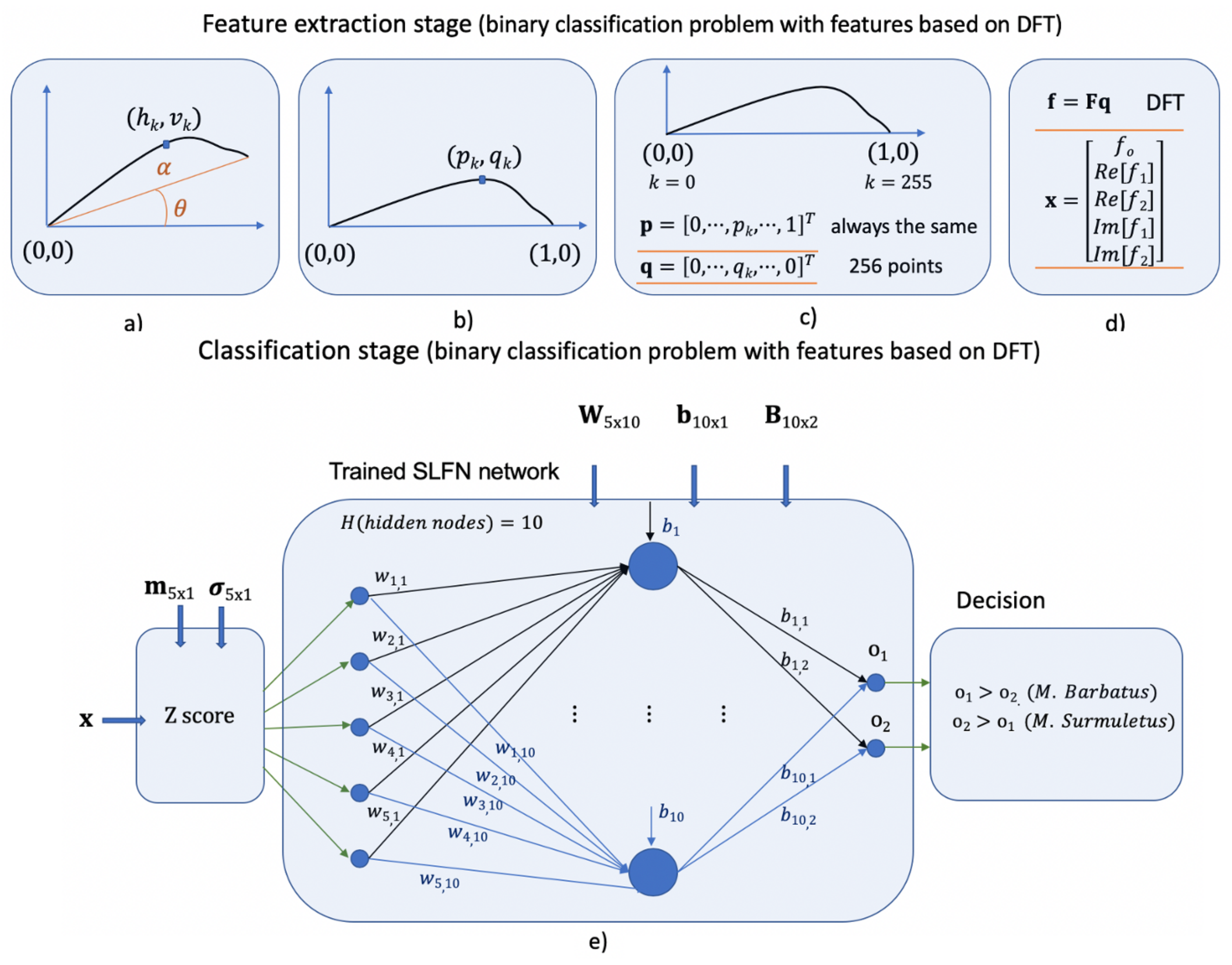
Figure 14 shows the details of a feature extraction stage and of a classification stage corresponding to a model that solves the binary classification problem. It is an SLFN network of 10 hidden nodes trained with features based on the DFT. Figure 14a–c graphically show the steps required to obtain the sequence of 256 points in vector that represent the contour after the standardization, and Figure 14a shows the way to obtain the vector of features. Note than is the Fourier matrix and , the DFT of . In this case, the vector of features has five real elements obtained from the first three Fourier coefficients, as Figure 14e shows the classification stage, which begins with a Z-score standardization, being the vectors and , the means and standard deviations of . The normalized features after the Z-score are the inputs of the SLFN network. , and are the input weights, the bias, and the output weights of the trained SLFN net, respectively. Finally, the decision is taken on the values achieved in the output nodes. This simple architecture reached accuracy values up to 95.65% and, in 1000 LOO-CV experiments a mean accuracy of 89.36% (see the column DFT-3 of Table 1).
Note that, in this case, the fish appears in the images following a standardization, and the problem is not overly complicated. In a random disposition of the objects of interest in the image, one would have to train the model with many more images, using a data augmentation strategy and likely a more complex feature extraction network. Additionally, the substitution of Faster-RCNN by Mask-R CNN [51,52] could be explored to see if the contour segment of interest could even be detected automatically in the ROI directly.
4. Conclusions
In this work, a method was presented that reproduced the procedure that experts perform manually to separate species of fish that exhibit a very similar shape. The technique consists of classifying a fragment from the profile of fish contours. Thus, a way to parameterise open contours was developed based on both the DFT and the DCT transformations, which already allow the discrimination of contour fragments with the use of only five parameters.
The presented approach for the Mullus binary classification case can be compared to the seminal work of Reference [10], which based on handmade measurements of the angle of head contour obtained an 88% correct distinction between both species. The mean accuracy values obtained (89.4%) in this work slightly improved those results. In addition to the difficulty of discriminating between very similar forms, we also had the limitation of having small, unreliably labeled image data sets.
For the second case considered in this work, the multi-class classification problem, it is important to note that there have been no handmade studies carried out that would allow for the comparison of results. The specimens of the database were cataloged at the ICM (Institut de Ciències del Mar) in Barcelona while different types of studies were being conducted. Given the complexity of the problem, the average classification results were close to 80%, which is in line with what trained professionals obtain when they take on the identification and classification task from photographs. If the classification is considered by classes, we observed that the class of Lepidotrigla dieuzeidei was very difficult to classify and thus caused the global accuracy to decrease; however, for the rest of the classes, high correct classification rates were reached.
Our goal was to prove that it is possible to automatically achieve results similar to those obtained by specialists when it comes to classifying very similarly-shaped species of fish. The goal achieved was to automatically classify the images of the specimens in the database into their species. Given the physical similarity between species and the size of the database, this is a difficult objective, which (as we mentioned before) we have overcome with success comparable to that obtained by the expert. The results suggest that we should expect even better results when working with species with more differentiated forms.
For future work, a far more ambitious goal involving government administrations, which must be addressed incrementally, is to computerize the analysis of fish boxes sold at fish markets. In these boxes, fish are stacked in a non-orderly fashion, with the body parts partially hidden but usually with their heads being visible. Thus, the classification of specimens based only on their head contour seems to be indeed an important improvement to be made.
These studies are important as fish markets are beginning to develop projects with the aim of photographing all fish boxes sold, followed by these images being then registered containing information on the labeling, sale prices, and so forth. These large amounts of images can only be processed automatically. As long as the techniques for extracting information from images continues improving, we will be able to obtain a gradually deeper understanding on the exploitation of marine resources. This work is a pioneer in the classification of biological forms through contour segments.
In this paper, the identification of the contour fragments was made with the help of marks. In this way, we were sure to deal with the fragment used by the experts. In the type of images used, the marks were located in easily identifiable positions and, even though this was not the purpose of this work, it was even shown in a prior subsection that these are not entirely necessary. Although this technique has been developed for a certain type of image, the capacity of representing contour segments between landmarks with very few parameters could be interesting and further explored in different contexts and applications.
The human visual system is particularly sensitive to the contour of a shape, and curves constitute an essential information element when it comes to image analysis, classification and pattern recognition, which are vital tasks that humans carry out on a daily basis. The necessity to quantify this visual information continues in present challenges, as was the case for this work, in which the relevant information that led to a good classification rate was concentrated only on a specific fragment of the silhouette instead of the whole contour. In this work, we have the additional restriction of having little data available to use for training purposes, which imposes a classic machine learning work-flow, typically seen when dealing with small datasets.
In spite of that, this study suggested that the combination of machine learning (ML) and deep learning (DL) techniques can provide compelling solutions. On the one hand, through ML, we can (1) handle small datasets and (2) maintain the understanding of the problem. At the same time, DL reached milestones in image processing that were previously difficult to obtain, such as the identification of the ROI where the contour fragment is located. Finally, the ELM-based classifiers provided excellent results at low computational and time costs, which allowed for complete statistical tests.
Author Contributions
Conceptualization, P.M.-P. and A.L.; methodology, P.M.-P., A.M., and A.L.; software, P.M.-P. and A.M.; validation, P.M.-P., A.M., and A.L.; formal analysis, P.M.-P., and A.L.; investigation, P.M.-P. and A.L.; resources, A.L.; writing, original draft preparation, P.M.-P. and A.L.; writing, review and editing, P.M.-P., A.M., and A.L.; supervision, P.M.-P. and A.L.; funding acquisition, A.L. All authors read and agreed to the published version of the manuscript.
Funding
This work has been partially supported by the Spanish Government projects PHENOFISH with references: CTM2015-69126-C2-2-R and Catalan Government project PESCAT, with reference ARP029/18/00003.
Acknowledgments
We thank Marta Blanco and Marc Balcells from SAP-ICATMAR for images of commercial fish that were made available to us.
Conflicts of Interest
The authors declare no conflict of interest.
References
- Azzurro, E.; Tuset, V.M.; Lombarte, A.; Maynou, F.; Simberloff, D.; Rodríguez-Pérez, A.; Solé, R.V. External morphology explains the success of biological invasions. Ecol. Lett. 2014, 17, 1455–1463. [Google Scholar] [CrossRef] [PubMed]
- Stergiou, K.; Petrakis, G.; Papaconstantinou, C. The Mullidae (Mullus barbatus, M. surmuletus) fishery in Greek waters, 1964–1986. In FAO Fisheries Report (FAO); FAO: Rome, Italy, 1992. [Google Scholar]
- Renones, O.; Massuti, E.; Morales-Nin, B. Life history of the red mullet Mullus surmuletus from the bottom-trawl fishery off the Island of Majorca (north-west Mediterranean). Mar. Biol. 1995, 123, 411–419. [Google Scholar] [CrossRef]
- Bautista-Vega, A.; Letourneur, Y.; Harmelin-Vivien, M.; Salen-Picard, C. Difference in diet and size-related trophic level in two sympatric fish species, the red mullets Mullus barbatus and Mullus surmuletus, in the Gulf of Lions (north-west Mediterranean Sea). J. Fish Biol. 2008, 73, 2402–2420. [Google Scholar] [CrossRef]
- Cresson, P.; Bouchoucha, M.; Miralles, F.; Elleboode, R.; Mahe, K.; Marusczak, N.; Thebault, H.; Cossa, D. Are red mullet efficient as bio-indicators of mercury contamination? A case study from the French Mediterranean. Mar. Pollut. Bull. 2015, 91, 191–199. [Google Scholar] [CrossRef] [Green Version]
- Golani, D.; Galil, B. Trophic relationships of colonizing and indigenous goatfishes (Mullidae) in the eastern Mediterranean with special emphasis on decapod crustaceans. Hydrobiologia 1991, 218, 27–33. [Google Scholar] [CrossRef]
- Labropoulou, M.; Eleftheriou, A. The foraging ecology of two pairs of congeneric demersal fish species: Importance of morphological characteristics in prey selection. J. Fish Biol. 1997, 50, 324–340. [Google Scholar] [CrossRef]
- Lombarte, A.; Recasens, L.; González, M.; de Sola, L.G. Spatial segregation of two species of Mullidae (Mullus surmuletus and M. barbatus) in relation to habitat. Mar. Ecol. Prog. Ser. 2000, 206, 239–249. [Google Scholar] [CrossRef]
- Maravelias, C.D.; Tsitsika, E.V.; Papaconstantinou, C. Environmental influences on the spatial distribution of European hake (Merluccius merluccius) and red mullet (Mullus barbatus) in the Mediterranean. Ecol. Res. 2007, 22, 678–685. [Google Scholar] [CrossRef]
- Bougis, P. Recherches Biométriques sur les Rougets,‘Mullus barbatus’ L. et‘Mullus surmuletus’ L...; Centre National de la Recherche Scientifique: Paris, France, 1952. [Google Scholar]
- Tortonese, E.; di Entomologia, A.N.I.; Italiana, U.Z. Osteichthyes (Pesci Ossei): Parte Seconda; Edizioni Calderini Bologna: Bologna, France, 1975. [Google Scholar]
- Lombarte, A.; Aguirre, H. Quantitative differences in the chemoreceptor systems in the barbels of two species of Mullidae (Mullus surmuletus and M. barbatus) with different bottom habitats. Mar. Ecol. Prog. Ser. 1997, 150, 57–64. [Google Scholar] [CrossRef] [Green Version]
- Aguirre, H. Presence of dentition in the premaxilla of juvenile Mullus barbatus and M. surmuletus. J. Fish Biol. 1997, 51, 1186–1191. [Google Scholar] [CrossRef]
- Aguirre, H.; Lombarte, A. Ecomorphological comparisons of sagittae in Mullus barbatus and M. surmuletus. J. Fish Biol. 1999, 55, 105–114. [Google Scholar] [CrossRef]
- Hureau, J.; Bauchot, M.; Nielsen, J.; Tortonese, E. Fishes of the North-Eastern Atlantic and the Mediterranean; Unesco: Paris, France, 1986; Volume 3. [Google Scholar]
- Kuhl, F.P.; Giardina, C.R. Elliptic Fourier features of a closed contour. Comput. Graph. Image Process. 1982, 18, 236–258. [Google Scholar] [CrossRef]
- El-ghazal, A.; Basir, O.; Belkasim, S. Farthest point distance: A new shape signature for Fourier descriptors. Signal Process. Image Commun. 2009, 24, 572–586. [Google Scholar] [CrossRef]
- Persoon, E.; Fu, K.S. Shape discrimination using Fourier descriptors. IEEE Trans. Syst. Man Cybern. 1977, 7, 170–179. [Google Scholar] [CrossRef]
- Tracey, S.R.; Lyle, J.M.; Duhamel, G. Application of elliptical Fourier analysis of otolith form as a tool for stock identification. Fish. Res. 2006, 77, 138–147. [Google Scholar] [CrossRef]
- Lestrel, P.E. Fourier Descriptors and Their Applications in Biology; Cambridge University Press: Cambridge, UK, 2008. [Google Scholar]
- Mokhtarian, F.; Abbasi, S.; Kittler, J. Robust and E cient Shape Indexing through Curvature Scale Space. In Proceedings of the 1996 British Machine and Vision Conference BMVC, Edinburgh, UK, 9–12 September 1996; Volume 96. [Google Scholar]
- Dudek, G.; Tsotsos, J.K. Shape representation and recognition from multiscale curvature. Comput. Vis. Image Underst. 1997, 68, 170–189. [Google Scholar] [CrossRef] [Green Version]
- Mokhtarian, F.; Bober, M. Curvature Scale Space Representation: Theory, Applications, and MPEG-7 Standardization; Springer Science & Business Media: Berlin/Heidelberg, Germany, 2013; Volume 25. [Google Scholar]
- Parisi-Baradad, V.; Lombarte, A.; García-Ladona, E.; Cabestany, J.; Piera, J.; Chic, O. Otolith shape contour analysis using affine transformation invariant wavelet transforms and curvature scale space representation. Mar. Freshw. Res. 2005, 56, 795–804. [Google Scholar] [CrossRef]
- Gibbs, J.W. Fourier’s series. Nature 1899, 59, 606. [Google Scholar] [CrossRef]
- Toubin, M.; Dumont, C.; Verrecchia, E.P.; Laligant, O.; Diou, A.; Truchetet, F.; Abidi, M. Multi-scale analysis of shell growth increments using wavelet transform. Comput. Geosci. 1999, 25, 877–885. [Google Scholar] [CrossRef] [Green Version]
- Allen, E.G. New approaches to Fourier analysis of ammonoid sutures and other complex, open curves. Paleobiology 2006, 32, 299–315. [Google Scholar] [CrossRef]
- Yang, C.; Tiebe, O.; Shirahama, K.; Łukasik, E.; Grzegorzek, M. Evaluating contour segment descriptors. Mach. Vis. Appl. 2017, 28, 373–391. [Google Scholar] [CrossRef]
- Dommergues, C.H.; Dommergues, J.L.; Verrecchia, E.P. The discrete cosine transform, a Fourier-related method for morphometric analysis of open contours. Math. Geol. 2007, 39, 749–763. [Google Scholar] [CrossRef] [Green Version]
- Wilczek, J.; Monna, F.; Barral, P.; Burlet, L.; Chateau, C.; Navarro, N. Morphometrics of Second Iron Age ceramics–strengths, weaknesses, and comparison with traditional typology. J. Archaeol. Sci. 2014, 50, 39–50. [Google Scholar] [CrossRef]
- Stefanini, M.I.; Carmona, P.M.; Iglesias, P.P.; Soto, E.M.; Soto, I.M. Differential Rates of Male Genital Evolution in Sibling Species of Drosophila. Evol. Biol. 2018, 45, 211–222. [Google Scholar] [CrossRef]
- Ahmed, N.; Natarajan, T.; Rao, K.R. Discrete cosine transform. IEEE Trans. Comput. 1974, 100, 90–93. [Google Scholar] [CrossRef]
- Kou, W.; Mark, J.W. A new look at DCT-type transforms. IEEE Trans. Acoust. Speech Signal Process. 1989, 37, 1899–1908. [Google Scholar] [CrossRef]
- Martucci, S. Symmetric convolution and the discrete sine and cosine transforms. IEEE Trans. Signal Process. 1994, 42, 1038–1051. [Google Scholar] [CrossRef]
- Strang, G. The discrete cosine transform. SIAM Rev. 1999, 41, 135–147. [Google Scholar] [CrossRef]
- Suresh, K.; Sreenivas, T. Linear filtering in DCT IV/DST IV and MDCT/MDST domain. Signal Process. 2009, 89, 1081–1089. [Google Scholar] [CrossRef]
- Britanak, V.; Yip, P.C.; Rao, K.R. Discrete Cosine and Sine Transforms: General Properties, Fast Algorithms and Integer Approximations; Academic Press: Cambridge, MA, USA, 2010. [Google Scholar]
- Tsitsas, N.L. On block matrices associated with discrete trigonometric transforms and their use in the theory of wave propagation. J. Comput. Math. 2010, 28, 864–878. [Google Scholar] [CrossRef]
- Ito, I.; Kiya, H. A computing method for linear convolution in the DCT domain. In Proceedings of the 2011 19th European Signal Processing Conference, Barcelona, Spain, 29 August–2 September 2011; pp. 323–327. [Google Scholar]
- Rao, K.R.; Yip, P. Discrete Cosine Transform: Algorithms, Advantages, Applications; Academic Press: Cambridge, MA, USA, 2014. [Google Scholar]
- Wang, Z. Fast algorithms for the discrete W transform and for the discrete Fourier transform. IEEE Trans. Acoust. Speech Signal Process. 1984, 32, 803–816. [Google Scholar] [CrossRef]
- Roma, N.; Sousa, L. A tutorial overview on the properties of the discrete cosine transform for encoded image and video processing. Signal Process. 2011, 91, 2443–2464. [Google Scholar] [CrossRef]
- Massutí, E.; Reñones, O. Demersal resource assemblages in the trawl fishing grounds off the Balearic Islands (western Mediterranean). Sci. Mar. 2005, 69, 167–181. [Google Scholar] [CrossRef] [Green Version]
- Balcells, M.; Fernández-Arcaya, U.; Lombarte, A.; Ramon, M.; Abelló, P.; Mecho, A.; Company, J.; Recasens, L. Effect of a small-scale fishing closure area on the demersal community in the NW Mediterranean Sea. In Rapports et Procès-Verbaux des Réunions de la Commission Internationale pour l’Exploration Scientifique de la Mer Méditerranée; Mediterranean Science Commission: Kiel, Germany, 2016; pp. 41–517. [Google Scholar]
- Otsu, N. A threshold selection method from gray-level histograms. IEEE Trans. Syst. Man Cybern. 1979, 9, 62–66. [Google Scholar] [CrossRef] [Green Version]
- Huang, G.B.; Chen, L.; Siew, C.K. Universal approximation using incremental constructive feedforward networks with random hidden nodes. IEEE Trans. Neural Netw. 2006, 17, 879–892. [Google Scholar] [CrossRef] [Green Version]
- Huang, G.B.; Zhu, Q.Y.; Siew, C.K. Extreme learning machine: Theory and applications. Neurocomputing 2006, 70, 489–501. [Google Scholar] [CrossRef]
- Vapnik, V. The Nature of Statistical Learning Theory; Springer Science & Business Media: Berlin/Heidelberg, Germany, 2013. [Google Scholar]
- Ren, S.; He, K.; Girshick, R.; Sun, J. Faster r-cnn: Towards real-time object detection with region proposal networks. In Proceedings of the Advances in Neural Information Processing Systems, Montreal, QC, Canada, 7–12 December 2015; pp. 91–99. [Google Scholar]
- Ren, S.; He, K.; Girshick, R.; Sun, J. Faster R-CNN: Towards Real-Time Object Detection with Region Proposal Networks. IEEE Trans. Pattern Anal. Mach. Intell. 2017, 39, 1137. [Google Scholar] [CrossRef] [PubMed] [Green Version]
- He, K.; Gkioxari, G.; Dollár, P.; Girshick, R. Mask r-cnn. In Proceedings of the IEEE International Conference on Computer Vision, Venice, Italy, 22–29 October 2017; pp. 2961–2969. [Google Scholar]
- Álvarez-Ellacuría, A.; Palmer, M.; Catalán, I.A.; Lisani, J.L. Image-based, unsupervised estimation of fish size from commercial landings using deep learning. ICES J. Mar. Sci. 2019. [Google Scholar] [CrossRef]
Figure 1.
A presentation of the traditional mixture that is made by fishermen in the Catalan coast: (a) red mullets, and (b) gurnards.
Figure 1.
A presentation of the traditional mixture that is made by fishermen in the Catalan coast: (a) red mullets, and (b) gurnards.
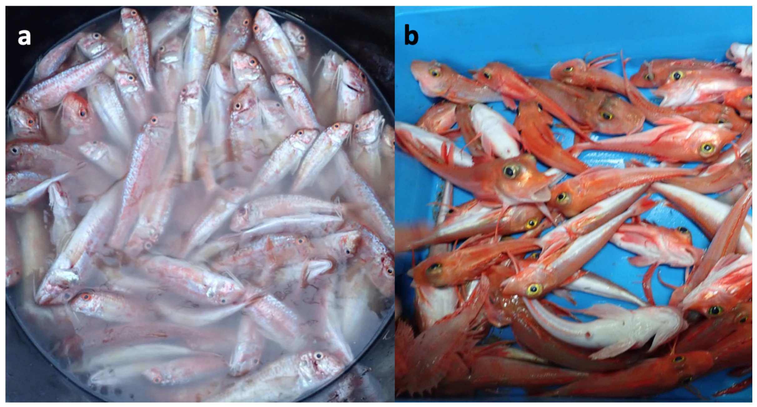
Figure 2.
The four possible sequence extensions in discrete trigonometric transforms (DTTs) depending on the point of symmetry (POS) and the type. HS, HA, WS, and WA stand for half sample-symmetry, half sample anti-symmetry, whole sample-symmetry and whole sample anti-symmetry, respectively.
Figure 2.
The four possible sequence extensions in discrete trigonometric transforms (DTTs) depending on the point of symmetry (POS) and the type. HS, HA, WS, and WA stand for half sample-symmetry, half sample anti-symmetry, whole sample-symmetry and whole sample anti-symmetry, respectively.

Figure 3.
(a) Implicit extensions outside the main range for discrete cosine transform (DCT) formulations -I, -II, -V and -VI. The main sequence is in bold. (b) Discrete Fourier transform (DFT) implicit extensions for the same sequence. (c) Reconstruction of a set of 32 original points (squares) using four real DCT-II coefficients (circles) and seven complex DFT coefficients and (triangles). Note that are the complex conjugates of , respectively.
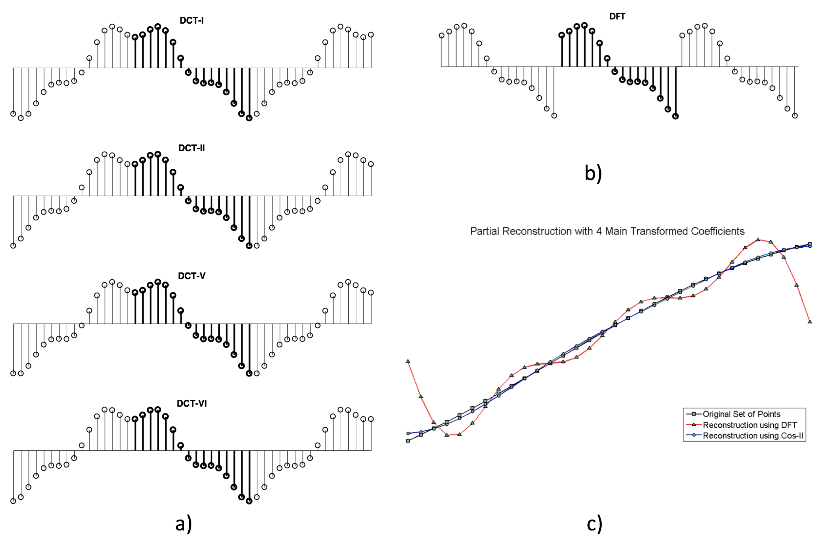
Figure 4.
(a) Mullus barbatus and (b) Mullus surmuletus specimens in the database. The images on the top show the profile of interest according to taxonomist criteria. The specimens are identified with the letter B/S plus a number.
Figure 4.
(a) Mullus barbatus and (b) Mullus surmuletus specimens in the database. The images on the top show the profile of interest according to taxonomist criteria. The specimens are identified with the letter B/S plus a number.

Figure 5.
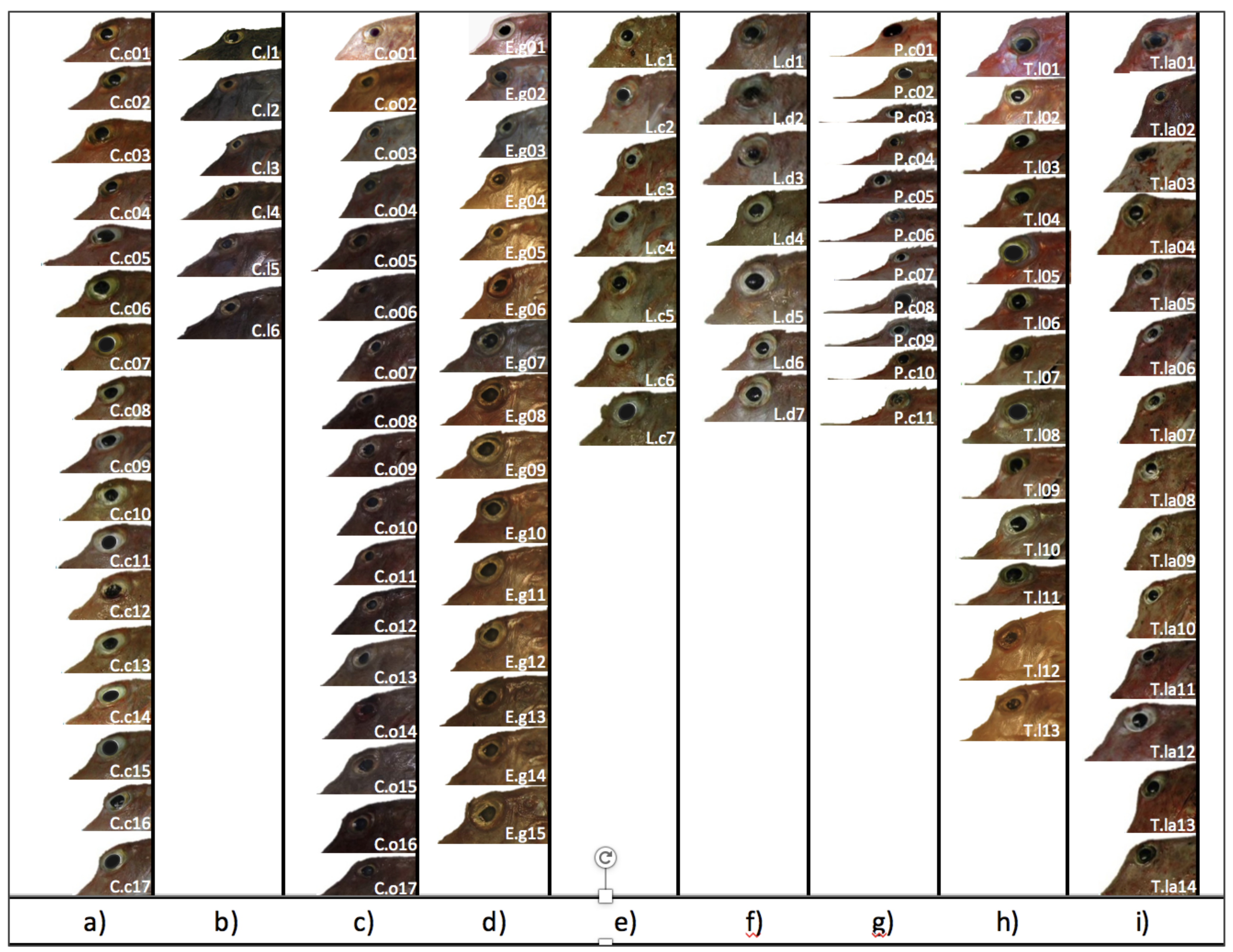
The images show the profiles of interest of the specimens in the database according to taxonomist criteria. (a) Chelidonichthys cuculus (C.c#), (b) Chelidonichthys lucerna (C.l#), (c) Chelidonichthys obscurus (C.o#), (d) Eutrigla gurnardus (E.g#), (e) Lepidotrigla cavillone (L.c#), (f) Lepidotrigla dieuzeidei (L.d#), (g) Peristedion cataphractum (P.c#), (h) Trigla lyra (T.l#), and (i) Trigloporus lastoviza (T.l#).
Figure 5.
The images show the profiles of interest of the specimens in the database according to taxonomist criteria. (a) Chelidonichthys cuculus (C.c#), (b) Chelidonichthys lucerna (C.l#), (c) Chelidonichthys obscurus (C.o#), (d) Eutrigla gurnardus (E.g#), (e) Lepidotrigla cavillone (L.c#), (f) Lepidotrigla dieuzeidei (L.d#), (g) Peristedion cataphractum (P.c#), (h) Trigla lyra (T.l#), and (i) Trigloporus lastoviza (T.l#).

Figure 6.
Steps for the contour segment extraction. In (a), binarization; in (b–e), the steps to fill the gaps in the background and in the fish regions; in (f), the boundary detection of the white region; and in (g), the contour of interest found after removing the image borders.
Figure 6.
Steps for the contour segment extraction. In (a), binarization; in (b–e), the steps to fill the gaps in the background and in the fish regions; in (f), the boundary detection of the white region; and in (g), the contour of interest found after removing the image borders.

Figure 7.
Fragment of interest of the fish delimited by landmarks and .
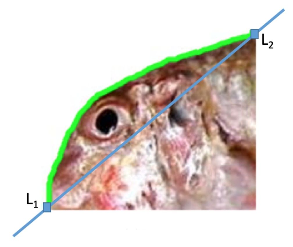
Figure 8.
Representation of the scale and scale-&-rotation effects on the original Red Mullet contours. These changes are performed during the contour normalization process.
Figure 8.
Representation of the scale and scale-&-rotation effects on the original Red Mullet contours. These changes are performed during the contour normalization process.

Figure 9.
The accuracy obtained by training a single-hidden layer feed-forward neural (SLFN) with the DFT-based features. Leave-one-out cross-validation (LOO-CV).
Figure 9.
The accuracy obtained by training a single-hidden layer feed-forward neural (SLFN) with the DFT-based features. Leave-one-out cross-validation (LOO-CV).

Figure 10.
The accuracy obtained by training SLFN with the DCT-based features.

Figure 11.
(a) The confusion matrix of binary-classification realization with an accuracy value of 95.7%. The results were obtained by performing LOO-CV using five features based on the DFT with a SLFN of 10 hidden nodes. The mean accuracy value after performing 1000 LOO-CV iterations was 89.3%. (b) The confusion matrix of multi-class classification realization with 85.2% accuracy. The results were obtained by performing LOO-CV using five features based on the DCT plus five more based on the DFT, with an SLFN of 30 hidden nodes. The mean accuracy value after performing 1000 LOO-CV iterations maintaining the same SLFN size was 83.15%.

Figure 12.
Example of the detection results performed on the test images using the trained faster region-based convolutional network (Faster R-CNN) object detector. The obtained ROI is shown in yellow.
Figure 12.
Example of the detection results performed on the test images using the trained faster region-based convolutional network (Faster R-CNN) object detector. The obtained ROI is shown in yellow.
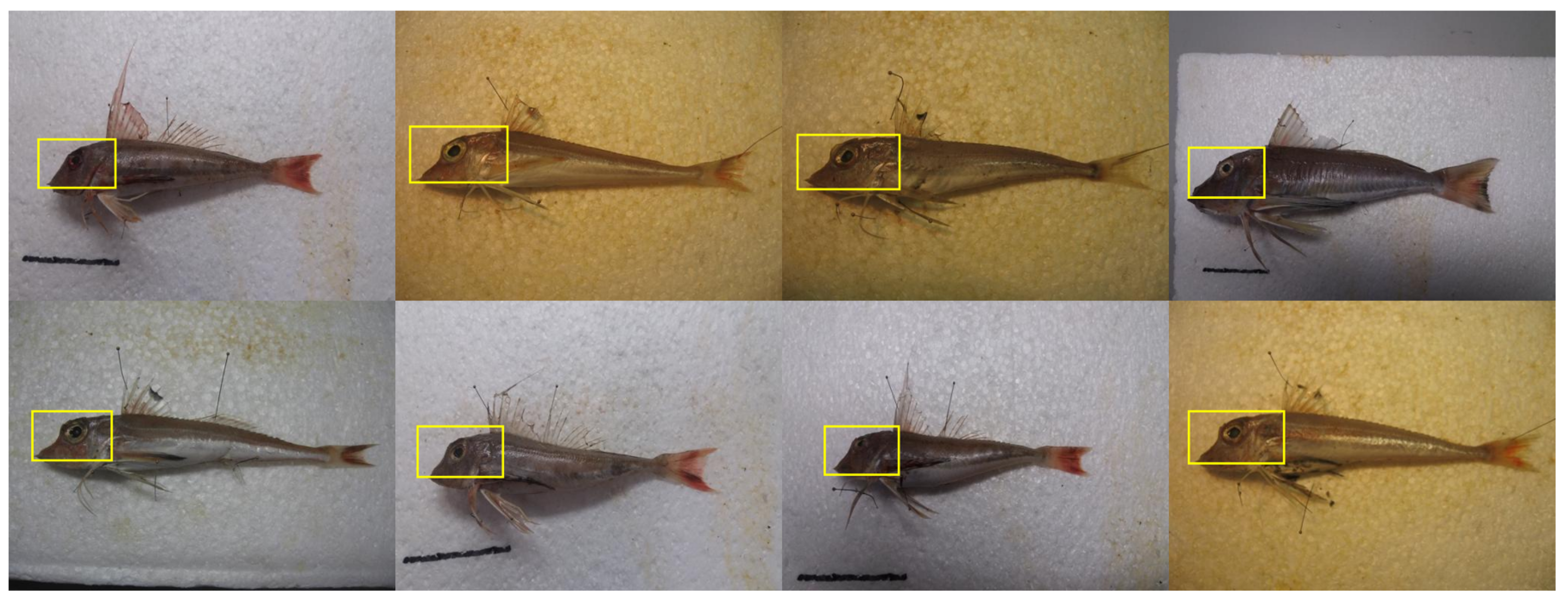
Figure 13.
Simplified block diagram of the process chain when the ROI detection is done automatically.
Figure 13.
Simplified block diagram of the process chain when the ROI detection is done automatically.

Figure 14.
Detail at the parameter level of the feature extraction and classification stages of the binary classification solution working with features based on DFT. (a–c) show the steps required to obtain the vector from the contour, and (d) shows the way to obtain the vector from . In (e), the classification stage is shown with the parameters that interact in each step. The matrices and vectors show their dimensions in a subscript (in order to check the coherence of the operations involved). In the classification stage, three parts, the Z-score normalization, an LSFN network of 10 hidden nodes, and the decision rule, are employed.


Table 1.
The binary classification problem. A comparative summary of the network accuracy obtained for the best combinations of the DCT (five features) and the DFT (three features) depending on the hidden nodes used. The LOO-CV was performed and the experiments were repeated 1000 times. For each feature set, there is an optimum number of hidden nodes that provide the best results. In the table the bests accuracy results are highlighted in bold.
| Binary-Class Classification Accuracy (LOO-CV 1000 Iterations) | ||||||||
|---|---|---|---|---|---|---|---|---|
| Hidden | DCT-5 | DFT-3 | ||||||
| Nodes | mean | std | max | min | mean | std | max | min |
| 7 | 88.44 | 0.031 | 95.65 | 78.26 | 88.46 | 0.032 | 95.65 | 76.09 |
| 8 | 89.09 | 0.031 | 95.65 | 78.26 | 89.09 | 0.030 | 95.65 | 78.26 |
| 9 | 89.37 | 0.030 | 97.83 | 80.44 | 89.29 | 0.031 | 95.65 | 76.09 |
| 10 | 89.30 | 0.031 | 95.65 | 78.26 | 89.36 | 0.028 | 95.65 | 80.44 |
| 11 | 89.34 | 0.029 | 95.65 | 80.44 | 89.19 | 0.030 | 95.65 | 78.26 |
| 12 | 89.33 | 0.031 | 95.65 | 80.44 | 89.20 | 0.030 | 95.65 | 78.26 |
| 13 | 89.04 | 0.031 | 95.65 | 78.26 | 89.10 | 0.030 | 95.65 | 80.44 |
| 14 | 88.76 | 0.032 | 95.65 | 78.26 | 88.64 | 0.032 | 95.65 | 78.26 |
| 15 | 88.80 | 0.031 | 95.65 | 78.26 | 88.57 | 0.031 | 95.65 | 76.09 |
| 16 | 88.40 | 0.032 | 95.65 | 78.26 | 88.14 | 0.033 | 95.65 | 73.91 |
| 17 | 88.05 | 0.033 | 95.65 | 78.26 | 87.92 | 0.033 | 95.65 | 76.09 |
Table 2.
The multi-class classification problem. Comparative summary of the network accuracy obtained for the best combinations of the DCT (five features) and the DFT (five features) depending on the hidden nodes used. For each feature set, there is an optimum number of hidden nodes providing the best results. In the table the bests accuracy results are highlighted in bold. The LOO-CV was performed and the experiments were repeated 1000 times.
| Multi-Class Classification Accuracy (LOO-CV 1000 Iterations) | ||||||||
|---|---|---|---|---|---|---|---|---|
| Hidden | DCT-5 | DFT-5 | ||||||
| Nodes | mean | std | max | min | mean | std | max | min |
| 5 | 72.66 | 0.024 | 79.63 | 64.82 | 56.78 | 0.035 | 66.67 | 44.44 |
| 10 | 72.66 | 0.024 | 79.63 | 64.82 | 72.29 | 0.029 | 81.48 | 63.89 |
| 15 | 76.66 | 0.023 | 84.26 | 68.52 | 77.78 | 0.024 | 85.19 | 69.44 |
| 20 | 78.62 | 0.022 | 85.19 | 72.22 | 80.52 | 0.024 | 88.89 | 72.22 |
| 25 | 79.84 | 0.023 | 87.04 | 72.22 | 82.04 | 0.021 | 87.96 | 74.07 |
| 30 | 80.42 | 0.023 | 87.04 | 72.22 | 82.59 | 0.021 | 88.89 | 75.00 |
| 35 | 80.64 | 0.022 | 87.04 | 73.19 | 82.49 | 0.022 | 87.96 | 75.00 |
| 40 | 80.54 | 0.023 | 87.96 | 73.19 | 81.94 | 0.022 | 88.89 | 74.07 |
| 45 | 80.00 | 0.024 | 87.04 | 72.22 | 81.18 | 0.029 | 87.04 | 74.07 |
| 50 | 79.38 | 0.025 | 87.04 | 71.30 | 79.79 | 0.024 | 86.11 | 72.22 |
| 55 | 78.18 | 0.025 | 87.04 | 69.44 | 78.15 | 0.025 | 85.19 | 68.52 |
| 60 | 76.71 | 0.026 | 85.18 | 68.52 | 76.26 | 0.027 | 85.19 | 68.52 |
Table 3.
The multi-class classification problem. Summary of the network accuracy obtained by using 10 features (five coming from the DCT and five from the DFT) depending on the hidden nodes used. The best results, highlighted in bold, are obtained when the net has 34 hidden nodes. The LOO-CV was performed and the experiments were repeated 1000 times.
| Multi-Class Classification Accuracy (LOO-CV 1000 Iterations) | ||||
|---|---|---|---|---|
| Hidden | DCT-5 | DFT-5 | ||
| nodes | mean | std | max | min |
| 20 | 80.70 | 0.024 | 87.96 | 73.15 |
| 21 | 81.50 | 0.023 | 87.96 | 75.00 |
| 24 | 82.08 | 0.022 | 88.89 | 75.00 |
| 26 | 82.48 | 0.022 | 88.89 | 75.93 |
| 28 | 82.89 | 0.022 | 89.82 | 75.00 |
| 30 | 83.15 | 0.022 | 90.74 | 75.93 |
| 32 | 83.41 | 0.023 | 91.67 | 75.00 |
| 34 | 83.53 | 0.022 | 89.82 | 76.85 |
| 36 | 83.40 | 0.023 | 89.82 | 75.00 |
| 38 | 83.34 | 0.023 | 89.82 | 75.00 |
| 40 | 83.48 | 0.023 | 89.82 | 75.93 |
| 42 | 83.20 | 0.022 | 89.82 | 76.85 |
| 44 | 83.20 | 0.024 | 89.82 | 75.00 |
| 46 | 82.82 | 0.023 | 89.82 | 74.07 |
| 48 | 82.57 | 0.023 | 89.82 | 75.00 |
| 50 | 82.11 | 0.024 | 88.89 | 75.00 |
Table 4.
Network layers that compose the feature extraction network. The convolution put the input images through a set of convolutional filters, each of which activates certain features from the images. The pooling layer simplifies the output by performing nonlinear downsampling, reducing the number of parameters that the network needs to learn. The rectified linear unit (ReLU) allows for faster and more effective training by mapping negative values to zero and maintaining positive values. The fully connected layer “flattens” the network’s 2D spatial features into a 1D vector that represents, and, finally, the Softmax provides probabilities for each category in the dataset image-level features for classification purposes.
| Feature Extraction Network | ||
|---|---|---|
| Layer | Type | Main Characteristics |
| 1 | Image Input | 32 × 32 × 3 images with ‘zerocenter’ normalization |
| 2 | Convolution | 32 5 × 5 × 3 convolutions with stride [1 1] and padding [2 2 2 2] |
| 3 | Max Pooling | 3 × 3 max pooling with stride [2 2] and padding [0 0 0 0] |
| 4 | ReLU | ReLU |
| 5 | Convolution | 32 5 × 5 × 32 convolutions with stride [1 1] and padding [2 2 2 2] |
| 6 | ReLU | ReLU |
| 7 | Average Pooling | 3 × 3 average pooling with stride [2 2] and padding [0 0 0 0] |
| 8 | Convolution | 64 5 × 5 × 32 convolutions with stride [1 1] and padding [2 2 2 2] |
| 9 | ReLU | ReLU |
| 10 | Average Pooling | 3 × 3 average pooling with stride [2 2] and padding [0 0 0 0] |
| 11 | Fully Connected | 64 fully connected layer |
| 12 | ReLU | ReLU |
| 13 | Fully Connected | 2 fully connected layer |
| 14 | Softmax | softmax |
| 15 | Classification Output | crossentropyex |
© 2020 by the authors. Licensee MDPI, Basel, Switzerland. This article is an open access article distributed under the terms and conditions of the Creative Commons Attribution (CC BY) license (http://creativecommons.org/licenses/by/4.0/).
Share and Cite
MDPI and ACS Style
Marti-Puig, P.; Manjabacas, A.; Lombarte, A. Automatic Classification of Morphologically Similar Fish Species Using Their Head Contours. Appl. Sci. 2020, 10, 3408. https://doi.org/10.3390/app10103408
AMA Style
Marti-Puig P, Manjabacas A, Lombarte A. Automatic Classification of Morphologically Similar Fish Species Using Their Head Contours. Applied Sciences. 2020; 10(10):3408. https://doi.org/10.3390/app10103408
Chicago/Turabian StyleMarti-Puig, Pere, Amalia Manjabacas, and Antoni Lombarte. 2020. "Automatic Classification of Morphologically Similar Fish Species Using Their Head Contours" Applied Sciences 10, no. 10: 3408. https://doi.org/10.3390/app10103408
Note that from the first issue of 2016, this journal uses article numbers instead of page numbers. See further details here.