Comparing the Quality and Speed of Sentence Classification with Modern Language Models

Abstract

After the advent of Glove and Word2vec, the dynamic development of language models (LMs) used to generate word embeddings has enabled the creation of better text classifier frameworks. With the vector representations of words generated by newer LMs, embeddings are no longer static but are context-aware. However, the quality of results provided by state-of-the-art LMs comes at the price of speed. Our goal was to present a benchmark to provide insight into the speed–quality trade-off of a sentence classifier framework based on word embeddings provided by selected LMs. We used a recurrent neural network with gated recurrent units to create sentence-level vector representations from word embeddings provided by an LM and a single fully connected layer for classification. Benchmarking was performed on two sentence classification data sets: The Sixth Text REtrieval Conference (TREC6)set and a 1000-sentence data set of our design. Our Monte Carlo cross-validated results based on these two data sources demonstrated that the newest deep learning LMs provided improvements over Glove and FastText in terms of weighted Matthews correlation coefficient (MCC) scores. We postulate that progress in LMs is more apparent when more difficult classification tasks are addressed.

1. Introduction

Recent years have seen substantial development in natural language processing (NLP), owing to the creation of vector representations of text called embeddings. The breakthrough language models (LMs) Glove [1] and Word2 Vec [2] enabled the creation of static word-level embeddings, which have the same form regardless of the context in which the word is found. Over time, researchers developed LMs capable of creating vector representations of text entities of different lengths, e.g., by analyzing text at the character [3,4,5] or sub-word level [6]. Recent progress in this field is exemplified by the development of many LMs that create contextualized word embeddings, i.e., their form depends on the context in which the token is found, as in Embeddings from Language Models (ELMo) [7], Bidirectional Encoder Representations from Transformers (BERT) [8], or Generalized Autoregressive Pretraining for Language Understanding (XLNet) [9].

The modern sentence classification approach relies on token level vector representations provided by a chosen LM from which sentence level embeddings are created. LMs providing more sophisticated contextualized embeddings should increase the quality of sentence classification but at the expense of speed. Maintaining a balance between quality and speed is considered important by many researchers, as evidenced by the struggles in developing efficient NLP frameworks [10,11,12]. However, the time cost and the extent to which newer LMs (rather than static embeddings) improve results in downstream tasks remain unclear. Determining this information is not trivial because when a new LM is published, authors usually provide comparisons of quality but not information regarding the training time (TT) and inference time (IT). Comparing results from various frameworks can also be difficult because of the use of different methods for creating sentence embeddings from lower-level embeddings, e.g., by naïvely computing averages of word embeddings or by computing the element-wise sum of the representations at each word position [13], or by using a deep neural network [13], recurrent neural network (RNN) [14], bidirectional long short-term memory RNN (BiLSTM) [15], or hierarchy by max pooling (HBMP) [16] model. Therefore, two factors often change at one time and influence the quality of sentence-level embeddings, namely the LM providing token embeddings and the method of creating sentence-level embeddings.

Another hindrance when comparing the quality of LMs is that authors often choose to publish evaluations carried out on a variety of data sets yet provide results for only the best model obtained after many training runs without reporting relevant statistical information regarding the average models trained in their applied frameworks.

In the present study, we compared the embeddings created by various LMs in a single sentence classification framework that used the same RNN to create sentence-level embeddings to ensure that the overall performance was unbiased by the choice of algorithm for the creation of sentence-level embeddings. Additionally, to improve the comparability of the selected LMs, we performed benchmarking analysis on the same data sets, namely The Sixth Text REtrieval Conference (TREC6) set [17] and our preliminary meetings preliminary data set (MPD) [18] consisting of 1000 labeled sentences, which are published along with this paper. Furthermore, we performed Monte Carlo cross-validation (MCCV) [19] to assess the quality of predictions and the TT and IT achieved with the selected LMs. All tests were conducted on the same computing machine. To further improve comparability, for all compared LMs, we used the same fine-tuning regimen developed during a preliminary study.

2. General Framework

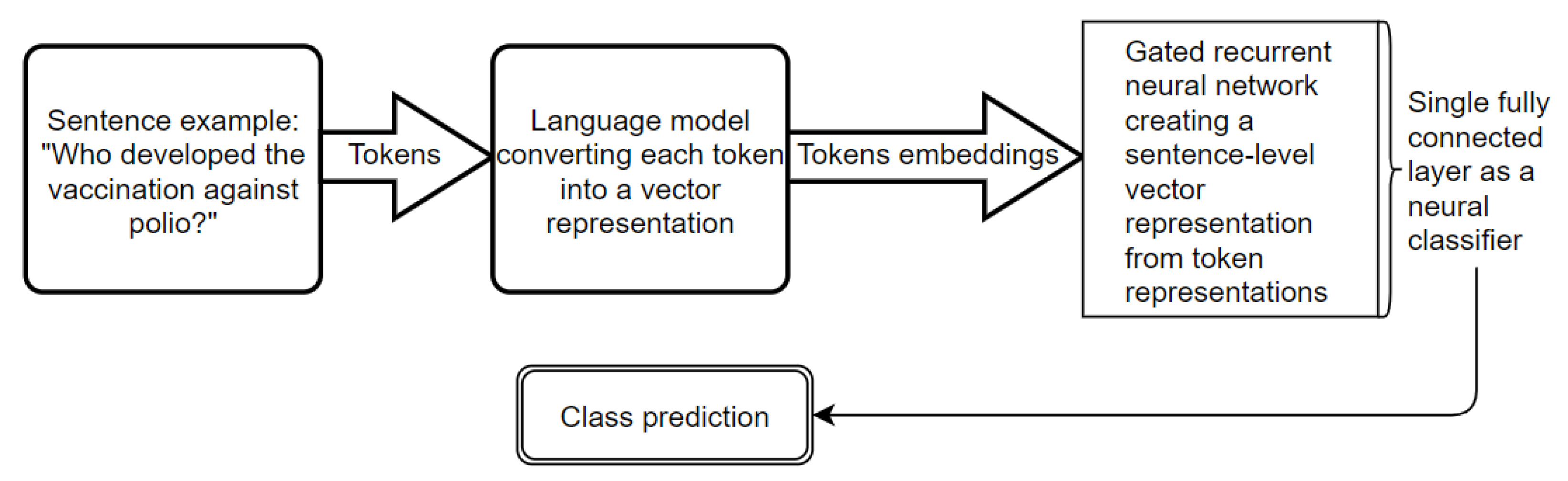
2.1. Text Classification

In this research, we used Flair v. 0.4.4 [11], an NLP framework written in PyTorch and published by the authors of the Flair LM [20]; this program enables the creation of text classification models based on various state-of-the-art LMs. With this framework, we instantiated sentence-level classifiers by using a unidirectional RNN with gated recurrent units (GRU RNN) with a single fully connected layer for final sentence classification. The GRU RNN task was to create a constant-length, sentence-level vector representation from token level embeddings provided by the selected LMs. An overall scheme presenting this workflow is presented in Figure 1. In the Flair framework, if we chose an LM enabling fine-tuning on the downstream task, e.g., BERT, the process of training the GRU RNN along with the classification layer automatically included fine-tuning of the LM.

2.2. Selection of the LMs

The LMs selected for testing are presented in

Table 1. Language models (LMs) selected for benchmarking.

LM	Publication	Comment
Glove	[1]	Static 100-dimension word embeddings, vocabulary size 400 k
Fast Text (wiki-news)	[2]	Static 300-dimension word embeddings, sub-word information, 1 M vocabulary size
Byte Pair Embeddings	[22]	Static 50-dimension sub-word embeddings, lightweight model, 100 k vocabulary size
Flair News	[20]	Combination of forward- and backward-trained models, each creating 2048-dimension word embeddings; context-aware models trained on a 1-billion-word benchmark [24]
Flair News Fast	[20]	1024-dimension version of Flair embeddings
Elmo Original	[7]	Contextualized 3072-dimension word embeddings, “original” version, 93.6 M parameters
BERT uncased large, layers −1, −2, −3, −4	[8]	Contextualized 4096-dimension embeddings, 340 M parameters, default output layers
BERT uncased large, layers 0–24, scalar mix	[8]	Contextualized 4096-dimension embeddings, 340 M parameters, scalar mix of all output layers
RoBERTa base layer −1	[23]	Contextualized 768-dimension word embeddings, base version, default output layer, 125 M parameters
RoBERTa large layer −1	[23]	Contextualized 1024-dimension word embeddings, large version, default output layer, 355 M parameters
RoBERTa large, layers 0–24, scalar Mix	[23]	Contextualized 1024-dimension word embeddings, large version with scalar mix of all output layers, 355 M parameters
XLNet layer 1	[9]	Contextualized 2048-dimension word embeddings, large-case version, default output layer, 340 M parameters
XLNey layers 0–24, scalar Mix	[9]	Contextualized 2048-dimension word embeddings, large-case version, scalar mix of all output layers, 340 M parameters
DistilBert	[25]	Contextualized 768-dimension word embeddings, 66 M parameters; model obtained through a knowledge distillation concept introduced by Hinton et al. [26]

. We chose classic LMs that provide static word-level embeddings, including Glove [1], FastText [21], a size optimized LM called BPEmb [22] that operates on a sub-word level, and a variety of recently developed deep learning LMs that create high-quality contextualized embeddings.

The complex architecture of recent models, such as BERT, Robustly Optimized BERT Pretraining Approach (RoBERTa), and XLNet, allows for choosing from many layers (heads) of the LM model that output usable token embeddings. The quality of these embeddings varies across the LM layers and even across language tasks [23]. For these LMs, we compared embeddings from the default output layer and mixing embeddings from all available output layers, as proposed in a technique called scalar mix [23].

2.3. Data Used for Benchmarking

To benchmark the selected LMs, we decided to address two-sentence classification tasks. The first was defined as the TREC6 set, a data set consisting of 5452 training questions and 500 test questions divided into six classes. The task was to classify questions as being about abbreviation, entity, description or abstract concept, human being, location, or numeric values. The class definitions in the TREC6 set were not overlapping and generally constituted a relatively easy classification task. The second task was defined by the MPD, consisting of 1000 artificial sentences that appeared as if they could have been written by an anonymous attendee of a meeting and could have come from several-sentence comments posted after that meeting. The task was to classify whether the sentence was about the following: time and punctuality, performance assessment, subject of the meeting, recommendations, or technical issues. Because the definitions of the classes were somewhat overlapping, the data set was created by three researchers who wrote and labeled the sentences independently, and because each sentence was considered outside of a wider context, this classification task was considered difficult. Notably, both benchmarked data sets had imbalanced classes (distributions presented in

Table 2. Class distributions in the analyzed data sets.

The Sixth Text REtrieval Conference (TREC6)
Class	Description	Entity	Abbreviation	Human	Location	Numerical	Total
Sentences (count)	1162	1250	86	1223	835	896	5452
Sentences (percent)	21.31	22.93	1.58	22.43	15.32	16.43	100
Meetings Preliminary Data Set (MPD)
Class	Performance Assessment	Subject	Recommendations	Time	Technical		Total
Sentences (count)	358	228	217	94	103		1000
Sentences (percent)	35.8	22.8	21.7	9.4	10.3		100

).

2.4. Performance Metrics

For drawing conclusions and discussing the statistically significant differences, the benchmark relied on the Matthews correlation coefficient (MCC) introduced by Matthews [27] because it is known to be more informative than the F1 score (F1) and class-balanced accuracy (BA) [28]. However, because F1 and CBA are widely used, we also computed them and included them in the full results published along with the MPD [18]. To address the speed of training and inference of the sentence classification framework, we report the time (hours) taken for framework training (TT) per model and time (seconds) taken to classify the entire test set (IT).

3. Methods and Procedures

3.1. Training and Testing Procedure

All computations were carried out on a single NVIDIA Titan RTX 24 GB RAM GPU. We carried out ten test runs on data splits created according to the MCCV method [29] to counter the high variance in results due to the small sizes of the data sets. The TREC6 training data were split into 80 percent training and 20 percent validation data, and tests were carried out on a set of 500 sentences officially labeled as a test. With the MPD, the procedure involved randomly choosing 100 sentences for the testing of all LMs, and according to MCCV, splitting the remaining 900 sentences ten times into 80 percent training and 20 percent validation data.

3.2. Statistics

In this paper, the results are based on statistically significant differences in the assessed parameters. Our procedure for statistical analysis began with Shapiro–Wilk [30] testing for the normality of the distribution, which led us to the conclusion that in most cases, the two distributions were normal. In the second step, we carried out one-way ANOVA. If the ANOVA indicated statistically significant differences, we carried out a third step involving Tukey HSD multiple comparison tests to assess the trials that had significant differences between them. For a test case in which the values of only one pair of parameters were compared, a Wilcoxon signed-rank test was used instead of a Tukey HSD test. The statistical analysis was carried out in Python3 (Statsmodels version ==0.10.1 and Pingouin version==0.2.9 packages). Throughout the analysis, we used a significance threshold of p = 0.05. The full results of the statistical analysis were published, along with the MPD [18].

3.3. Preliminary Study to Identify Framework Parameters and the Training Regimen

For a given LM, it is possible to select from a range of training parameter values that will affect both the training time (TT) and final model performance. Generally, training a model for a small number of epochs will provide an advantage in training time (TT) but can cause under-fitting, i.e., a negative influence on performance. If a model is trained for more epochs, TT will increase and the final model performance can increase, but it is not guaranteed due to a negative over-fitting phenomenon.

Therefore, before benchmarking the effects of the chosen LMs on the quality and speed of the training and the sentence classification, we carried out a preliminary study to determine the impact of the hyperparameters and the training parameters of the framework on our classification tasks.

Our work examined various parameters from a group of learning-rate-related parameters: (a) Learning rate—the step size at each iteration while moving toward a minimum of a loss function [31]; we tested values of 0.3, 0.2, 0.15, 0.1, and 0.05. (b) Initial learning rate—the learning rate that the model is trained with during the first epoch. (c) Patience—the number of epochs the model is trained with a given learning rate after the last improvement of model performance in a given step and before annealing of the learning rate. For example, given patience equal to 10, if the performance improved during training at the current learning rate only in the 3rd epoch, even without improvement in performance in any other epoch of the executed step, the training will proceed up to 3 + 10 epochs at the given learning rate. In our experiments, values of 5, 10, 15, 20, and 25 were tested. (d) Annealing factor—the ratio of decreasing the learning rate. Annealing factor × previous learning rate = current learning rate. In our experiments values of 0.3, 0.4, and 0.5 were considered. (e) Minimal learning rate—a minimal threshold learning rate. When computing the learning rate for the next training step according to the equation: learning rate × anneal factor results in a value lower than minimal learning rate, the model training is terminated. Our work experimented with values of 0.01, 0.008, 0.002, 0.001, and 0.0001.

Other considered parameters affecting the speed and quality of the model performance included: (1) The size of a mini-batch, i.e., the number of data instances provided at the same time on a model input during training, where values of 4, 8, 32, and 64 were considered. (2) The RNN hidden size, which defines the size of the vector representation of a sentence created by the RNN from token level embeddings, where values of 2, 16, 128, 256, and 512 were considered. (3) Shuffling sentences provided to the framework during training (true or false) were analyzed. Other framework parameters were set to default, as proposed by the authors of the Flair framework.

All trials during the preliminary study were computed with the FastText (“en-news”) LM [2] with 1 million static word vectors. The initial study was carried out on both the TREC6 set and the MPD to demonstrate possible differences that could be attributed to the data set selection. Preliminary results from the TREC6 data set were considered decisive regarding the selection of training parameters for the final experiment as this data set consisted of over five times more data instances. When assessing the results of our preliminary study regarding training-related parameters, we considered only the MCC scores and TT of the framework. However, because the hidden size can also affect the IT, in this case, we also included it in the results.

Because the purpose of the study was to compare various LMs in the same training conditions, which most likely do not provide the highest possible performance for all LMs, for the final experiment, we selected training parameters that probably caused the models to be slightly under-fitted but provided a rather low TT. If one aimed for a training procedure that guarantees the top performance, a much longer TT must be considered and the training regime should be fitted precisely to both the LM and the data set.

3.4. Principal Component Analysis for Visualization of the LMs’ Quality

To visualize discrepancies between the baseline and state-of-the-art LMs, we carried out a two-component principal component analysis of sentence embeddings provided by the framework using GloVe and RoBERTa large scalar mix LMs. The sentence-level vector representations were computed for all 1000 sentences from the MPD. Each sentence embedding was accompanied by an original class label, which allowed us to inspect the quality of grouping each class using the analyzed LM.

4. Results and Discussion

4.1. Preliminary Study

Figure 2 shows that increasing the size of the sentence-level vector representation created by the RNN increased the TT. Simultaneously, for the short questions in the TREC6 data set, sentence embeddings as short as 16 elements enabled high performance. A higher dimensionality of sentence embeddings did not appear to improve the MCC score since no statistically significant differences were found; however, owing to a relatively low increase in the TT, we used a hidden size of 256 to ensure that we provided sufficient space for the information present in the sentences.

Figure 3 illustrates the effect of the mini-batch size on the framework performance, given a time-consuming training regimen. For the given setup, there were no statistically significant differences in the MCC scores with small mini-batch sizes of 4 and 8. However, the small mini-batch sizes were significantly superior to the higher values of 32 and 64. Additionally, the TT with a mini-batch size of 8 was significantly shorter than that with a batch size of 4. Therefore, we used a mini-batch size of 8. The full results of the statistical analysis have been published, along with the MPD and python code used in our research [18].

Figure 4 presents the effect of shuffling examples during training. With shuffling, the framework achieved higher MCC values, and the differences were statistically significant. Therefore, we decided to shuffle the training examples.

Table 3. Impact of the learning-rate-related parameters on the framework performance for the TREC6 set and the MPD given a mini-batch size = 8, hidden size = 256, shuffle = True. Compared variants were named with use of abbreviations: p—patience, lr—initial learning rate, mlr—minimal learning rate, a—annealing. For example, p5lr.1mlr.0001a.5 stands for patience = 5, initial learning rate = 0.1, minimal learning rate = 0.0001, and annealing factor = 0.5. The final training regime selected for the final LM comparison is highlighted in bold.

	MCC Score		Training Time (TT)
Training Regime	MPD	TREC6	MPD	TREC6
p5lr.1mlr.0001a.5	0.475 ± 0.042	0.923 ± 0.007	0.051 ± 0.008	0.362 ± 0.037
p10lr.1mlr.0001a.5	0.477 ± 0.054	0.923 ± 0.01	0.079 ± 0.018	0.56 ± 0.087
p15lr.1mlr.0001a.5	0.477 ± 0.044	0.925 ± 0.007	0.103 ± 0.011	0.699 ± 0.094
p20lr.1mlr.0001a.5	0.472 ± 0.029	0.928 ± 0.005	0.145 ± 0.026	0.761 ± 0.057
p25lr.1mlr.0001a.5	0.468 ± 0.03	0.931 ± 0.008	0.158 ± 0.029	0.91 ± 0.067
p20lr.1mlr.001a.4	0.473 ± 0.043	0.928 ± 0.008	0.1 ± 0.02	0.438 ± 0.057
p20lr.2mlr.01a.5	0.475 ± 0.056	0.92 ± 0.015	0.082 ± 0.02	0.367 ± 0.078
p5lr.2mlr.008a.5	0.437 ± 0.05	0.92 ± 0.015	0.042 ± 0.01	0.167 ± 0.031
p10lr.05mlr.001a.5	0.477 ± 0.055	0.916 ± 0.012	0.063 ± 0.011	0.359 ± 0.042
p15lr.1mlr.001a.5	0.471 ± 0.049	0.929 ± 0.005	0.086 ± 0.01	0.618 ± 0.096
p10lr.3mlr.01a.3	0.484 ± 0.027	0.898 ± 0.012	0.051 ± 0.013	0.119 ± 0.02
p25lr.15mlr.001a.5	0.463 ± 0.04	0.934 ± 0.007	0.132 ± 0.025	0.645 ± 0.112
p20lr.1mlr.002a.5	0.487 ± 0.046	0.933 ± 0.005	0.098 ± 0.014	0.269 ± 0.02

depicts the influence of the training-rate-related parameters on the performance and TT of the adopted framework for the TREC6 set and the MPD. The performance discrepancies for the MPD and the TREC6 set measured in points of the mean MCC score were 0.05 and 0.036, respectively. When the mean TT was considered, the differences were up to 0.116 h for the MPD and 0.643 h for the TREC6 set. It can be observed that the relation of the TT achieved in various test runs was very similar in both data sets. This allowed us to hypothesize that the relation of the TT between test runs did not vary strongly with the choice of data set. However, this was not the case when the LMs quality was concerned. We believe that the proposed training regimes for the TREC6 data set, when applied to the MPD, caused each model to be as well trained, with only one exception of a very short training scheme p5lr.2mlr.008a.5. This was likely caused by the smaller size of the MPD, which allowed the LMs to fit the data in a shorter time.

Based on this exploratory study, we decided to use a training regimen providing almost the best performance for both the TREC6 set and the MPD, namely p20lr.1mlr.002a.5. For the TREC6 set, the selected training procedure allowed for a 0.933 mean MCC score at a decent TT cost of a median of 0.269 h per trained model. Therefore, the configuration of the adopted framework in the final LM comparison was as follows: patience = 20, initial learning rate = 0.1, minimal learning rate = 0.002, annealing factor = 0.5, mini-batch size = 8, hidden size = 256, with example shuffling during training.

4.2. Results of the Main Study

A comparison of selected LMs in the previously described framework was carried out on two data sets. The results obtained with the TREC6 data set are presented in Figure 5. The results obtained with the preliminary data set are shown in Figure 6.

The results presented in Figure 5 indicated that the baseline provided by static embeddings created by Glove and FastText was high and reached a 0.933 ± 0.005 MCC score. Recent transformer-based models outperformed this baseline and have achieved up to a 0.96 ± 0.006 MCC score for the BERT large uncased scalar mix version. Simultaneously, the MCC scores achieved by RoBERTa, XLNet, and variants of these models were unexpectedly worse than those of BERT for several possible reasons, such as incorrect training regimens for these LMs and data set properties. Generally, these results may indicate that, given the small differences in quality and the small data set size, to distinguish among very good models, a similar benchmark analysis must be used on an n-times-larger data set.

Simultaneously, the results achieved on the MPD (see Figure 6) revealed a different picture. A large and statistically significant discrepancy was observed between the MCC scores of the baseline LMs providing static word embeddings, such as Glove (0.402 ± 0.051) or FastText (0.47 ± 0.047), and state-of-the-art context-aware LMs, such as RoBERTa (0.59 ± 0.026). Leveraging the scalar mix technique allowed us to use the output from all available layers of these complex models and thus achieve the best results in all tested model pairs. The default layer of the XLNet achieved a very poor result of 0.377 ± 0.063, whereas the scalar mix version achieved 0.521 ± 0.038; the straightforward BERT scored 0.532 ± 0.043 and its scalar mix counterpart scored 0.596 ± 0.027; and the RoBERTa and RoBERTa scalar mix version achieved 0.59 ± 0.026 and 0.603 ± 0.023, respectively. Therefore, the scalar mix technique appeared to be highly useful, in agreement with findings from Liu et al. [32]. However, the increase in quality came at the expense of both TT and IT. As expected, the IT was the lowest for LMs providing static embeddings, reaching as low as 0.111 ± 0.011 s per 100 sentences for the FastText LM. The highest inference time of 3.822 ± 0.015 was obtained with the XLNet scalar mix LM. Additionally, the TTs of the contextualized LMs in their scalar mix versions were the highest, reaching 1.444 ± 0.175 h for the XLNet scalar mix LM, whereas the baseline Glove-based framework required only 0.069 ± 0.011 h to train.

The results for the MPD allowed us to visualize different qualities of various LMs grouping sentences by classes. Figure 7 presents a visualization based on a principal component analysis, which indicates that the Glove-based framework was unable to clearly divide classes, whereas the RoBERTa large scalar mix LM was able to distinguish groups with significantly higher quality.

5. Conclusions

A comparison of the results obtained for the TREC6 set and the MPD suggested that they differed strongly in the magnitude of the MCC scores. For the TREC6 set, almost all LMs achieved MCC scores greater than 0.9, whereas on the MPD, the highest values were only slightly above 0.6, and the lowest values were below 0.4. The finding that even LMs creating static embeddings achieved very good results on the TREC6 data set was due to the simplicity of the classification tasks. Consequently, there was little room for improvement of state-of-the-art LMs, thus making any conclusions regarding the quality of newer LMs difficult to draw. In contrast, the MPD was challenging because using simple static word embeddings allowed for a 0.47 ± 0.047 MCC score at best. However, interestingly, the sophisticated context-aware LMs demonstrated their superiority on the MPD since they were able to locate the necessary information in sentences full of contextual meaning and achieve scores of up to 0.603 ± 0.023. From these results, we postulate that for context-aware LMs to fully demonstrate their advantages, a sufficiently difficult task must be used.

A similar phenomenon was encountered in a deep learning task from another domain, namely the detection of objects in image analysis. Owing to the progress in the quality of solutions offered by models using complex convolutional neural network architectures, the differences in performance on once broadly addressed Pascal Voc data set became very small. Many models were able to achieve up to an 80 percent mean average precision score [33]. A solution was proposed by the MS CoCo challenge [34], in which the metrics emphasized the need for more precise localization of detected objects, thus increasing the task difficulty. As a result, the state-of-the-art models achieved a less than 50 percent mean average precision score in this challenge [35], thus leaving a lot of room for further improvement and demonstration of high-quality solutions. Unfortunately, owing to the very small size of the MPD, other explanations for this phenomenon cannot be excluded: some newer deep learning models might enable the framework to learn properly even given the small amount of data, or a framework based on baseline LMs might simply need more data. To rule out these possibilities, a larger yet still challenging data set would be required.

6. Study Limitations and Future Work

The presented comparison was carried out on two small data sets, thus resulting in a high standard deviation of the results. In assessing differences between models achieving similar median MCC scores, i.e., differing by less than 0.01 point on the TREC6 set, before drawing any conclusions, the standard deviation exceeding 0.01 points in some cases must be considered. The TREC6 data set appeared to be insufficiently difficult for examining differences in state-of-the-art LMs. Therefore, our future work will aim at increasing the MPD size to rule out all the negative effects of the small analyzed data sample and to allow us to draw stronger conclusions on a more challenging data set. Another limitation of the study was associated with our preliminary study, in which we decided to select one set of hyperparameters and training parameters for all selected LMs. Such a decision provided a common ground for the whole comparison. However, it also had a negative impact, namely the selected training regime was most likely favorable for some of the LMs and we have no information about which ones. A contradictory approach could be to search for training parameters separately for each selected LM. Pursuing this line of the experiment would lead to a situation where probably almost all LMs should have their original training regimes and one would end up comparing “training-optimized” versions of each LM. Such an approach would also have its imperfections; for example, it can be very time-consuming for state-of-the-art LMs, and in the end, would put the researcher in a situation of comparing LMs trained with entirely different procedures.

References

1. Pennington, J.; Socher, R.; Manning, C. Glove: Global vectors for word representation. In Proceedings of the 2014 Conference on Empirical Methods in Natural Language Processing (EMNLP), Doha, Qatar, 25–29 October 2014; pp. 1532–1543. [Google Scholar]
2. Mikolov, T.; Chen, K.; Corrado, G.; Dean, J. Efficient estimation of word representations in vector space. arXiv 2013, arXiv:1301.3781. [Google Scholar]
3. Vosoughi, S.; Vijayaraghavan, P.; Roy, D. Tweet2vec: Learning tweet embeddings using character-level cnn-lstm encoder-decoder. In Proceedings of the 39th International ACM SIGIR Conference on Research and Development in Information Retrieval, Pisa, Italy, 17–21 July 2016; pp. 1041–1044. [Google Scholar]
4. Santos, C.D.; Zadrozny, B. Learning character-level representations for part-of-speech tagging. In Proceedings of the 31st International Conference on Machine Learning (ICML-14), Bejing, China, 22–24 June 2014; pp. 1818–1826. [Google Scholar]
5. Santos, C.N.D.; Guimaraes, V. Boosting named entity recognition with neural character embeddings. arXiv 2015, arXiv:1505.05008. [Google Scholar]
6. Prabhu, A.; Joshi, A.; Shrivastava, M.; Varma, V. Towards sub-word level compositions for sentiment analysis of hindi-english code mixed text. arXiv 2016, arXiv:1611.00472. [Google Scholar]
7. Peters, M.E.; Neumann, M.; Iyyer, M.; Gardner, M.; Clark, C.; Lee, K.; Zettlemoyer, L. Deep contextualized word representations. arXiv 2018, arXiv:1802.05365. [Google Scholar]
8. Devlin, J.; Chang, M.W.; Lee, K.; Toutanova, K. BERT: Pre-training of deep bidirectional transformers for language understanding. arXiv 2018, arXiv:1810.04805. [Google Scholar]
9. Yang, Z.; Dai, Z.; Yang, Y.; Carbonell, J.; Salakhutdinov, R.; Le, Q.V. XLNet: Generalized Autoregressive Pretraining for Language Understanding. arXiv 2019, arXiv:1906.08237. [Google Scholar]
10. Beloki, Z.; Artola, X.; Soroa, A. A scalable architecture for data-intensive natural language processing. Nat. Lang. Eng. 2017, 23, 709–731. [Google Scholar] [CrossRef]
11. Akbik, A.; Bergmann, T.; Blythe, D.; Rasul, K.; Schweter, S.; Vollgraf, R. Flair: An easy-to-use framework for state-of-the-art nlp. In Proceedings of the 2019 Conference of the North American Chapter of the Association for Computational Linguistics (Demonstrations), Minneapolis, MN, USA, 2–7 June 2019; pp. 54–59. [Google Scholar]
12. Gardner, M.; Grus, J.; Neumann, M.; Tafjord, O.; Dasigi, P.; Liu, N.; Zettlemoyer, L. Allennlp: A deep semantic natural language processing platform. arXiv 2018, arXiv:1803.07640. [Google Scholar]
13. Cer, D.; Yang, Y.; Kong, S.Y.; Hua, N.; Limtiaco, N.; John, R.S.; Constant, N.; Guajardo-Cespedes, M.; Yuan, S.; Tar, C.; et al. Universal sentence encoder. arXiv 2018, arXiv:1803.11175. [Google Scholar]
14. Perone, C.S.; Silveira, R.; Paula, T.S. Evaluation of sentence embeddings in downstream and linguistic probing tasks. arXiv 2018, arXiv:1806.06259. [Google Scholar]
15. Conneau, A.; Kiela, D.; Schwenk, H.; Barrault, L.; Bordes, A. Supervised learning of universal sentence representations from natural language inference data. arXiv 2017, arXiv:1705.02364. [Google Scholar]
16. Talman, A.; Yli-Jyrä, A.; Tiedemann, J. Sentence Embeddings in NLI with Iterative Refinement Encoders. arXiv 2018, arXiv:1808.08762. [Google Scholar] [CrossRef] [Green Version]
17. Li, X.; Roth, D. Learning question classifiers. In Proceedings of the 19th international Conference on Computational linguistics-Volume 1, Taipei, Taiwan,, 24 August–1 September 2002; Association for Computational Linguistics: Stroudsburg, PA, USA, 2002; pp. 1–7. [Google Scholar]
18. Fiok, K. Meetings Preliminary Data Set. 2019. Available online: https://github.com/krzysztoffiok/MPD-data set (accessed on 15 January 2020).
19. Xu, Q.S.; Liang, Y.Z. Monte Carlo cross validation. Chemometr. Intell. Lab. Syst. 2001, 56, 1–11. [Google Scholar] [CrossRef]
20. Akbik, A.; Blythe, D.; Vollgraf, R. Contextual string embeddings for sequence labeling. In Proceedings of the 27th International Conference on Computational Linguistics, Santa Fe, NM, USA, 20–26 August 2018; pp. 1638–1649. [Google Scholar]
21. Mikolov, T.; Grave, E.; Bojanowski, P.; Puhrsch, C.; Joulin, A. Advances in pre-training distributed word representations. arXiv 2017, arXiv:1712.09405. [Google Scholar]
22. Heinzerling, B.; Strube, M. Bpemb: Tokenization-free pre-trained subword embeddings in 275 languages. arXiv 2017, arXiv:1710.02187. [Google Scholar]
23. Liu, Y.; Ott, M.; Goyal, N.; Du, J.; Joshi, M.; Chen, D.; Levy, O.; Lewis, M.; Zettlemoyer, L.; Stoyanov, V. RoBERTa: A robustly optimized BERT pretraining approach. arXiv 2019, arXiv:1907.11692. [Google Scholar]
24. Chelba, C.; Mikolov, T.; Schuster, M.; Ge, Q.; Brants, T.; Koehn, P.; Robinson, T. One billion word benchmark for measuring progress in statistical language modeling. arXiv 2013, arXiv:1312.3005. [Google Scholar]
25. Sanh, V.; Debut, L.; Chaumond, J.; Wolf, T. DistilBERT, a distilled version of BERT: Smaller, faster, cheaper and lighter. arXiv 2019, arXiv:1910.01108. [Google Scholar]
26. Hinton, G.; Vinyals, O.; Dean, J. Distilling the knowledge in a neural network. arXiv 2015, arXiv:1503.02531. [Google Scholar]
27. Matthews, B.W. Comparison of the predicted and observed secondary structure of T4 phage lysozyme. Biochim. Biophys. Acta (BBA)-Protein Struct. 1975, 405, 442–451. [Google Scholar] [CrossRef]
28. Chicco, D. Ten quick tips for machine learning in computational biology. BioData Min. 2017, 10, 35. [Google Scholar] [CrossRef]
29. Dubitzky, W.; Granzow, M.; Berrar, D.P. (Eds.) Fundamentals of Data Mining in Genomics and Proteomics; Springer Science & Business Media: New York, NY, USA, 2007. [Google Scholar]
30. Shapiro, S.S.; Wilk, M.B. An analysis of variance test for normality (complete samples). Biometrika 1965, 52, 591–611. [Google Scholar] [CrossRef]
31. Murphy, K.P. Machine Learning: A Probabilistic Perspective; MIT Press: Cambridge, MA, USA, 2012; p. 247. ISBN 978-0-262-01802-9. [Google Scholar]
32. Liu, N.F.; Gardner, M.; Belinkov, Y.; Peters, M.; Smith, N.A. Linguistic knowledge and transferability of contextual representations. arXiv 2019, arXiv:1903.08855. [Google Scholar]
33. Shen, Z.; Liu, Z.; Li, J.; Jiang, Y.G.; Chen, Y.; Xue, X. Object detection from scratch with deep supervision. IEEE Trans. Pattern Anal. Mach. Intell. 2019, 42, 398–412. [Google Scholar] [CrossRef] [Green Version]
34. Lin, T.Y.; Maire, M.; Belongie, S.; Hays, J.; Perona, P.; Ramanan, D.; Dollár, P.; Zitnick, C.L. Microsoft coco: Common objects in context. In Proceedings of the European Conference on Computer Vision, Zurich, Switzerland, 6–12 September 2014; Springer: Cham, Switzerland, 2014; pp. 740–755. [Google Scholar]
35. Li, Y.; Chen, Y.; Wang, N.; Zhang, Z. Scale-aware trident networks for object detection. arXiv 2019, arXiv:1901.01892. [Google Scholar]
Figure 1. Sentence classification workflow in the adopted framework.
Applsci 10 03386 g001
Figure 2. Impact of the hidden size on the framework performance given a time-consuming training regimen (initial learning rate = 0.1, minimal learning rate = 0.0001, annealing factor = 0.5, patience = 20, mini-batch size = 32, shuffle = True) on the TREC6 data set. MCC: Matthews Correlation Coefficient.
Applsci 10 03386 g002
Figure 3. Impact of the mini-batch size on the framework performance given a time-consuming training regimen (initial learning rate = 0.1, minimal learning rate = 0.0001, annealing factor = 0.5, patience = 20, hidden size = 256, shuffle = True) on the TREC6 data set.
Applsci 10 03386 g003
Figure 4. Effect of shuffling the training examples on the framework performance given a time-consuming training regimen (initial learning rate = 0.1, minimal learning rate = 0.0001, annealing factor = 0.5, patience = 20, hidden size = 256, batch size = 32) on the TREC6 data set.
Applsci 10 03386 g004
Figure 5. Comparison of framework performance with selected language models on the TREC6 data set. Explanation of the abbreviated names of LMs: S—scalar mix, L—large model version. Example notation RoBERTa LS stands for RoBERTa large scalar mix model.
Applsci 10 03386 g005
Figure 6. Comparison of framework performance with selected language models on the MPD. Explanation of the abbreviated names of LMs: S—scalar mix, L—large model version. Example notation RoBERTa LS stands for RoBERTa large scalar mix model.
Applsci 10 03386 g006
Figure 7. Visual comparison of the baseline and state-of-the-art LMs. Principle component analysis (PCA) of sentence embeddings computed for the whole MPD by frameworks based on GloVe (left) and RoBERTa large scalar mix (right) LMs. Class labels are represented by colors: red—performance assessment, green—subject, blue—recommendations, black—technical, and magenta—time.
Applsci 10 03386 g007