Two-Dimensional Histogram Shifting-Based Reversible Data Hiding for H.264/AVC Video


Abstract
1. Introduction
2. HS-based RDH Technique
3. Proposed Schemes
3.1. Analysis of 2D HS-based RDH Schemes in Compressed Domain
3.1.1. Related Schemes Using the Coefficient Pairs
3.1.2. Related Schemes Without Using the Coefficient Pairs
3.2. Proposed 2D HS-Based RDH Schemes
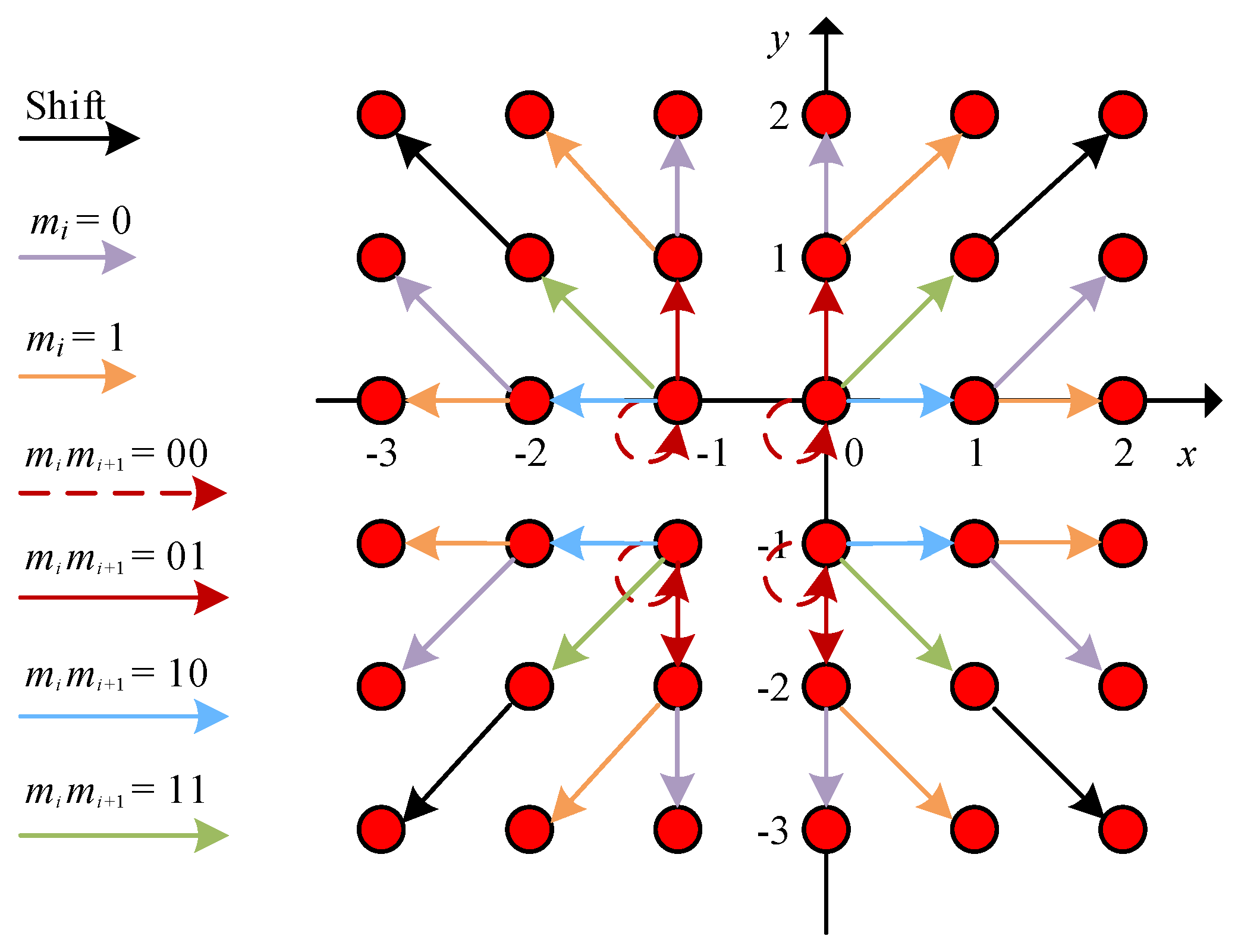
3.2.1. 2D HS Using the Coefficient Pairs
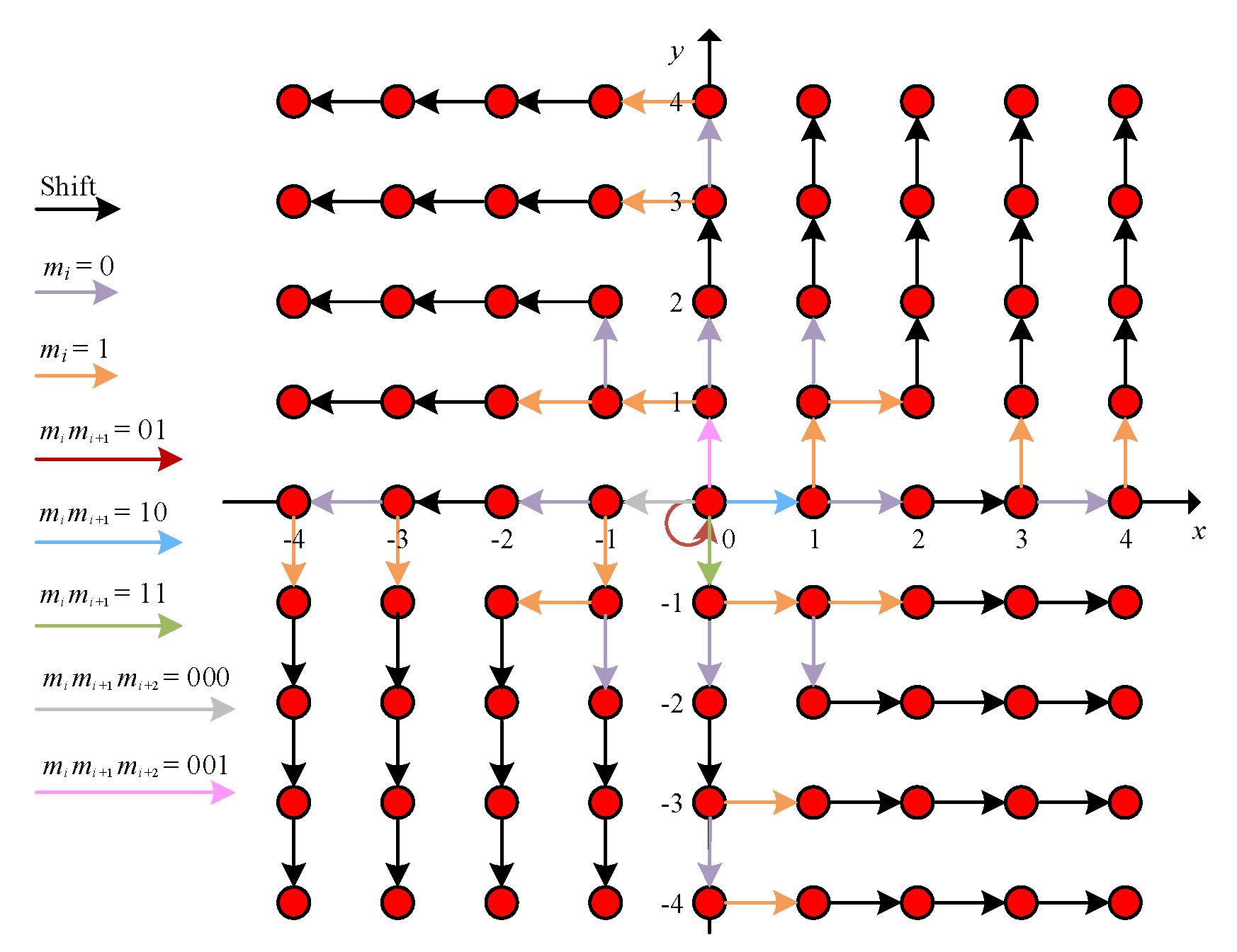
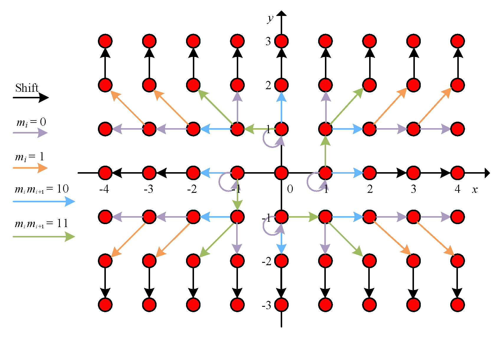
3.2.2. 2D HS without Using the Coefficient Pairs
3.2.3. Data Extraction and Video Recovery
4. Experimental Results
4.1. Embedding Capacity
4.2. Video Quality
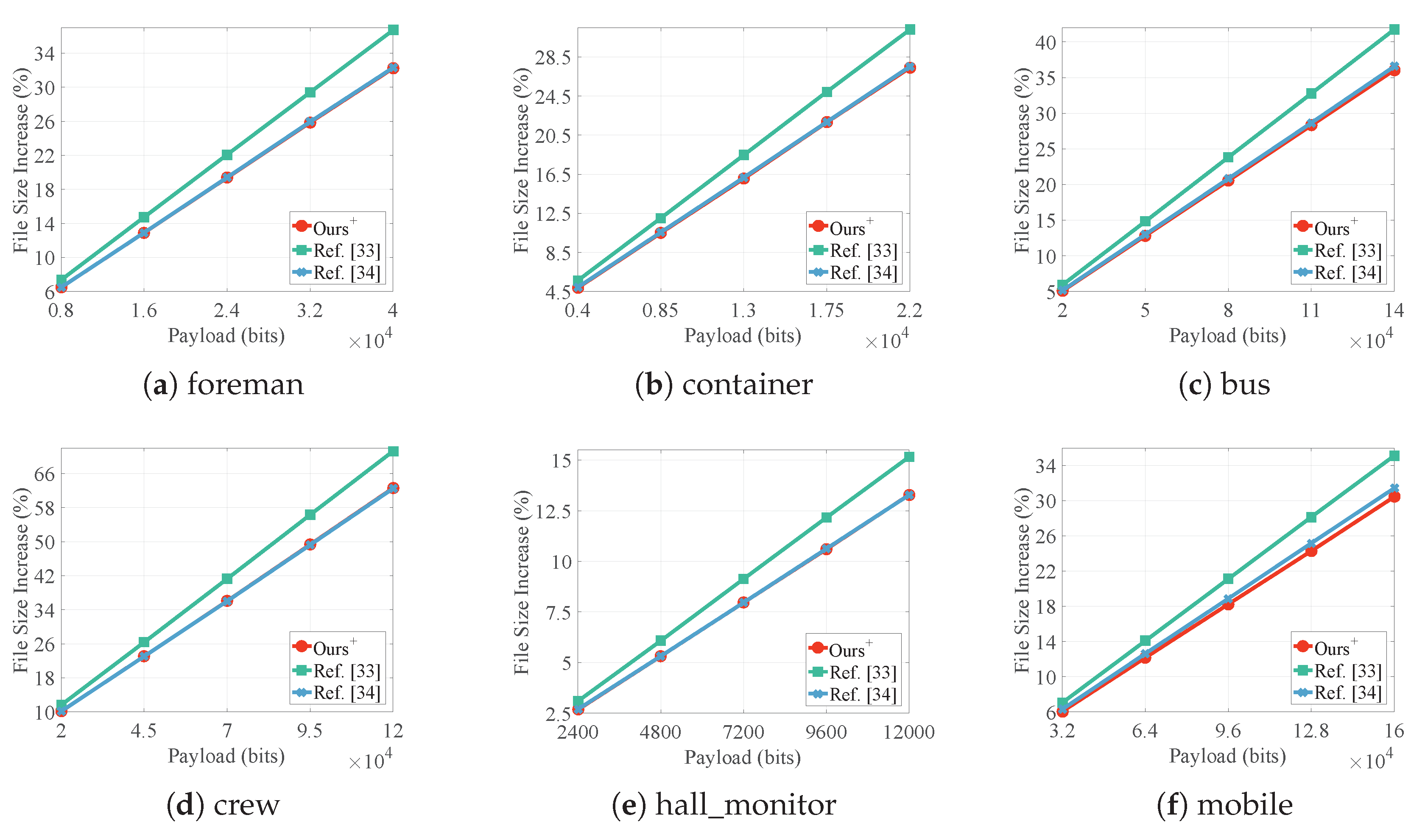
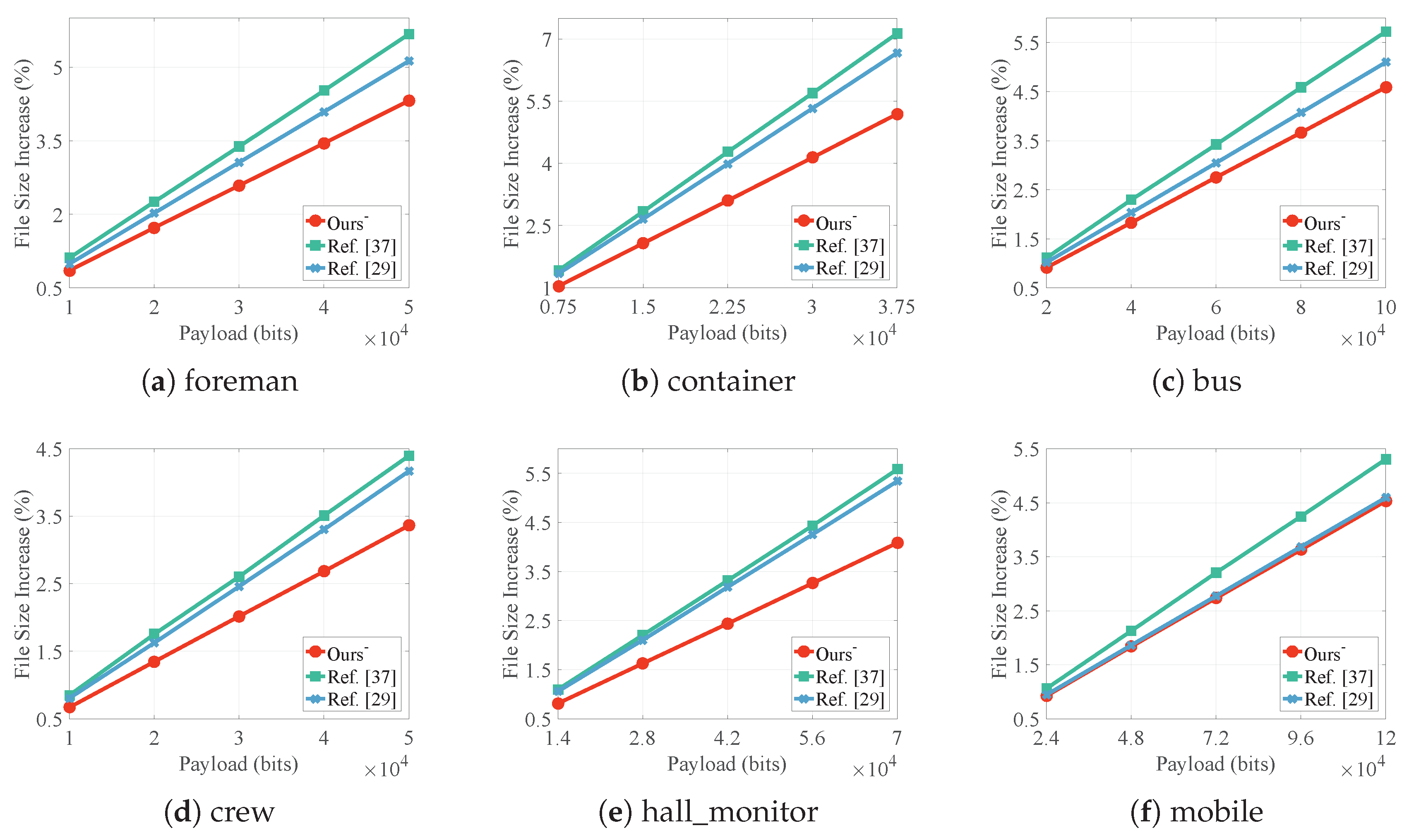
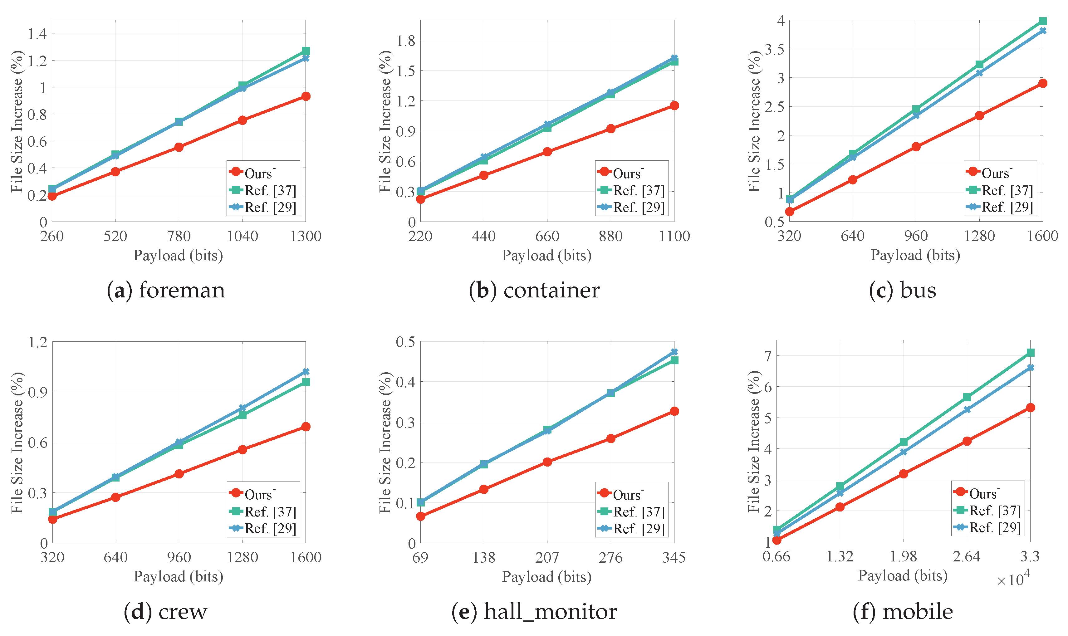
4.3. File Size
5. Conclusions
Author Contributions
Funding
Conflicts of Interest
References
- Goljan, M.; Fridrich, J.J.; Du, R. Distortion-Free Data Embedding for Images. In Proceedings of the Information Hiding (IH’01), Pittsburgh, PA, USA, 25–27 April 2001; Volume 2137, pp. 27–41. [Google Scholar]
- Celik, M.U.; Sharma, G.; Tekalp, A.M.; Saber, E. Lossless Generalized-LSB Data Embedding. IEEE Trans. Image Process. 2005, 14, 253–266. [Google Scholar] [CrossRef] [PubMed]
- Tian, J. Reversible Data Embedding Using a Difference Expansion. IEEE Trans. Circuits Syst. Video Technol. 2003, 13, 890–896. [Google Scholar] [CrossRef]
- Hu, Y.; Lee, H.K.; Chen, K.; Li, J. Difference Expansion Based Reversible Data Hiding Using Two Embedding Directions. IEEE Trans. Multimed. 2008, 10, 1500–1512. [Google Scholar] [CrossRef]
- Liu, M.; Seah, H.S.; Zhu, C.; Lin, W.; Tian, F. Reducing Location Map in Prediction-based Difference Expansion for Reversible Image Data Embedding. Signal Process. 2012, 92, 819–828. [Google Scholar] [CrossRef]
- Caciula, I.; Coanda, H.G.; Coltuc, D. Multiple Moduli Prediction Error Expansion Reversible Data Hiding. Signal Process. Image Commun. 2019, 71, 120–127. [Google Scholar] [CrossRef]
- Ni, Z.; Shi, Y.Q.; Ansari, N.; Su, W. Reversible Data Hiding. IEEE Trans. Circuits Syst. Video Technol. 2006, 16, 354–362. [Google Scholar]
- Lin, C.C.; Tai, W.L.; Chang, C.C. Multilevel Reversible Data Hiding Based on Histogram Modification of Difference Images. Pattern Recognit. 2008, 41, 3582–3591. [Google Scholar] [CrossRef]
- Tai, W.L.; Yeh, C.M.; Chang, C.C. Reversible Data Hiding Based on Histogram Modification of Pixel Differences. IEEE Trans. Circuits Syst. Video Technol. 2009, 19, 906–910. [Google Scholar]
- Hong, W.; Chen, T.S.; Shiu, C.W. Reversible Data Hiding for High Quality Images Using Modification of Prediction Errors. J. Syst. Softw. 2009, 82, 1833–1842. [Google Scholar] [CrossRef]
- Kim, S.; Qu, X.; Sachnev, V.; Kim, H.J. Skewed Histogram Shifting for Reversible Data Hiding Using a Pair of Extreme Predictions. IEEE Trans. Circuits Syst. Video Technol. 2018, 29, 3236–3246. [Google Scholar] [CrossRef]
- Jia, Y.; Yin, Z.; Zhang, X.; Luo, Y. Reversible Data Hiding Based on Reducing Invalid Shifting of Pixels in Histogram Shifting. Signal Process. 2019, 163, 238–246. [Google Scholar] [CrossRef]
- Jung, S.M.; On, B.W. An Advanced Reversible Data Hiding Algorithm Using Local Similarity, Curved Surface Characteristics, and Edge Characteristics in Images. Appl. Sci. 2020, 10, 836. [Google Scholar] [CrossRef]
- Li, X.; Zhang, W.; Gui, X.; Yang, B. Efficient Reversible Data Hiding Based on Multiple Histograms Modification. IEEE Trans. Inf. Forensics Secur. 2015, 10, 2016–2027. [Google Scholar]
- Wang, J.; Ni, J.; Zhang, X.; Shi, Y.Q. Rate and Distortion Optimization for Reversible Data Hiding Using Multiple Histogram Shifting. IEEE Trans. Cybern. 2017, 47, 315–326. [Google Scholar] [CrossRef] [PubMed]
- Ou, B.; Zhao, Y. High Capacity Reversible Data Hiding Based on Multiple Histograms Modification. IEEE Trans. Circuits Syst. Video Technol. 2019. [Google Scholar] [CrossRef]
- Wang, J.; Chen, X.; Ni, J.; Mao, N.; Shi, Y. Multiple Histograms Based Reversible Data Hiding: Framework and Realization. IEEE Trans. Circuits Syst. Video Technol. 2019. [Google Scholar] [CrossRef]
- Li, X.; Zhang, W.; Gui, X.; Yang, B. A Novel Reversible Data Hiding Scheme Based on Two-Dimensional Difference-Histogram Modification. IEEE Trans. Inf. Forensics Secur. 2013, 8, 1091–1100. [Google Scholar]
- Ou, B.; Li, X.; Zhao, Y.; Ni, R.; Shi, Y. Pairwise Prediction-Error Expansion for Efficient Reversible Data Hiding. IEEE Trans. Image Process. 2013, 22, 5010–5021. [Google Scholar] [CrossRef]
- Ou, B.; Li, X.; Zhang, W.; Zhao, Y. Improving Pairwise PEE Via Hybrid-dimensional Histogram Generation and Adaptive Mapping Selection. IEEE Trans. Circuits Syst. Video Technol. 2018, 29, 2176–2190. [Google Scholar] [CrossRef]
- Xiao, M.; Li, X.; Wang, Y.; Zhao, Y.; Ni, R. Reversible Data Hiding Based on Pairwise Embedding and Optimal Expansion Path. Signal Process. 2019, 158, 210–218. [Google Scholar] [CrossRef]
- Wu, H.; Mai, W.; Meng, S.; Cheung, Y.; Tang, S. Reversible Data Hiding With Image Contrast Enhancement Based on Two-Dimensional Histogram Modification. IEEE Access 2019, 7, 83332–83342. [Google Scholar] [CrossRef]
- Qin, J.; Huang, F. Reversible Data Hiding Based on Multiple Two-Dimensional Histograms Modification. IEEE Signal Process. Lett. 2019, 26, 843–847. [Google Scholar] [CrossRef]
- Huang, F.; Qu, X.; Kim, H.J.; Huang, J. Reversible Data Hiding in JPEG Images. IEEE Trans. Circuits Syst. Video Technol. 2016, 26, 1610–1621. [Google Scholar] [CrossRef]
- Qian, Z.; Dai, S.; Chen, B. Reversible Data Hiding in JPEG Images Using Ordered Embedding. KSII Trans. Internet Inf. Syst. 2017, 11, 945–958. [Google Scholar]
- Wedaj, F.T.; Kim, S.; Kim, H.J.; Huang, F. Improved Reversible Data Hiding in JPEG Images Based on New Coefficient Selection Strategy. EURASIP J. Image Video Process. 2017, 2017, 63. [Google Scholar] [CrossRef]
- Hou, D.; Wang, H.; Zhang, W.; Yu, N. Reversible Data Hiding in JPEG Image Based on DCT Frequency and Block Selection. Signal Process. 2018, 148, 41–47. [Google Scholar] [CrossRef]
- He, J.; Chen, J.; Tang, S. Reversible Data Hiding in JPEG Images Based on Negative Influence Models. IEEE Trans. Inf. Forensics Secur. 2020, 15, 2121–2133. [Google Scholar] [CrossRef]
- Cheng, S.; Huang, F. Reversible Data Hiding in JPEG Images Based on Two-Dimensional Histogram Modification. In Proceedings of the 4th International Conference on Cloud Computing and Security (ICCCS’18), Haikou, China, 8–10 June 2018; pp. 392–403. [Google Scholar]
- Chung, K.; Huang, Y.; Chang, P.; Liao, H.M. Reversible Data Hiding-Based Approach for Intra-Frame Error Concealment in H.264/AVC. IEEE Trans. Circuits Syst. Video Technol. 2010, 20, 1643–1647. [Google Scholar] [CrossRef]
- Fallahpour, M.; Shirmohammadi, S.; Ghanbari, M. A High Capacity Data Hiding Algorithm for H.264/AVC Video. Secur. Commun. Netw. 2015, 8, 2947–2955. [Google Scholar] [CrossRef]
- Liu, Y.; Ju, L.; Hu, M.; Ma, X.; Zhao, H. A Robust Reversible Data Hiding Scheme for H.264 without Distortion Drift. Neurocomputing 2015, 151, 1053–1062. [Google Scholar] [CrossRef]
- Xu, D.; Wang, R. Two-dimensional Reversible Data Hiding-based Approach for Intra-Frame Error Concealment in H.264/AVC. Signal Process. Image Commun. 2016, 47, 369–379. [Google Scholar] [CrossRef]
- Zhao, J.; Li, Z.T.; Feng, B. A Novel Two-dimensional Histogram Modification for Reversible Data Embedding into Stereo H.264 Video. Multimed. Tools Appl. 2016, 75, 5959–5980. [Google Scholar] [CrossRef]
- Kim, H.; Kang, S.U. Genuine Reversible Data Hiding Technology Using Compensation for H.264 Bitstreams. Multimed. Tools Appl. 2018, 77, 8043–8060. [Google Scholar] [CrossRef]
- Niu, K.; Yang, X.; Zhang, Y. A Novel Video Reversible Data Hiding Algorithm Using Motion Vector for H.264/AVC. Tsinghua Sci. Technol. 2017, 22, 489–498. [Google Scholar] [CrossRef]
- Li, D.; Zhang, Y.; Li, X.; Niu, K.; Yang, X.; Sun, Y. Two-dimensional Histogram Modification Based Reversible Data Hiding Using Motion Vector for H.264. Multimed. Tools Appl. 2019, 78, 8167–8181. [Google Scholar] [CrossRef]
- Sikora, T. The MPEG-4 Video Standard Verification Model. IEEE Trans. Circuits Syst. Video Technol. 1997, 7, 19–31. [Google Scholar] [CrossRef]
- Wiegand, T.; Sullivan, G.J.; Bjontegaard, G.; Luthra, A. Overview of the H.264/AVC Video Coding Standard. IEEE Trans. Circuits Syst. Video Technol. 2003, 13, 560–576. [Google Scholar] [CrossRef]
- Sullivan, G.J.; Ohm, J.; Han, W.; Wiegand, T. Overview of the High Efficiency Video Coding (HEVC) Standard. IEEE Trans. Circuits Syst. Video Technol. 2012, 22, 1649–1668. [Google Scholar] [CrossRef]
- Ferroukhi, M.; Ouahabi, A.; Attari, M.; Habchi, Y.; Taleb-Ahmed, A. Medical Video Coding Based on 2nd-Generation Wavelets: Performance Evaluation. Electronics 2019, 8, 88. [Google Scholar] [CrossRef]
- Ouahabi, A. Signal and Image Multiresolution Analysis; Wiley-ISTE: London, UK, 2012. [Google Scholar]
- Wang, Z.; Bovik, A.C.; Sheikh, H.R.; Simoncelli, E.P. Image Quality Assessment: From Error Visibility to Structural Similarity. IEEE Trans. Image Process. 2004, 13, 600–612. [Google Scholar] [CrossRef]


| x | −4 | −3 | −2 | −1 | 0 | 1 | 2 | 3 | 4 | |
|---|---|---|---|---|---|---|---|---|---|---|
| y | ||||||||||
| −4 | 35 | 65 | 109 | 185 | 411 | 217 | 100 | 57 | 36 | |
| −3 | 55 | 108 | 196 | 434 | 974 | 453 | 219 | 104 | 56 | |
| −2 | 86 | 155 | 435 | 1272 | 3453 | 1332 | 495 | 198 | 99 | |
| −1 | 164 | 371 | 1175 | 5263 | 24,321 | 5516 | 1298 | 417 | 168 | |
| 0 | 277 | 809 | 3274 | 26,301 | 251,897 | 26,346 | 3450 | 823 | 311 | |
| 1 | 160 | 390 | 1314 | 5472 | 24,283 | 5330 | 1262 | 370 | 158 | |
| 2 | 98 | 194 | 506 | 1357 | 3473 | 1257 | 494 | 184 | 86 | |
| 3 | 50 | 99 | 238 | 457 | 1021 | 432 | 199 | 95 | 54 | |
| 4 | 34 | 54 | 105 | 197 | 395 | 176 | 100 | 77 | 34 | |
| Video | Embedding Capacity (bits) | |||||
|---|---|---|---|---|---|---|
| QP = 16 | QP = 28 | |||||
| Ours+ | [33] | [34] | Ours+ | [33] | [34] | |
| foreman | 3,415,024 | 2,991,010 (−12.4%) | 3,411,252 (−0.1%) | 442,374 | 387,443 (−12.4%) | 445,023 (+0.6%) |
| container | 2,197,152 | 1,914,967 (−12.8%) | 2,206,489 (+0.4%) | 180,453 | 156,344 (−13.4%) | 182,238 (+1.0%) |
| bus | 3,885,660 | 3,216,720 (−17.2%) | 3,874,676 (−0.3%) | 1,442,234 | 1,267,463 (−12.1%) | 1,453,286 (+0.8%) |
| crew | 3,888,517 | 3,488,241 (−10.3%) | 3,886,072 (−0.1%) | 1,048,725 | 928,943 (−11.4%) | 1,051,886 (+0.3%) |
| hall_monitor | 4,213,795 | 3,762,970 (−10.7%) | 4,219,961 (+0.1%) | 250,843 | 217,846 (−13.2%) | 253,323 (+1.0%) |
| mobile | 2,814,823 | 2,134,882 (−24.2%) | 2,823,286 (+0.3%) | 1,597,461 | 1,357,855 (−15.0%) | 1,614,352 (+1.1%) |
| Video | Embedding Capacity (bits) | |||||
|---|---|---|---|---|---|---|
| QP = 16 | QP = 28 | |||||
| Ours− | [37] | [29] | Ours− | [37] | [29] | |
| foreman | 674,237 | 864,838 (+28.3%) | 480,248 (−28.8%) | 16,892 | 22,252 (+31.7%) | 11,761 (−30.4%) |
| container | 388,377 | 499,770 (+28.7%) | 273,428 (−29.6%) | 11,747 | 15,398 (+31.1%) | 8118 (−30.9%) |
| bus | 1,253,046 | 1519,264 (+21.2%) | 879,967 (−29.8%) | 156,593 | 205,092 (+31.0%) | 110,696 (−29.3%) |
| crew | 616,595 | 795,013 (+28.9%) | 440,713 (−28.5%) | 24,478 | 32,174 (+31.4%) | 16,845 (−31.2%) |
| hall_monitor | 701,549 | 920,756 (+31.2%) | 493,344 (−29.7%) | 14,704 | 19,408 (+32.0%) | 10,171 (−30.8%) |
| mobile | 1,371,842 | 1,616,303 (+17.8%) | 989,803 (−27.8%) | 311,538 | 404,755 (+29.9%) | 220,584 (−29.2%) |
| Video | QP = 16 | QP = 28 | ||||||||||||
|---|---|---|---|---|---|---|---|---|---|---|---|---|---|---|
| Payload (bits) | PSNR | SSIM | Payload (bits) | PSNR | SSIM | |||||||||
| Ours+ | [33] | [34] | Ours+ | [33] | [34] | Ours+ | [33] | [34] | Ours+ | [33] | [34] | |||
| 40,000 | 43.76 | 43.62 | 43.76 | 0.985 | 0.984 | 0.985 | 8000 | 36.45 | 36.44 | 36.38 | 0.940 | 0.939 | 0.940 | |
| 75,000 | 43.32 | 43.40 | 43.06 | 0.983 | 0.983 | 0.982 | 16,000 | 35.44 | 35.53 | 35.41 | 0.933 | 0.933 | 0.934 | |
| 110,000 | 42.56 | 42.34 | 42.18 | 0.980 | 0.978 | 0.980 | 24,000 | 35.09 | 34.87 | 35.07 | 0.929 | 0.927 | 0.929 | |
| 145,000 | 41.80 | 41.95 | 41.43 | 0.977 | 0.977 | 0.976 | 32,000 | 34.59 | 34.39 | 34.88 | 0.924 | 0.922 | 0.925 | |
| 180,000 | 41.94 | 41.56 | 41.27 | 0.977 | 0.975 | 0.976 | 40,000 | 34.27 | 34.10 | 34.15 | 0.921 | 0.919 | 0.920 | |
| 40,000 | 43.44 | 43.20 | 43.31 | 0.979 | 0.979 | 0.979 | 4000 | 36.32 | 36.28 | 36.30 | 0.925 | 0.925 | 0.925 | |
| 75,000 | 42.33 | 42.12 | 42.15 | 0.976 | 0.973 | 0.976 | 8500 | 35.92 | 35.85 | 35.90 | 0.922 | 0.920 | 0.922 | |
| 110,000 | 41.59 | 41.32 | 41.36 | 0.970 | 0.968 | 0.969 | 13,000 | 35.61 | 35.50 | 35.58 | 0.919 | 0.917 | 0.919 | |
| 145,000 | 40.94 | 40.76 | 40.72 | 0.965 | 0.964 | 0.964 | 17,500 | 35.35 | 35.26 | 35.33 | 0.915 | 0.914 | 0.915 | |
| 180,000 | ||||||||||||||
| 40.62 | 40.44 | 40.35 | 0.963 | 0.960 | 0.962 | 22,000 | 35.20 | 35.14 | 35.15 | 0.913 | 0.912 | 0.913 | ||
| 40,000 | 42.95 | 42.92 | 42.76 | 0.992 | 0.991 | 0.991 | 20,000 | 34.02 | 33.92 | 33.90 | 0.951 | 0.950 | 0.950 | |
| 80,000 | 42.43 | 42.75 | 41.97 | 0.990 | 0.990 | 0.990 | 50,000 | 32.82 | 32.82 | 32.68 | 0.942 | 0.942 | 0.941 | |
| 120,000 | 41.42 | 41.57 | 41.26 | 0.988 | 0.988 | 0.988 | 80,000 | 32.08 | 31.83 | 31.80 | 0.936 | 0.933 | 0.935 | |
| 160,000 | 40.90 | 41.21 | 40.19 | 0.986 | 0.986 | 0.985 | 110,000 | 31.31 | 31.16 | 31.09 | 0.928 | 0.926 | 0.928 | |
| 200,000 | 40.68 | 40.78 | 40.42 | 0.986 | 0.985 | 0.985 | 140,000 | 30.92 | 30.73 | 30.61 | 0.924 | 0.921 | 0.923 | |
| 40,000 | 40.99 | 40.99 | 40.79 | 0.978 | 0.978 | 0.979 | 20,000 | 34.49 | 34.17 | 34.37 | 0.917 | 0.915 | 0.920 | |
| 80,000 | 40.75 | 40.75 | 39.85 | 0.976 | 0.977 | 0.973 | 45,000 | 32.64 | 32.82 | 32.72 | 0.891 | 0.890 | 0.893 | |
| 120,000 | 39.76 | 38.94 | 38.60 | 0.971 | 0.967 | 0.969 | 70,000 | 31.94 | 31.67 | 32.30 | 0.873 | 0.869 | 0.876 | |
| 160,000 | 39.07 | 38.59 | 38.14 | 0.966 | 0.965 | 0.962 | 95,000 | 31.70 | 30.77 | 31.35 | 0.860 | 0.846 | 0.857 | |
| 200,000 | 39.34 | 38.29 | 37.94 | 0.965 | 0.962 | 0.962 | 120,000 | 30.47 | 30.76 | 30.63 | 0.838 | 0.838 | 0.841 | |
| 40,000 | 41.79 | 41.94 | 41.20 | 0.981 | 0.980 | 0.981 | 2400 | 37.44 | 37.21 | 37.42 | 0.954 | 0.953 | 0.954 | |
| 80,000 | 41.47 | 41.36 | 41.33 | 0.978 | 0.977 | 0.978 | 4800 | 36.85 | 36.96 | 36.61 | 0.952 | 0.952 | 0.952 | |
| 120,000 | 41.28 | 39.88 | 40.73 | 0.976 | 0.973 | 0.975 | 7200 | 36.32 | 36.65 | 36.53 | 0.951 | 0.951 | 0.951 | |
| 160,000 | 40.22 | 39.95 | 39.65 | 0.971 | 0.970 | 0.969 | 9600 | 35.42 | 36.28 | 35.89 | 0.949 | 0.951 | 0.950 | |
| 200,000 | 40.44 | 39.89 | 39.80 | 0.972 | 0.969 | 0.970 | 12,000 | 36.34 | 36.08 | 36.03 | 0.950 | 0.950 | 0.950 | |
| 40,000 | 43.72 | 44.12 | 43.06 | 0.994 | 0.994 | 0.994 | 32,000 | 33.52 | 33.53 | 33.35 | 0.970 | 0.971 | 0.970 | |
| 75,000 | 43.25 | 42.94 | 42.74 | 0.994 | 0.993 | 0.993 | 64,000 | 32.64 | 32.55 | 32.45 | 0.966 | 0.966 | 0.966 | |
| 110,000 | 42.17 | 42.47 | 41.37 | 0.992 | 0.992 | 0.991 | 96,000 | 32.03 | 31.89 | 31.82 | 0.963 | 0.962 | 0.962 | |
| 145,000 | 41.89 | 41.85 | 41.16 | 0.992 | 0.991 | 0.991 | 128,000 | 31.53 | 31.41 | 31.28 | 0.960 | 0.959 | 0.959 | |
| 180,000 | 41.21 | 41.36 | 40.36 | 0.990 | 0.990 | 0.990 | 160,000 | 31.14 | 31.05 | 30.89 | 0.957 | 0.956 | 0.956 | |
| average | — | 41.60 | 41.44 | 41.10 | 0.980 | 0.979 | 0.979 | — | 33.99 | 33.92 | 33.93 | 0.929 | 0.928 | 0.929 |
| Ranking | QP = 16 | QP = 28 | ||||||||||
|---|---|---|---|---|---|---|---|---|---|---|---|---|
| PSNR (%) | SSIM (%) | PSNR (%) | SSIM (%) | |||||||||
| Ours+ | [33] | [34] | Ours+ | [33] | [34] | Ours+ | [33] | [34] | Ours+ | [33] | [34] | |
| High | 66.7 | 40.0 | 3.3 | 93.3 | 33.3 | 36.7 | 70.0 | 26.7 | 6.7 | 73.3 | 26.7 | 63.3 |
| Middle | 33.3 | 43.3 | 13.3 | 6.7 | 26.7 | 36.7 | 16.7 | 33.3 | 50.0 | 23.3 | 20.0 | 33.3 |
| Low | 0.0 | 16.7 | 83.3 | 0.0 | 40.0 | 26.7 | 13.3 | 40.0 | 43.3 | 3.3 | 53.3 | 3.3 |
| Video | QP = 16 | QP = 28 | ||||||||||||
|---|---|---|---|---|---|---|---|---|---|---|---|---|---|---|
| Payload (bits) | PSNR | SSIM | Payload (bits) | PSNR | SSIM | |||||||||
| Ours− | [37] | [29] | Ours− | [37] | [29] | Ours− | [37] | [29] | Ours− | [37] | [29] | |||
| 10,000 | 45.18 | 44.99 | 45.13 | 0.988 | 0.988 | 0.989 | 260 | 37.36 | 37.33 | 37.34 | 0.945 | 0.945 | 0.945 | |
| 20,000 | 44.83 | 44.46 | 44.58 | 0.988 | 0.987 | 0.988 | 520 | 37.29 | 37.23 | 37.28 | 0.945 | 0.945 | 0.945 | |
| 30,000 | 44.28 | 44.02 | 44.16 | 0.987 | 0.986 | 0.987 | 780 | 37.26 | 37.21 | 37.25 | 0.945 | 0.945 | 0.945 | |
| 40,000 | 44.07 | 43.60 | 43.91 | 0.987 | 0.985 | 0.986 | 1040 | 37.21 | 37.16 | 37.20 | 0.945 | 0.945 | 0.945 | |
| 50,000 | 43.85 | 43.34 | 43.62 | 0.986 | 0.985 | 0.986 | 1300 | 37.20 | 37.14 | 37.18 | 0.945 | 0.945 | 0.945 | |
| 7500 | 44.96 | 44.78 | 44.81 | 0.986 | 0.986 | 0.986 | 220 | 36.75 | 36.74 | 36.75 | 0.927 | 0.927 | 0.927 | |
| 15,000 | 44.45 | 44.14 | 44.20 | 0.985 | 0.984 | 0.984 | 440 | 36.72 | 36.70 | 36.71 | 0.927 | 0.927 | 0.927 | |
| 22,500 | 44.05 | 43.59 | 43.79 | 0.984 | 0.982 | 0.982 | 660 | 36.70 | 36.66 | 36.68 | 0.927 | 0.926 | 0.927 | |
| 30,000 | 43.78 | 43.22 | 43.55 | 0.983 | 0.981 | 0.982 | 880 | 36.67 | 36.62 | 36.66 | 0.926 | 0.926 | 0.926 | |
| 37,500 | 43.54 | 42.92 | 43.39 | 0.982 | 0.979 | 0.981 | 1100 | 36.66 | 36.59 | 36.64 | 0.926 | 0.926 | 0.926 | |
| 20,000 | 43.79 | 42.85 | 43.87 | 0.994 | 0.993 | 0.994 | 3000 | 35.23 | 35.02 | 35.18 | 0.958 | 0.958 | 0.958 | |
| 40,000 | 42.85 | 42.65 | 42.96 | 0.993 | 0.992 | 0.992 | 5500 | 35.03 | 34.85 | 34.88 | 0.957 | 0.957 | 0.957 | |
| 60,000 | 42.46 | 41.35 | 42.25 | 0.992 | 0.991 | 0.991 | 8000 | 34.80 | 34.41 | 34.61 | 0.957 | 0.956 | 0.956 | |
| 80,000 | 41.79 | 41.22 | 41.70 | 0.991 | 0.990 | 0.991 | 10,500 | 34.53 | 34.21 | 34.45 | 0.956 | 0.955 | 0.956 | |
| 100,000 | 41.44 | 40.68 | 41.32 | 0.990 | 0.989 | 0.990 | 13,000 | 34.44 | 33.91 | 34.35 | 0.956 | 0.954 | 0.955 | |
| 10,000 | 43.50 | 42.63 | 43.19 | 0.987 | 0.986 | 0.987 | 320 | 37.73 | 37.58 | 37.48 | 0.947 | 0.947 | 0.947 | |
| 20,000 | 42.90 | 41.98 | 42.55 | 0.986 | 0.984 | 0.986 | 640 | 37.29 | 37.22 | 37.39 | 0.946 | 0.946 | 0.946 | |
| 30,000 | 42.45 | 41.50 | 41.95 | 0.985 | 0.983 | 0.984 | 960 | 37.46 | 37.36 | 37.31 | 0.946 | 0.946 | 0.946 | |
| 40,000 | 41.78 | 41.02 | 41.83 | 0.983 | 0.981 | 0.982 | 1280 | 37.01 | 37.31 | 37.05 | 0.945 | 0.945 | 0.945 | |
| 50,000 | 41.02 | 40.74 | 41.48 | 0.982 | 0.980 | 0.982 | 1600 | 37.10 | 37.00 | 37.14 | 0.946 | 0.945 | 0.945 | |
| 14,000 | 44.28 | 43.77 | 44.30 | 0.987 | 0.986 | 0.987 | 69 | 37.99 | 37.99 | 37.95 | 0.955 | 0.955 | 0.955 | |
| 28,000 | 43.46 | 42.96 | 43.17 | 0.986 | 0.985 | 0.985 | 138 | 37.91 | 37.97 | 37.77 | 0.954 | 0.955 | 0.954 | |
| 42,000 | 43.12 | 42.26 | 42.82 | 0.985 | 0.983 | 0.984 | 207 | 37.91 | 37.57 | 37.83 | 0.954 | 0.954 | 0.954 | |
| 56,000 | 42.62 | 42.04 | 42.60 | 0.984 | 0.982 | 0.983 | 276 | 37.87 | 37.79 | 37.85 | 0.954 | 0.954 | 0.954 | |
| 70,000 | 42.50 | 41.89 | 42.20 | 0.983 | 0.981 | 0.982 | 345 | 37.68 | 37.83 | 37.84 | 0.954 | 0.954 | 0.954 | |
| 24,000 | 44.30 | 43.67 | 44.37 | 0.996 | 0.995 | 0.996 | 6600 | 34.64 | 34.48 | 34.60 | 0.976 | 0.975 | 0.975 | |
| 48,000 | 43.13 | 42.82 | 43.27 | 0.995 | 0.995 | 0.995 | 13,200 | 34.35 | 34.12 | 34.21 | 0.975 | 0.974 | 0.974 | |
| 72,000 | 42.50 | 42.08 | 42.55 | 0.995 | 0.994 | 0.995 | 19,800 | 34.08 | 33.73 | 33.95 | 0.974 | 0.973 | 0.974 | |
| 96,000 | 42.07 | 41.30 | 42.02 | 0.994 | 0.993 | 0.994 | 26,400 | 33.87 | 33.46 | 33.76 | 0.974 | 0.972 | 0.973 | |
| 120,000 | 41.64 | 41.00 | 41.63 | 0.994 | 0.993 | 0.994 | 33,000 | 33.72 | 33.23 | 33.63 | 0.973 | 0.971 | 0.973 | |
| average | — | 43.22 | 42.65 | 43.11 | 0.988 | 0.987 | 0.987 | — | 36.35 | 36.21 | 36.30 | 0.951 | 0.950 | 0.950 |
| Ranking | QP = 16 | QP = 28 | ||||||||||
|---|---|---|---|---|---|---|---|---|---|---|---|---|
| PSNR (%) | SSIM (%) | PSNR (%) | SSIM (%) | |||||||||
| Ours− | [37] | [29] | Ours− | [37] | [29] | Ours− | [37] | [29] | Ours− | [37] | [29] | |
| High | 73.3 | 0.0 | 26.7 | 96.7 | 6.7 | 56.7 | 83.3 | 10.0 | 13.3 | 96.7 | 66.7 | 76.7 |
| Middle | 26.7 | 0.0 | 73.3 | 3.3 | 20.0 | 43.3 | 10.0 | 10.0 | 73.3 | 3.3 | 13.3 | 23.3 |
| Low | 0.0 | 100.0 | 0.0 | 0.0 | 73.3 | 0.0 | 6.7 | 80.0 | 13.3 | 0.0 | 20.0 | 0.0 |
| Vidoe | Shannon Entropy/Shannon Entropy Change | |||||||||||||
|---|---|---|---|---|---|---|---|---|---|---|---|---|---|---|
| QP = 16 | QP = 28 | |||||||||||||
| Origin | (0, 0)s Are Used | (0, 0)s Aren’t Used | Origin | (0, 0)s Are Used | (0, 0)s Aren’t Used | |||||||||
| Ours+ | [33] | [34] | Ours− | [33] | [34] | Ours+ | [33] | [34] | Ours− | [33] | [34] | |||
| foreman | 7.402 | 0.013 | 0.014 | 0.014 | 0.004 | 0.006 | 0.005 | 7.381 | 0.006 | 0.009 | 0.005 | 0.000 | 0.000 | 0.000 |
| container | 6.871 | 0.013 | 0.014 | 0.013 | 0.004 | 0.005 | 0.005 | 6.828 | 0.005 | 0.005 | 0.005 | 0.000 | 0.000 | 0.000 |
| bus | 7.316 | 0.010 | 0.012 | 0.014 | 0.007 | 0.011 | 0.008 | 7.286 | 0.030 | 0.032 | 0.030 | 0.004 | 0.006 | 0.005 |
| crew | 7.148 | 0.020 | 0.020 | 0.020 | 0.008 | 0.009 | 0.010 | 7.122 | 0.064 | 0.067 | 0.066 | 0.000 | 0.002 | 0.000 |
| hall_monitor | 7.269 | 0.006 | 0.014 | 0.009 | 0.003 | 0.005 | 0.005 | 7.244 | 0.001 | 0.003 | 0.002 | 0.000 | 0.000 | 0.000 |
| mobile | 7.568 | 0.004 | 0.005 | 0.004 | 0.000 | 0.001 | 0.000 | 7.603 | 0.000 | 0.000 | 0.000 | −0.001 | −0.001 | −0.002 |
© 2020 by the authors. Licensee MDPI, Basel, Switzerland. This article is an open access article distributed under the terms and conditions of the Creative Commons Attribution (CC BY) license (http://creativecommons.org/licenses/by/4.0/).
Share and Cite
Xu, Y.; He, J. Two-Dimensional Histogram Shifting-Based Reversible Data Hiding for H.264/AVC Video. Appl. Sci. 2020, 10, 3375. https://doi.org/10.3390/app10103375
Xu Y, He J. Two-Dimensional Histogram Shifting-Based Reversible Data Hiding for H.264/AVC Video. Applied Sciences. 2020; 10(10):3375. https://doi.org/10.3390/app10103375
Chicago/Turabian StyleXu, Yuzhang, and Junhui He. 2020. "Two-Dimensional Histogram Shifting-Based Reversible Data Hiding for H.264/AVC Video" Applied Sciences 10, no. 10: 3375. https://doi.org/10.3390/app10103375
APA StyleXu, Y., & He, J. (2020). Two-Dimensional Histogram Shifting-Based Reversible Data Hiding for H.264/AVC Video. Applied Sciences, 10(10), 3375. https://doi.org/10.3390/app10103375