Article

Damage Evaluation of Porcelain Insulators with 154 kV Transmission Lines by Various Support Vector Machine (SVM) and Ensemble Methods Using Frequency Response Data

1
KEPCO Research Institute, Daejeon 34056, Korea
2
Department of Safety Engineering, Incheon National University, Incheon 22012, Korea
3
Research Institute for Engineering and Technology, Incheon National University, Incheon 22012, Korea
*
Authors to whom correspondence should be addressed.
Appl. Sci. 2020, 10(1), 84; https://doi.org/10.3390/app10010084
Submission received: 19 November 2019 / Revised: 11 December 2019 / Accepted: 18 December 2019 / Published: 20 December 2019
(This article belongs to the Section Applied Industrial Technologies)

Abstract

:
Frequency response signals have been used for the non-destructive evaluation of many different structures and for the integrity evaluation of porcelain insulators. However, it is difficult to accurately estimate the integrity of porcelain insulators under various environmental conditions only by using general frequency response signals. Therefore, this study used a method that extracted several features that can be derived from the frequency response signal and reduced their dimensions to select features suitable for the evaluation of the soundness of porcelain insulators. The latest machine learning techniques were used to identify correlations and not for basic feature analyses. Two machine learning models were developed using the support vector machine and ensemble methods in MATLAB. Both models showed high reliability in distinguishing between normal and defective porcelain insulators, and they could visualize the distribution area of the data by extracting quantitative values and applying machine learning, rather than simply verifying the frequency response signal.

1. Introduction

Owing to modern industrial development, mechanical system automation, and global warming, power demand is increasing; high transmission voltage is required to supply a large amount of power stably. This demands a high level of insulation for transmission lines. Porcelain insulators play an important role in determining reliability and safety in the transmission sector, such as mechanically fixing transmission lines and transmission towers and securing insulating gaps between transmission lines and transmission towers through electrical insulation [1,2]. In Korea, since 2000, many efforts have been made to apply polymer insulators, which are cheaper to manufacture and install than porcelain insulators, and have excellent durability and pollution resistance. They are also lightweight and easy to handle and manufacture owing to their variable design [3,4]. However, because of frequent accidents due to the breakage of polymer insulators, porcelain insulators are used, as they have excellent mechanical properties at very high voltage transmissions, such as 154 and 345 kV, and they can be used for a long period of time.
Currently, approximately 9.8 million porcelain insulators are installed in Korea, and 5.1 million are imported from Japan’s NGK, accounting for approximately 52% of the total. Of these, approximately 1.24 million porcelain insulators with 154 kV transmission lines are used, and approximately 0.8 million insulators have exceeded their service life (30 years), which accounts for 65% of the total [5]. The insulator does not immediately suffer from performance deterioration or mechanical damage after it exceeds its service life. However, depending on the usage environment, the aging of porcelain insulators due to continuous stress and deterioration may accumulate and lead to their sudden breakage, resulting in the cut off or falling of the power line [6]. Furthermore, power failure accidents caused by problems related to porcelain insulators cause considerable damage, and this entails human and physical damage leading to economic losses. Thus, it is necessary to develop inspection techniques to prevent accidents by verifying porcelain insulators in a reliable manner and replacing them beforehand.
Most techniques for identifying insulator damage focus on evaluating the electrical insulation performance of the insulator from an electrical standpoint. Common methods include the insulation resistance measurement method, the electric field measurement method, the partial discharge measurement method, and the HI-Pot test [7,8,9,10], and recently, infrared scanning, the aerial image analysis method, and 3D-CT have been studied for measuring mechanical damage [11,12,13].
However, the above measurement methods are highly influenced by the results of the measurements along with temperature, humidity, and solar flux. Given that most methods focus only on the electrical damage and breakdown of porcelain parts, the mechanical damage of porcelain insulators nearing the end of their life cycle is difficult to identify. In addition, the infrared camera and imaging methods, which can measure the mechanical damage, can detect the breakage of the insulator disc, but they are affected by ambient temperature and brightness. Using these methods, it is difficult to detect defects such as cracks and voids shown in Figure 1. The 3D-CT method can identify internal damage to porcelain insulators, but it is difficult and expensive.
In this study, the frequency response function (FRF) method was applied, which was simple to measure, was less affected by the surrounding environment, and could identify mechanical damage. The frequency response analysis (FRA) using the FRF is utilized in various fields: continued research is being conducted to assess the soundness of the target in various areas, including the diagnosis of transformers [14,15,16,17] in the field of electricity, the setting of resonant frequency of car frames in the field of machinery [18], and the estimation of the location and extent of damage for monitoring structural conditions in the field of construction and civil engineering [19]. However, it is not sufficient to simply analyze the energy and natural frequencies of peaks of fast Fourier transform (FFT) and FRF to analyze objects that may cause errors in various usage environments and manufacturing processes [20]. Therefore, it is necessary to apply additional methods for improving the convenience and reliability.
To improve the reliability of the FRF analysis, quantitative values can be extracted by considering various features such as area and moment. In this case, because the dataset may grow depending on the number of extracted features, it is necessary to apply a method for reducing the amount of data, while maintaining the principal characteristics. Principal component analysis (PCA) and neighborhood component analysis (NCA) can be used to reduce dimensions while maintaining key features. They have been found to be effective in classifying and reducing dimensions by identifying trends in analyses that contain large amounts of data [21,22,23]. The PCA identifies the attribute combinations that account for the largest difference in data, and the NCA finds feature spaces so that the proximate nearest neighbor algorithm provides the best accuracy. The main difference between PCA and NCA is whether known classes are used to separate data. In this study, because the class of the data is known, we used PCA for a more accurate analysis.
Previously, PCA was only used to identify and classify data trends. However, the application of machine learning methods, which is presently being actively researched, improves the accuracy of data classification and makes it easier to determine additional data through model development. Among the many machine learning methods, support vector machine (SVM) and ensemble methods are widely used for improving the classification accuracy and visualization of data. SVM classifies datasets linearly or nonlinearly by creating a maximum margin classifier between them. It is used for data classification in various fields besides the field of remote sensing and image analysis [24,25]. The ensemble method is used in many fields such as cancer diagnosis, computer intelligence, statistics, and machine learning. It is a meta-algorithm that combines a single predictive model using several single machine learning algorithms and returns a learning model optimized for complex data classification. [26,27]. Recently, it proved to be the best machine learning method for classifying data in kaggle, which provides a solution for managing big data.
In this study, an artificial intelligence-based approach for SVM and ensemble models for the damage assessment of porcelain insulators with 154 kV transmission lines is proposed. Many varied porcelain insulator samples were used to increase the reliability of the analysis. Most previous studies have used fewer than 50 samples; the present study used 117 samples collected from transmission towers under various environmental conditions. Based on the FRF data with PCA, SVM and ensemble models were developed using MATLAB software.

2. Materials and Methods

2.1. Porcelain Insulator Specimen

In this study, porcelain insulator samples manufactured by NGK of Japan were measured. The quantities of specimens according to the material and condition are listed in Table 1. The number of normal cristobalite samples is 74, 4 with porcelain damages and 2 with artificial internal damages, and the number of normal alumina samples is 37.
Various types of porcelain defects that could occur in transmission lines were considered. For the outside damage of porcelain, the defects of porcelain breakage and cracks caused by lightning strikes were considered. For internal damage, it was shown that cracks and voids may occur inside the porcelain owing to errors during the insulation manufacturing process or high stress applied to the insulation under overvoltage conditions, and the damage cannot be identified externally [28].

2.2. Frequency Response Function (FRF)
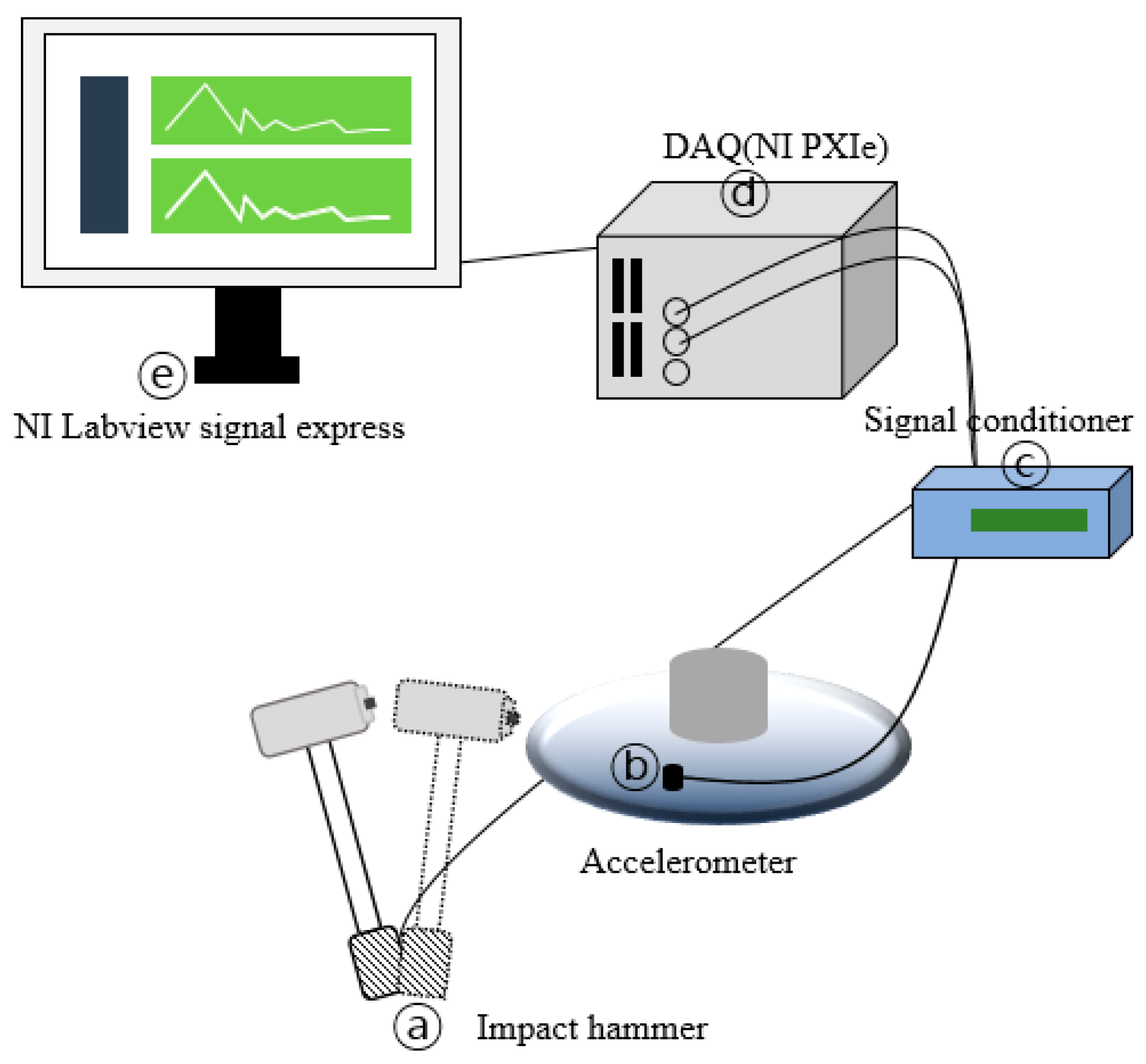
The test specimen was manufactured by NGK Ltd. in Japan, and there is a limitation for obtaining a theoretical FRF because accurate physical information is not disclosed for various variables of porcelain and cement. Therefore, FRF(H(f)) was calculated by Equation (1) using the data measured during the experiment. Equation (1) is the relationship between X(f), the power spectral density of the signal measured by an impact hammer, and Y(f), the signal cross power spectral density measured by an accelerometer.
H ( f ) = Y ( f ) X ( f ) .

2.3. Test Methods

To calculate the FRF experimentally, the impact energy and response energy must be measured. The experimental equipment was constructed as shown in Figure 2: (a) the impact hammer (PCB 086C03) was used to measure the impact energy of the specimen, (b) the accelerometer (PCB 208C05) was used to measure the response according to impact, and (c) the signal conditioner (PCB 482C16) and (d) DAQ (NI PXIe 6366) were used for data collection by the experimental equipment. The measurement program used an (e) NI Labview signal express to store the data at a sampling rate of 500 ks/s, and because the stored data were values in the time domain, they were converted to the frequency domain using the FFT using the MATLAB signal process toolbox. Next, the FRF was calculated using Equation (1).
The FRF graph according to the specimen sample is shown in Figure 3. Figure 3a is the FRF result of the normal specimens for cristobalite and alumina materials. In the graph, C1 is the result for cristobalite and A1 for alumina. Depending on the material of the porcelain insulator, the shift of the natural mode frequency was confirmed, and the alumina material had a higher natural mode than the cristobalite material. The same materials of porcelain insulators have similar FRF results, but there may be differences due to the years of use and exposure conditions. Figure 3b shows the FRF results of the normal and cracked and broken specimens. In the graph, D1 is the result for a porcelain cracked specimen and D2 for a broken disc specimen. According to the type of breakdown of the porcelain insulator, it has been confirmed that the natural mode is completely different and may vary depending on the degree of breakage. Figure 3c shows the FRF results for normal and internal defect specimens. In the graph, D3 and D4 indicate the FRF results for the specimen with internal defects. For the internal defect, a new natural mode was created at low frequencies, and some natural modes were switched to low frequencies. Additionally, porcelain insulators are used externally, so even though they are normal insulators, they show various differences in the waveform of FRF. Determination of normality and defects can be difficult because new peaks may be generated around the main peak, or other features may occur that shift some eigenmode frequencies. Through the basic FRF analysis, the characteristics of the materials and defects were identified, and based on this, the obtained data were used as basic data for feature extraction for machine learning applications.

2.4. Feature Extration

It is not appropriate to use FRF experimental data directly as the basic data for machine learning. This is because the experimental data are the energies for frequencies in the FRF graph, and although they can be compared in the natural mode as a graph when all the data are connected, not every data point with manufacturing or environmental error is significant. Therefore, feature extraction was performed to derive quantitative values from the FRF graph. The feature extraction process is shown in Figure 4, and a total of 12 features were derived using area, RMS, moment, centroid, kurtosis, and skewness; these were used as the basic dataset for machine learning. The meanings of the feature values extracted from the FRF curves are as follows: the area is the lower area of the FRF curve, root mean square (RMS) is the effective output of the FRF data, moment is the geometrical moment of area based on the origin, center is the median of the FRF curve, kurtosis is the sharpness of the FRF curve, and skewness is the degree of non-symmetry of the FRF curve.

3. Machine Learning Technique

3.1. Support Vector Machine (SVM)

In general, an SVM comprises a hyperplane or set of hyperplanes that can be used for classification or regression analysis. Intuitively, if the hyperplane has a large difference from the closest training data point, the classifier error is small; thus, a good classification requires finding the hyperplane that is farthest from the closest training data for any classified point. In general, the initial problem is dealt with in a finite dimensional space, which often results in the data not being linearly separated. To solve this problem, a method has been proposed to facilitate the separation by matching from the finite level to the higher level of the initial problem [25,29].
The linear classification using SVM is shown in Figure 5, and it is calculated as follows:
First, the given training dataset D (the set of n points) is defined as follows:
D = { ( ( x i , y i ) x i ) p , y i { 1 , 1 } } i = 1 n .
Each xi is a p-dimensional real vector, and yi is 1 or −1, indicating which class xi belongs to.
The linear separation of the above training dataset according to the value of yi is called the hyperplane and can be represented as a set of points X satisfying the following conditions:
w · x b = 0
where is the dot product, w is the normal vector of the hyperplane, and b is the deflection constant that fixes the hyperplane off-set in the p-dimensional space. The support vector ( X + ,   X ) of a given hyperplane is defined as follows:
  • X + : the data closest to the hyperplane among the data of y i = + 1 ;
  • X : the data closest to the hyperplane among the data of y i = 1 .
A hyperplane passing through X + with a legal vector equal to a given plane can be represented as w · x b = + 1 , and a hyperplane passing through X in a similar manner is represented as w · x b = 1 .
The margin of the hyperplane is the distance between the hyperplane passing through each support vector. Geometrically, the distance between two hyperplanes, or margin, is 2 w . The SVM is an algorithm that maximizes the margin.
Because there should be no data points between the hyperplanes passing through the support vector, the following equation is established:
{ w · x b + 1 ,   i f   y i = + 1 w · x b 1 ,   i f   y i = 1 .
The above two expressions can be expressed as follows:
yi ( w · x i b ) 1 ,   for   all   1 i n .
The SVM problem that follows the condition of the hyperplane and attempts to find the maximum value of the margin can be expressed as the following optimization problem:
a r g m i n w
Vapnik proposed a nonlinear classification by applying kernel tricks to the maximum margin hyperplane problem [29]. The form of the nonlinear classification algorithm is similar to the existing linear classification algorithm; however, the dot product is replaced by the nonlinear kernel function. This solves the maximum margin hyperplane problem of the transformed feature space. The transformation here may be nonlinear or may raise the dimension. That is, the classifier is a linear hyperplane in a high dimensional feature space but a nonlinear hyperplane in a conventional dimensional space. The kernel functions used for nonlinear classification are as follows [30]:
Homogeneous polynomial:
k ( x i , x j ) = ( x i · x j ) d
Polynomial kernel:
k ( x i , x j ) = ( x i · x j + 1 ) d
Gaussian radial basis function:
For γ > 0 , sometimes parametrized using γ > 1 / ( 2 σ 2 ) ,
k ( x i , x j ) = e x p ( γ x i x j 2 )
Hyperbolic tangent:
k ( x i , x j ) = t a n h ( x i · x j + c ) d
where σ is the standard deviation, γ is a constant, and d is the degree of the polynomial.
Among the SVM methods, there is an L1 regularized SVM that ignores noise features and weights only the most important features to automatically select and classify them. However, the L1 regularized SVM method can be less efficient in data analysis as the number of features that are automatically selected increases. Therefore, in this study, the PCA-SVM method, which can easily manage key factors by filtering a high amount of data in advance and has low computational effort and cost, was used [31].
The SVM model was implemented in MATLAB environment using “fitcsvm,” which trains the SVM classification model with moderate predictors. The SVM model supports the classification of predictor data using kernel functions.

3.2. Ensemble Method

An ensemble classifier was proposed to improve the classification performance of a single classifier. It combines several weak models of a single classifier to improve the machine learning results. This method was designed to solve the instability of the learning method by a single classifier, which provides better prediction performance than the single model [32,33]. The combination of a single model used in an ensemble classifier has the following methods, as shown in Figure 6.
The bagging method can generate multiple bootstraps and combine the results of each bootstrap’s prediction model to predict the results. Bagging also considers the training data as a population and obtains an average prediction model, which can reduce the variance and improve the predictive power.
The boosting method of learning ensembles can reduce the training errors rapidly and easily by combining slightly lower predictive weak classifiers, creating a single strong classifier that performs slightly better, and showing better predictive power than the bagging method by improving the predictive error.
The model joining method used in this study is a boosting method, which makes it easier and faster to build a model than other joining methods. In addition, the adaptive boosting method was used to supplement the boosting method step by step and combine them to amplify the performance of the strong classifier, and this is referred to as the Adaboost method. The Adaboost method is a sequential ensemble method in which the basic learners are created sequentially. Simple weak classifiers complement each other. In addition, the higher weighting of previously misclassified samples improves the overall performance and allows for better learning and classification by focusing on the misclassified data.

3.3. Principal Component Analysis (PCA)

Principal component analysis (PCA) reduces high-dimensional data to low-dimensional data. Orthogonal transformations are used to transform samples of a high-dimensional space that are likely to be related to each other into samples of a low-dimensional space (principal components) that have no linear correlation. The number of dimensions of the principal component is less than or equal to the number of dimensions of the original sample. PCA linearly transforms data into a new coordinate system in a manner that, when the data are mapped onto one axis, the axis with the largest variance is placed as the first principal component and that with the second largest component as the second principal component. As such, PCA is a classification method that divides the sample difference into the components that best represent the difference.

4. Analysis and Result

Twelve features extracted from the FRF graph in Figure 3 were used to construct a basic data set using PCA. As a result of the PCA, the feature value of the largest variance was the moment of real value (PC1), and the feature value of the second largest variance was the moment of imaginary value (PC2). Figure 7 shows two-dimensional scatter plots with PCs on the x-axis (PC1) and y-axis (PC2). The PCA result revealed that the normal data were distributed over a fairly wide range. This is judged to be an error that occurs because the porcelain insulators are used under various environmental conditions. Data of the broken discs were found to be outside the distribution range of the normal data, but some internal defect data were located close to the distribution range of normal data. Therefore, it is necessary to set the distribution range between normal data and porcelain damage data for these distribution results.

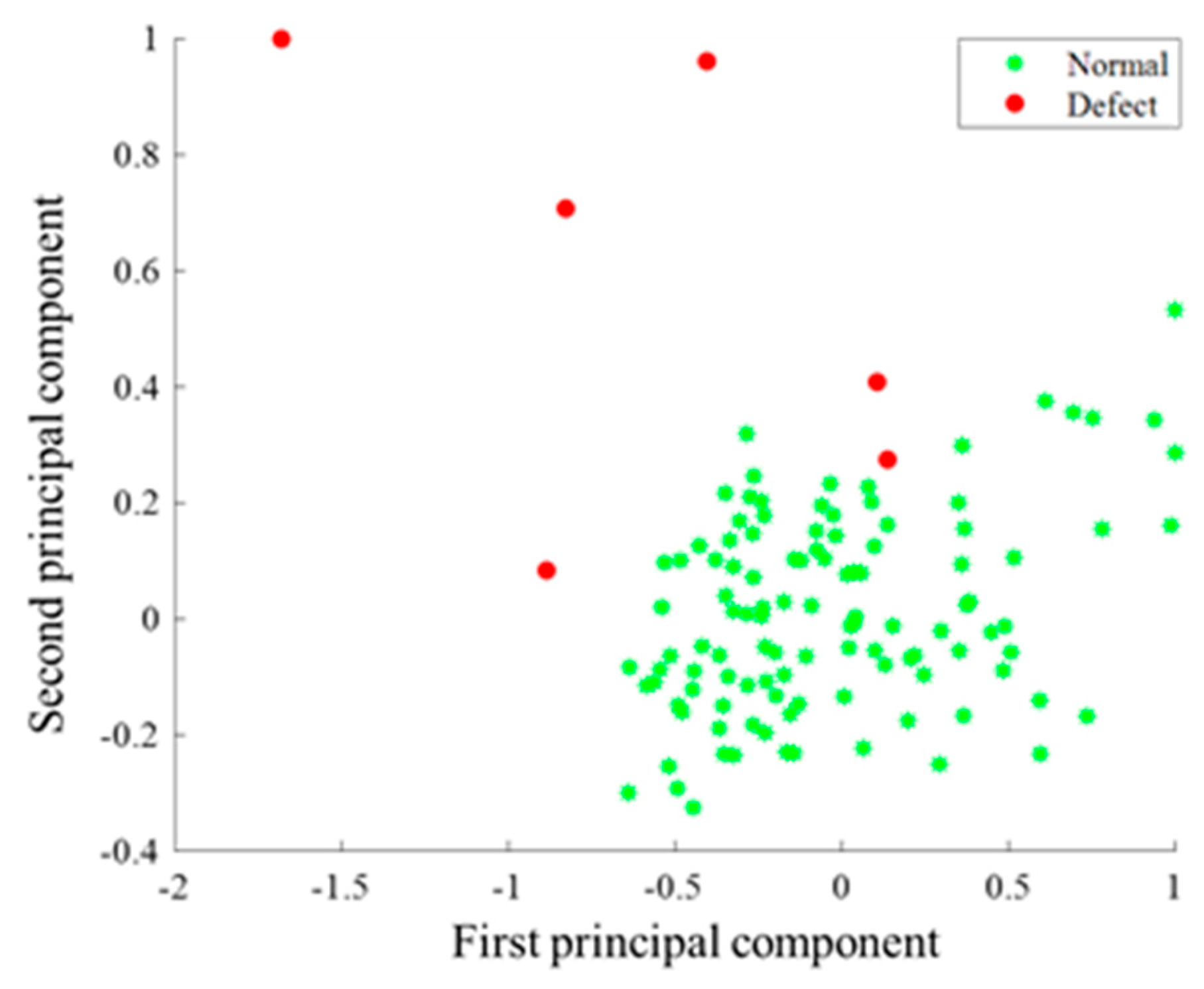
4.1. Binary Linear Separation with SVM

First, the PCA data in Figure 7 were used as the basic data for the analysis using the hyperplane, which is a linear binary classification method, among various SVM classification methods. Figure 8 shows the results divided into hyperplanes. The analysis allowed the crack and damage data of ceramics to be distinguished from the normal data, but the internal damage data and most of the normal data were distributed within the maximum margin of the hyperplane as the support vector. These results could be due to the large difference in variance between the two classes. Therefore, it is clear that linear hyperplane classification is not suitable to analyze this data.

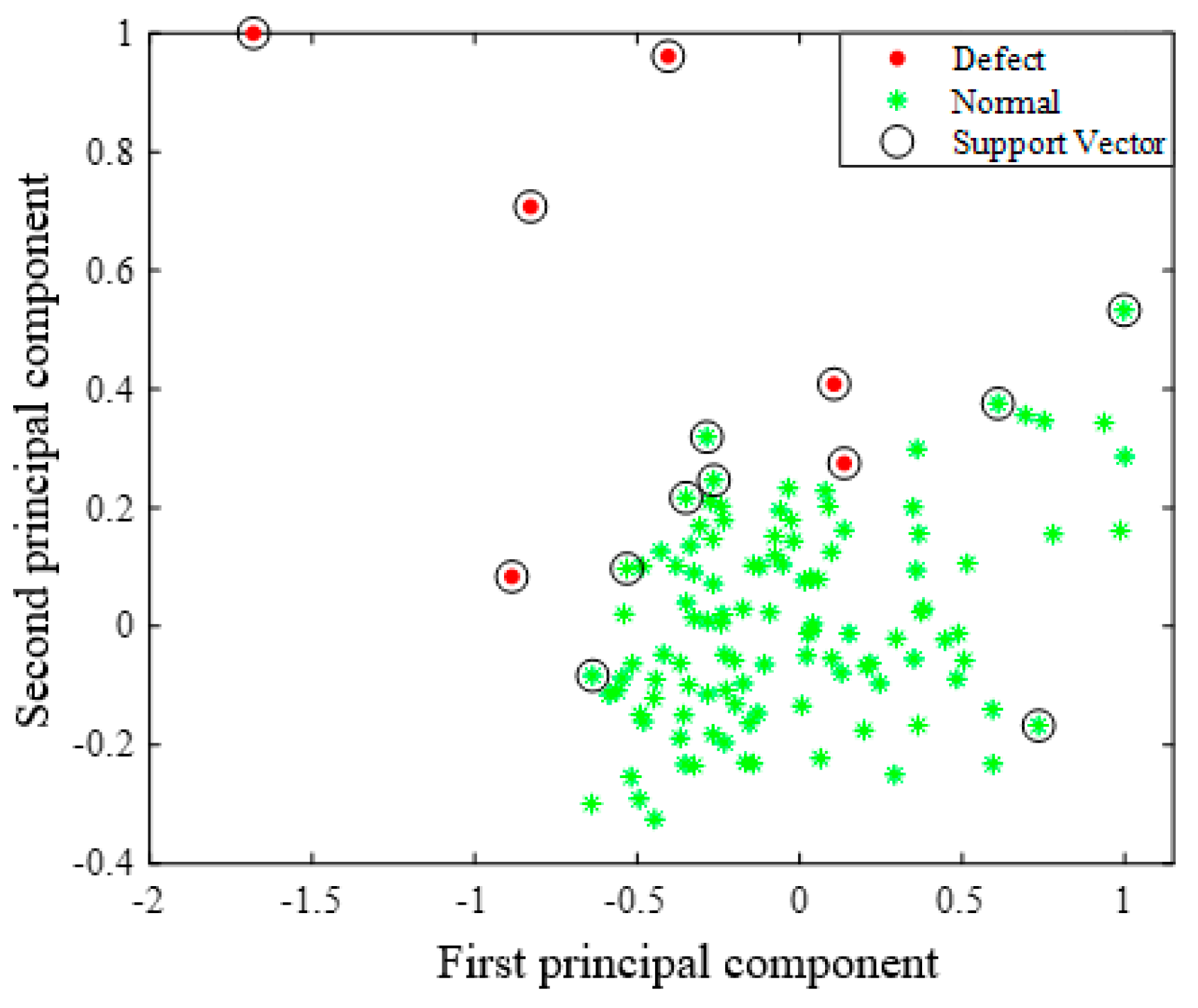
4.2. Nonlinear Separation with a Single SVM

The results of a nonlinear analysis of the normal and defective specimens using the radial basis function of the kernel function as a single SVM are shown in Figure 9.
As a result, 94 out of 111 normal data were classified as normal, but all the defect data were classified as support vectors. This indicates that they are distributed in the margin range of the boundary dividing normal and defect data. Thus, they can be defective or normal for the defect in each analysis, and it is difficult to accurately determine the data because they are separated by the boundary. Therefore, because the data classification is ambiguous, additional analysis was conducted to increase its reliability.

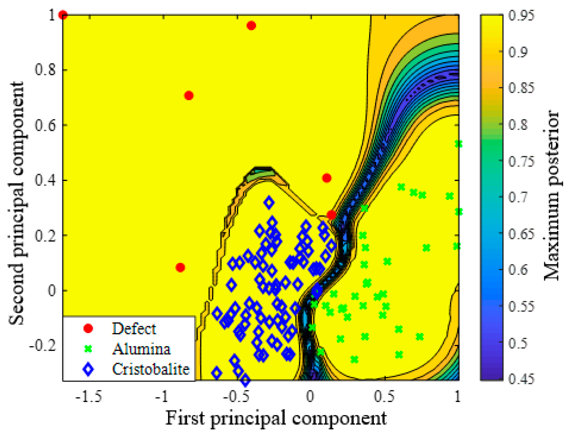
4.3. Nonlinear Separation with Multiple SVMs

Given that linear hyperplane analysis and nonlinear single SVMs are not suitable for the distribution of basic data, a nonlinear analysis was performed using multiple SVMs with the kernel function. The kernel function used was the radial basis function. When using a hyperplanar analysis and a single SVM, the classes were classified into normal and defect classes; however, in this analysis, the classes were classified into three categories: cristobalite, alumina, and defect. The SVM essentially involves binary classification; therefore, we created an individual SVM model for three classes and analyzed them through a parallel operation. Ten data points were randomly extracted and evaluated using the developed SVM model. The results are presented in Table 2. According to the criterion to classify cristobalite into cristobalite, the value of the SVM1 prediction model should be close to 1 in the three prediction models and close to 0 in the SVM2 and SMV3 models. According to the criterion for judging alumina as alumina, the value should be close to 1 in the SVM2 model and close to 0 in the SVM1 and SVM3 models. According to the criterion for determining defects as defects, the value should be close to 1 in the SVM3 model and close to 0 in the SVM1 and SVM3 models.
The post-distribution range for the entire data was calculated using the multi-SVM model, and the results are shown in Figure 10. The prediction results for these three classes are presented in Table 3. The results confirmed that most cristobalite data were distributed in the negative range based on the zero value of PC1 and that the alumina data were distributed in the positive range. Based on this, the boundary between the cristobalite and alumina data was separated with high accuracy. In addition, it was possible to set the range to accurately classify defect data and general data. However, when there is a boundary (margin) region owing to the SVM analysis characteristics, it may be difficult to determine the correct class when some data are distributed at the boundary.
The results of classifying the normal and damaged porcelain insulators using the three SVM classification methods showed that the linear hyperplane classification and the nonlinear single SVM method are not suitable for data classification in this study. In contrast, the nonlinear multiple SVM method is considered suitable for data classification. However, data exist in the boundary region owing to various errors depending on the use environment of the porcelain insulator, and it is necessary to apply another machine learning method to distinguish these data.
Therefore, an analysis was performed by applying the ensemble technique, which is used for creating a suitable model by sequentially selecting the appropriate model and assigning weights to errors in each training step.

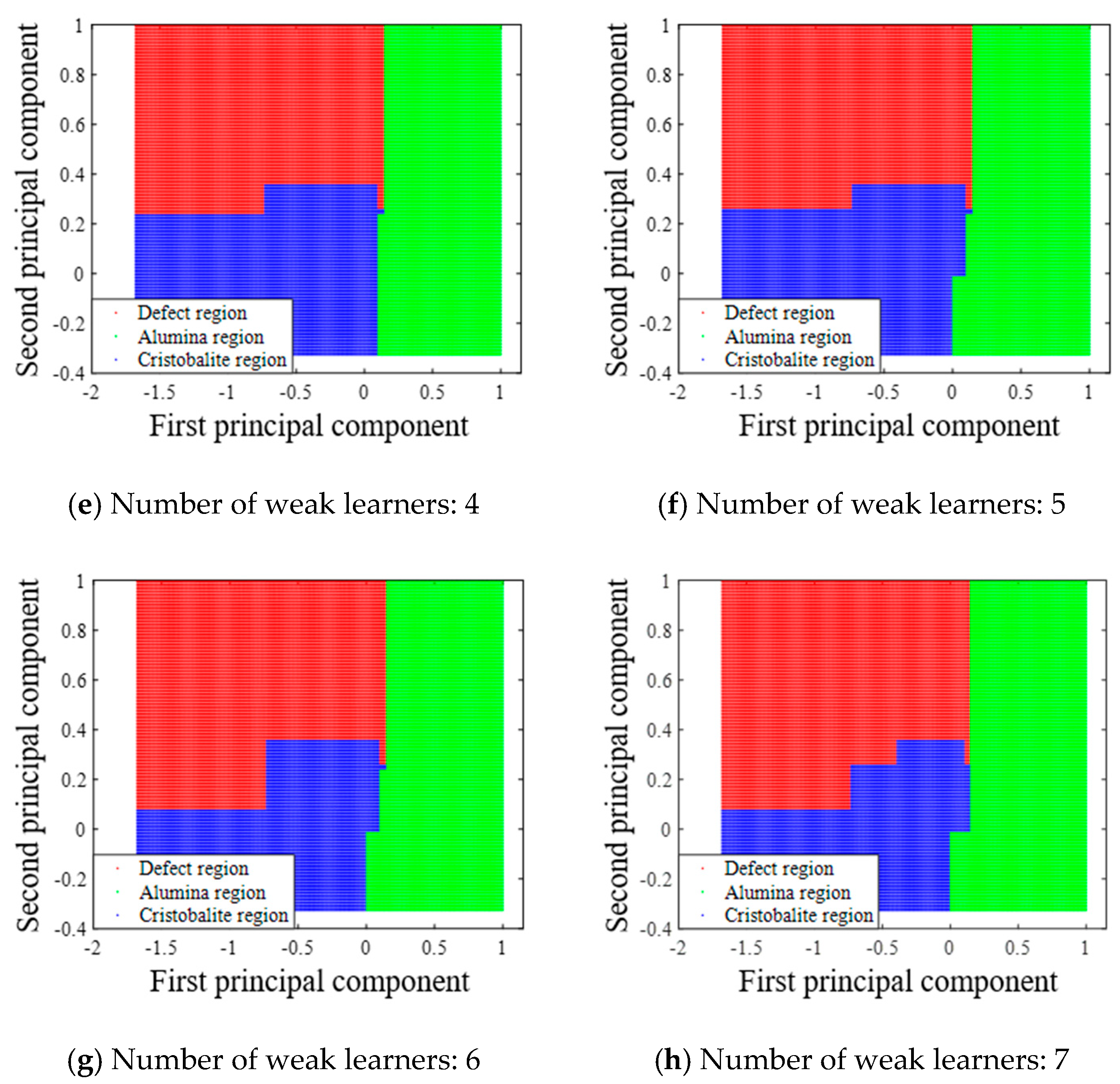
4.4. Ensemble Analysis Using Adaboost

The ensemble analysis was performed using the AdaBoost method, a type of boosting method. The ensemble analysis is a method for creating an ensemble model suitable for data classification using various weak learners. The Adaboost is a method that increases the reliability of classification through the next learner by weighting misclassification. Therefore, the optimal number of learners and the accuracy of classification were verified by increasing the number of learners. The region images for distribution of the range of data according to the ensemble analysis are shown in Figure 11. As the number of learning increased, it was possible to classify the area more accurately and precisely and predict with high accuracy. The prediction accuracy was 100% and the learning time was 0.28 s when seven learners were used. However, in the future, if a larger dataset is used, inefficiencies may occur, for example, with respect to model development time. Therefore, using the training count ratio instead of the entire dataset would increase the efficiency of prediction time and prediction degree.

5. Conclusions

A machine learning model for damage assessment of porcelain insulators using the FRF is proposed with multiple SVMs and the Adaboost ensemble method. The machine learning model for damage assessment was developed by analyzing the correlation between the extracted features, materials, and defects using the frequency response data of 117 porcelain insulators collected from 154 kV transmission towers in four regions.
  • A nonlinear classification prediction SVM model was more accurate than a linear classification one, and a combination of three nonlinear SVM models resulted in the development of the most reliable model.
  • The ensemble model could obtain more accurate prediction results than the SVM model by combining multiple single classifiers, weighting the classification result errors, and increasing the number of learners. Moreover, when seven learners were used, the prediction accuracy was the highest and the data distribution area could be finely divided.
  • The classification of porcelain damage specimens was correct; however, it could be difficult to set the division area because certain data of some internal damage specimens are close to the distribution range of normal data. Therefore, it is necessary to establish a dataset by measuring several types of defects that may occur, in order to more accurately set a damage distribution area and develop a predictive model.

Author Contributions

I.H.C., J.B.K., and J.A.S. conceived and designed the experiments; Y.G.Y. and T.K.O. performed the experiments and analyzed the data; I.H.C., J.W.W., and D.Y.B. contributed device/analysis tools; Y.G.Y. and T.K.O. wrote the paper. All authors have read and agreed to the published version of the manuscript.

Funding

This research was funded by Korea Electric Power Corporation (KEPCO). This work was supported by Research Assistance Program (2019) in the Incheon National University.

Conflicts of Interest

The authors declare that there is no conflict of interest.

References

  1. Looms, J.S.T. Introduction. In Insulators for High Voltages, 7th ed.; Peter Peregrinus Ltd.: London, UK, 1988; pp. 1–3. [Google Scholar]
  2. Vaillancourt, G.H.; Bellerive, J.P.; St-Jean, M.; Jean, C. New live line tester for porcelain suspension insulators on high-voltage power lines. IEEE Trans. Power Deliv. 1994, 9, 208–219. [Google Scholar] [CrossRef]
  3. Momen, G.; Farzaneh, M. Survey of Micro/Nano Filler Use to Improve Silicone Rubber for Outdoor Insulators. Rev. Adv. Mater. Sci. 2011, 27, 1–13. [Google Scholar]
  4. Karady, G.G.; Shah, M.; Brown, R.L. Flashover mechanism of silicone rubber insulators used for outdoor insulation. IEEE Trans. Power Deliv. 1995, 10, 1965–1971. [Google Scholar] [CrossRef]
  5. Choi, I.H.; Kim, T.K.; Yoon, Y.B.; Kim, T.Y.; Nguyen, H.T.; Yi, J.S. A Study on the Life-Time Assessment Ways and Various Failure Types of 154 kV Porcelain Insulators Installed in South Korea. Trans. Electr. Electron. Mater. 2018, 19, 188–194. [Google Scholar] [CrossRef]
  6. Bardeen, A.W.; Sheadel, J.M. Corrosion as it affects insulator and conductor hardware. In Proceedings of the AIEE Winter General Meeting, New York, NY, USA, 30 January–3 February 1956; pp. 491–501. [Google Scholar]
  7. Cavallini, A.; Chandrasekar, S.; Montanari, G.C.; Puletti, F. Inferring ceramic insulator pollution by an innovative approach resorting to PD detection. IEEE Trans. Dielectr. Electr. Insul. 2007, 14, 23–29. [Google Scholar] [CrossRef]
  8. Vaillancourt, G.H.; Carignan, S.; Jean, C. Experience with the detection of faulty composite insulators on high-voltage power lines by the electric field measurement method. IEEE Trans. Power Deliv. 1998, 13, 661–666. [Google Scholar] [CrossRef]
  9. Padma, V.; Raghavan, V.S. Analysis of insulation degradation in Insulators using Partial Discharge analysis. In Proceedings of the 2011 3rd International Conference on Electronics Computer (ICECT), Kanyakumari, India, 8–10 April 2011; pp. 110–114. [Google Scholar]
  10. Cherney, E.A.; Am, D.E. Development and application of a hot-line suspension insulator tester. IEEE Trans. Power Appar. Syst. 1981, 4, 1525–1528. [Google Scholar] [CrossRef]
  11. Ha, H.; Han, S.; Lee, J. Fault detection on transmission lines using a microphone array and an infrared thermal imaging camera. IEEE Trans. Instrum. Meas. 2012, 61, 267–275. [Google Scholar] [CrossRef]
  12. Miao, X.R.; Liu, X.Y.; Chen, J.; Zhuang, S.B.; Fan, J.W.; Jiang, H. Insulator Detection in Aerial Images for Transmission Line Inspection Using Single Shot Multibox Detector. IEEE Access 2019, 7, 9945–9956. [Google Scholar] [CrossRef]
  13. Jeon, S.H.; Kim, T.Y.; Lee, Y.J.; Shin, J.J.; Choi, I.H.; Son, J.A. Porcelain Suspension Insulator for OHTL: A Comparative Study of New and Used Insulators using 3D-CT. IEEE Trans. Dielectr. Electr. Insul. 2019, 26, 1654–1659. [Google Scholar] [CrossRef]
  14. Ryder, S.A. Diagnosing transformer faults using frequency response analysis. IEEE Electr. Insul. Mag. 2003, 19, 16–22. [Google Scholar] [CrossRef]
  15. Christain, J.; Feser, K. Procedures for detecting winding displacements in power transformer by the transfer function method. IEEE Trans. Power Deliv. 2004, 19, 214–220. [Google Scholar] [CrossRef]
  16. Miyazaki, S.; Mizutani, Y.; Matsumoto, K.; Nakamura, S. On-Site Diagnosis of Transformer Winding by Frequency Response Analysis. IEEJ Trans. Power Energy 2010, 130, 451–459. [Google Scholar] [CrossRef]
  17. Miyazaki, S.; Mizutani, Y.; Taguchi, A.; Murakami, J.; Tsuji, N.; Takashima, M.; Kato, O. Diagnosis Criterion of Abnormality of Transformer Winding by Frequency Response Analysis (FRA). Electr. Eng. Jpn. 2017, 201, 25–34. [Google Scholar] [CrossRef]
  18. Miletiev, R.; Simeonov, I.; Iontchev, E.; Yordanov, R. Time and frequency analysis of the vehicle suspension dynamics. Int. J. Syst. Appl. 2013, 7, 287–294. [Google Scholar]
  19. Li, J.C.; Dackermann, U.; Xu, Y.L.; Samali, B. Damage identification in civil engineering structures utilizing PCA-compressed residual frequency response functions and neural network ensembles. Struct. Control Health Monit. 2011, 18, 207–226. [Google Scholar] [CrossRef]
  20. Kim, Y.S.; Shong, K.M.; Jeon, Y.J. A Study on the site vibration for the breakage analysis of glass insulators on the high-speed railway. IEEE Trans. Power Deliv. 2009, 24, 1809–1814. [Google Scholar] [CrossRef]
  21. Pearson, K. On lines and planes of closest fit to systems of points in space. Lond. Edinb. Dublin Philos. Mag. J. Sci. 1901, 2, 559–572. [Google Scholar] [CrossRef] [Green Version]
  22. Zhang, G.; Tang, L.Q.; Zhou, L.C.; Liu, Z.J.; Liu, Y.P.; Jiang, Z.Y. Principal Component Analysis Method with Space and Time Windows for Damage Detection. Sensors 2019, 19, 2521. [Google Scholar] [CrossRef] [Green Version]
  23. Raghu, S.H.; Sriraam, N.J. Classification of focal and non-focal EEG signals using neighborhood component analysis and machine learning algorithms. Expert Syst. Appl. 2018, 113, 18–32. [Google Scholar] [CrossRef]
  24. Mantero, P.; Moser, G.; Serpico, S.B. Partially supervised classification of remote sensing images through SVM-based probability density estimation. IEEE Trans. Geosci. Remote Sens. 2005, 43, 559–570. [Google Scholar] [CrossRef]
  25. Burges, C.J.C. A tutorial on support vector machines for pattern recognition. Data Min. Knowl. Discov. 1998, 2, 121–167. [Google Scholar] [CrossRef]
  26. Rokach, L. Taxonomy for characterizing ensemble methods in classification tasks: A review and annotated bibliography. Comput. Stat. Data Anal. 2009, 53, 4046–4072. [Google Scholar] [CrossRef] [Green Version]
  27. Hsieh, S.L.; Hsieh, S.H.; Cheng, P.H.; Chen, C.H.; Hsu, K.P.; Lee, I.S.; Wang, Z.; Lai, F. Design Ensemble Machine Learning Model for Breast Cancer Diagnosis. J. Med. Syst. 2011, 36, 2841–2847. [Google Scholar] [CrossRef] [PubMed]
  28. ES (Technical Standards of KEPCO). Testing Methods for Insulators; Korea Electric Power Corporation: Daejeon, Korea, 2014. [Google Scholar]
  29. Vapnik, V.; Cortes, C. Support-vector networks. Mach. Learn. 1995, 20, 273–297. [Google Scholar]
  30. Kavzoglu, T.; Colkesen, I. A kernel functions analysis for support vector machines for land cover classification. Int. J. Appl. Earth Obs. Geoinformation 2009, 11, 352–359. [Google Scholar] [CrossRef]
  31. Benkaddour, M.K.; Bounoua, A. Feature extraction and classification using deep convolutional neural networks, PCA and SVC for face recognition. Traitement du Signal 2017, 34, 77–91. [Google Scholar] [CrossRef]
  32. Hansen, L.K.; Salamon, P. Neural network ensembles. IEEE Trans. Pattern Anal. Mach. Intell. 1990, 10, 993–1001. [Google Scholar] [CrossRef] [Green Version]
  33. Freund, Y.; Schapire, R.E. A decision-theoretic generalization of on-line learning and an application to boosting. J. Comput. Syst. Sci. 1997, 55, 119–139. [Google Scholar] [CrossRef] [Green Version]
Figure 1. Sketch of porcelain insulator showing possible defects.
Applsci 10 00084 g001
Figure 2. The frequency response function (FRF) test method.
Applsci 10 00084 g002
Figure 3. FRF results and images of materials and defective specimens. (a) FRF results and images of normal specimens, (b) FRF results and images of specimens with porcelain defects, and (c) FRF results and images of specimens with internal defects.
Applsci 10 00084 g003
Figure 4. Feature extraction from the FRF of experimental data.
Applsci 10 00084 g004
Figure 5. Binary linear separation with a support vector machine (SVM).
Applsci 10 00084 g005
Figure 6. Procedure for developing ensemble models using weak learners.
Applsci 10 00084 g006
Figure 7. Scatter plot of PC1 and PC2.
Applsci 10 00084 g007
Figure 8. Binary linear hyperplane separation with the SVM.
Applsci 10 00084 g008
Figure 9. Nonlinear separation with a single SVM using kernel function.
Applsci 10 00084 g009
Figure 10. Nonlinear separation with multiple SVMs using kernel function.
Applsci 10 00084 g010
Figure 11. Results of ensemble classification according to the increase in the number of learners.
Applsci 10 00084 g011aApplsci 10 00084 g011b
Table 1. Categorization of specimens according to type of material and defects.
CategorizationCristobaliteAluminaSum
Total8037117
Normal7437111
Defect typeSub total6-6
Porcelain4-4
Internal2-2
Table 2. Prediction values by nonlinear separation with multiple SVMs.
True LabelPredict LabelPosterior
SVM1SVM2SVM3
Alumina‘Alumina’0.10430.89550.0002
Cristobalite‘Cristobalite’0.99900.00010.0009
Cristobalite‘Cristobalite’0.99930.00060.0001
Cristobalite‘Cristobalite’0.99930.00020.0005
Alumina‘Alumina’0.00000.98990.0101
Cristobalite‘Cristobalite’0.99920.00000.0008
Alumina‘Alumina’0.00000.99360.0063
Defect‘Defect’0.05890.01160.9295
Cristobalite‘Cristobalite’0.99860.00030.0011
Table 3. Prediction ratio by nonlinear separation with multiple SVMs.
TypeCristobaliteAluminaDefectBoundary
Cristobalite72 (97.3%)--2 (2.7%)
Alumina-36 (97.3%)-1 (2.7%)
Defect--6 (100%)-

