Article

A New Online Operational Modal Analysis Method for Vibration Control for Linear Time-Varying Structure

1
College of Computer Science and Technology, Huaqiao University, Xiamen 361021, China
2
State Key Laboratory for Strength and Vibration of Mechanical Structures, Xi’an Jiaotong University, Xi’an 710049, China
3
College of Mechanical Engineering and Automation, Huaqiao University, Xiamen 361021, China
4
Department of Mathematics and Statistics, San Diego State University, San Diego, CA 92182, USA
*
Author to whom correspondence should be addressed.
Appl. Sci. 2020, 10(1), 48; https://doi.org/10.3390/app10010048
Submission received: 1 November 2019 / Revised: 13 December 2019 / Accepted: 16 December 2019 / Published: 19 December 2019
(This article belongs to the Section Acoustics and Vibrations)

Abstract

:
From the viewpoint of vibration control, if the amplitude of the main frequencies of the vibration response can be reduced, the vibration energy of the structure is greatly reduced. Modal parameters, including modal shapes, natural frequencies, and damping ratios, can reflect the dynamics of the structure and can be used to control the vibration. This paper integrates the idea of “forgetting factor weighting” into eigenvector recursive principal component analysis, and then proposes an operational modal analysis (OMA) method that uses eigenvector recursive PCA with a forgetting factor (ERPCAWF). The proposed method can identify the transient natural frequencies and transient modal shapes online and realtime using only nonstationary vibration response signals. The identified modal parameters are also suitable for online, real-time health monitoring and fault diagnosis. Finally, the modal identification results from a three-degree-of-freedom weakly damped linear time-varying structure shows that the ERPCAWF-based OMA method can effectively identify transient modal parameters online using only nonstationary response signals. The results also show that the ERPCAWF-based approach is faster, requires less memory space, and achieves higher identification accuracy and greater stability than autocorrelation matrix recursive PCA with a forgetting factor-based OMA.

1. Introduction

During the production and use of a structure, vibration is inevitable. Vibration can cause damages to the structure and endanger human health [1]. The aim of operational modal analysis (OMA) is to identify the modal parameters (modal frequencies, mode shapes, and mode damping ratios) of structures by analyzing only their vibration response signals under operating conditions, rather than in a laboratory environment [2]. Recently, this technology has become an important method for solving vibration problems in engineering and has been widely used in mechanics, especially in the aerospace, civil engineering, maritime navigation, railway, and heavy equipment industries [3,4].
A linear structure whose system parameters (i.e., mass, stiffness, or damping) change over time is called a linear time-varying (LTV) structure. Ramnath [5] defined a system that has much less variation in its coefficients than its solutions as a slow linear time-varying (SLTV) system. Currently, there are two main modal parameter identification studies related to LTV structures [6]. The first one is based on the time–frequency analysis of nonstationary response signals [7], including the wavelet transform [8], Hilbert–Huang transform [9], and so on. The second category is the time domain method, which can be divided into time-varying state-space model-based method [10] and time-varying autoregressive moving average model-based approaches [11]. In time domain and (time–)frequency methods, the identification of time-varying structures is achieved by “short time invariant”-based method [12] and online and recursive techniques. Under the assumption of “short time invariant”, and the theories of “time-freezing” [13] and “quasi-stationary” systems, the non-stationary response signals can be regarded as stationary response time series and the LTV structures can be regarded as linear time invariant (LTI) structures over short periods of time. A representative method is the moving window technique [14]. In online and recursive techniques, when identifying newly added data, it is not necessary to re-create a new model, and only the old model is required to recursively obtain the model at this moment. The core of online and recursive techniques is the recursive algorithm. However, in recursive methods, old data, which are not relevant at the time of study, still have a large impact on the results. Therefore, forgetting factor is introduced to solve this problem.
In methods based on time–frequency analysis, vibration signals are processed offline in a batch-wise manner rather than online and recursively, so the wavelet transform- and Hilbert–Huang transform-based methods cannot be applied to online vibration control, structural health diagnosis, and realtime damage detection [15,16]. The “short time invariant”-based methods are computationally expensive, and their results may be somewhat delayed and only applicable to SLTV structures. These online and recursive techniques have the problems of low precision and high time and space complexity, which means it takes a lot of time and space storage to execute these algorithms and the newest acquisition signal may not to be processed in a timely manner. The complexity of the algorithm has a great impact on its performance [17,18,19]. Therefore, this article is dedicated to reducing space and time complexity and improving identification accuracy.
PCA is a multivariate statistical technique that has been successfully applied to fault diagnosis [20], the monitoring of industrial processes [21], and operational modal parameter identification in mechanical structures [22,23]. By applying PCA, several principal components that reflect the essential vibrational characteristics of the system are extracted from highly correlated data. In modal analysis, PCA is sometimes called proper orthogonal decomposition (POD) [24]. There exists a one-to-one relationship between the modal shapes of dynamic mechanical systems and the linear compound matrix, and a one-to-one relationship between the modal coordinate responses and principal components (PCs) [25]. This hypothesis has been confirmed also in [26,27].
However, classical PCA or POD models are batch-wise multivariate statistical methods that are only suitable for stationary signals. In other words, they are time-invariant and cannot identify the operational modal parameters of LTV structures. Recently, some adaptive PCA methods have been developed for nonstationary signal processing. In [28], Wold combined an exponentially weighted moving average with PCA. The moving window PCA method combats the time-varying nature of the structural parameters using a fixed-length window. A PCA model is established in the old moving window and reconstructed in the new window each time a new data sample is received [29]. Therefore, this method is computationally expensive and memory-intensive. Recursive PCA (RPCA) employs a recursive technique to update the reference model for every new sample [30]. Depending on the required parameters (autocorrelation matrix and eigenvector), multiple RPCA algorithms may be used, such as autocorrelation matrix RPCA (ARPCA) [31] and eigenvector RPCA (ERPCA) [32]. Most RPCA techniques are based on updating a rank-one matrix. As a result, RPCA increasingly includes old data and cannot represent the current features. This problem can be solved by introducing a forgetting factor to reduce the impact of old data.
Guan et al. [33] developed a limited memory PCA (LMPCA)-based OMA method to identify both the modal shapes and frequencies of SLTV structures. However, this method has a long runtime, high memory requirements, pathological matrix problems, and suffers from modal exchange. To reduce the runtime and memory requirements of LMPCA-based OMA, Wang et al. [34] proposed an OMA method based on limited memory autocorrelation matrix RPCA. This method updates the autocorrelation matrix in every moving window, rather than rebuilding the PCA model. Therefore, the computation time and memory requirements of LMRPCA-based OMA are much less than moving window PCA-based OMA. To avoid pathological matrix problems, Zhang et al. [35] described a new OMA method using moving window self-iteration principal component extraction (MWSIPCE). However, these moving window-based methods have an inherent delay and should be confined to SLTV structures. Guan et al. [36] developed an ARPCA with a forgetting factor (ARPCAWF) for OMA, and identified transient modal parameters for a beam with time-varying density by updating the autocorrelation matrix online. This method is suitable for both SLTV and fast linear time-varying (FLTV) structures, but suffers from pathological matrix problems and modal exchange, and has high computation times and memory requirements.
In this paper, an ERPCA with a forgetting factor (ERPCAWF) based OMA method for the online identification of transient modal parameters in weakly damped LTV structures is considered. ERPCA uses all of the old data and a rank-one matrix to update the eigenvalue and eigenvector. This eigenvector corresponds to the modal shape vector. However, the presence of old data makes it difficult to extract the current features. Thus, a forgetting factor is introduced to reduce the weight of the old data. In our method, the forgetting factor has a fixed value; determining this value according to the time-varying speed of the structures remains an open problem. In addition, the proposed method is currently confined to LTV structures.
In summary, our contributions are as follows:
  • We simplify the model and coefficients, and describe a transient representation of LTV structures. Furthermore, we design the steps of the PCA-based OMA vibration control method to reduce amplitude of the vibration response.
  • We analyze the disadvantages of PCAWF- and ARPCAWF-based OMA for LTV structures, such as the high time complexity, space complexity, time required for matrix decomposition, modal exchange, and low accuracy.
  • Integrating the idea of “forgetting factor weighting” and the technology of ERPCA, we propose an ERPCAWF-based OMA method to identify the transient natural frequencies and transient modal shapes of LTV structures using only nonstationary response signals under unmeasured stationary ambient loads. This method is suitable for both SLTV and FLTV structures.
  • Through a theoretical comparison among different adaptive PCA-based OMA methods, we show that ERPCAWF-based OMA offers a faster runtime, lower memory consumption, and comparable accuracy while avoiding the ill-posed, singular values of matrix decomposition and modal exchange problems. By enhancing the efficiency and stability of modal parameter identification for LTV structures, this method is more suitable for online, real-time health monitoring and fault diagnosis.
  • We analyze the limitations and application scope of ERPCAWF-based OMA for LTV structures.
  • We design a three degree-of-freedom (DOF) weakly damped LTV structure to verify the operational modal identification ability of ERPCAWF-based OMA. A comparison of different methods using nonstationary vibration response simulation data shows that ERPCAWF-based OMA is faster, less memory-intensive, and more precise than the ARPCAWF-based OMA method.
This paper is organized as follows. In Section 2, we introduce the transient representation of LTV structures. In Section 3, we describe PCAWF- and ARPCAWF-based OMA for SLTV structures and analyze their limitations. The proposed ERPCAWF-based OMA technique is illustrated in Section 4, and the operational modal identification ability of ERPCAWF-based OMA is verified in Section 5. Finally, we conclude this paper in Section 6.

2. Transient Representation of LTV Structures

Different from the theory behind frozen-in coefficients, operational modal parameter identification in the transient representation of LTV structures can be described as follows.

2.1. Dynamics of N-DOF LTV Structures

The dynamic characteristics of a system are an intrinsic property that reflects the linear relationship between the inputs and outputs of the system. Common engineering structures are usually regarded as having proportional viscous damping. Based on the theory of structural dynamics, the equation of motion in an N-DOF LTV vibrating structure is [37]:
M ( t ) X ¨ ( t ) + C ( t ) X ˙ ( t ) ( t ) + K ( t ) X ( t ) = F ( t ) , t [ t b e g i n , t e n d ]
where M ( t ) , C ( t ) , and K ( t ) R N × N are the time-varying mass, damping, and stiffness matrices, respectively; X ¨ ( t ) ) , X ˙ ( t ) , and X ( t ) R N × T are the acceleration, velocity, and displacement matrices, respectively; and F ( t ) R N × T is the excitation matrix.

2.2. Modal Coordinate Decomposition of Vibration Response in N-DOF LTV Structures

As the mass, stiffness and damping of the system are time-varying, the transient natural frequencies and modal shapes, as for a linear system there are N modes, are different at each moment. However, at time t, for real modal analysis in the modal coordinate, the vibration response signals of weakly damped mechanical structures can be decomposed into the inner product of the modal shapes matrix and the modal responses matrix:
X ( t ) = Φ ( t ) Q ( t ) = k = 1 N φ k ( t ) q k ( t )
where X ( t ) is the output displacement; Φ ( t ) R N × N is the time-varying transient modal shape matrix composed of transient modal shapes φ k ( t ) R N ; and Q ( t ) = [ q 1 ( t ) , q 2 ( t ) , , q k ( t ) , , q N ( t ) ] T is the matrix composed of modal responses q k ( t ) from each mode. Based on linear systems vibration theory, when the time-varying transient natural frequencies f k ( t ) of each mode are not equal, the vectors of the time-varying transient main modes φ k ( t ) are orthogonal.
Φ T ( t ) M ( t ) Φ ( t ) = M r ( t ) = d i a g [ m 1 ( t ) , m 2 ( t ) , , m k ( t ) , , m N ( t ) ] Φ T ( t ) K ( t ) Φ ( t ) = K r ( t ) = d i a g [ k 1 ( t ) , k 2 ( t ) , , k k ( t ) , , k N ( t ) ]
The modal response vectors q k ( t ) are then independent of each other, and Q ( t ) satisfies:
Q ( t ) Q ( t ) T = Λ N × N ( t ) = α 1 ( t ) 0 0 0 α k ( t ) 0 0 0 α N ( t )
where Λ N × N ( t ) is a time-varying real positive diagonal matrix.

2.3. PCA-Based OMA Method for Vibration Control

Principal component analysis (PCA) can be used to identify the modal parameters of a structure [25]. The modes that PCA can recognize from the vibration response are sorted from the largest to the smallest in terms of vibrational energy. The modal shapes and modal frequencies that contribute greatly are identified and their different contribution rates can be calculated. This concept has important practical significance for the design of active and passive vibration damping optimization. It can not only determine the main modes to be optimized, but also grasp the main weak links and take relevant measures (for example, increasing the modal damping of the main contribution modes or using the actuator to actively suppress the vibration of the main contribution modes). In addition, model simplification can be performed based on the main contribution modes for online modeling and control, and the damping effect achieved by optimization can be estimated. Therefore, the further research direction is to combine the PCA-based modal parameter identification technique with the active and passive vibration reduction optimization design. The steps are shown in Figure 1.
In the process of optimization design of active and passive vibration reduction, the modal shape and modal frequency of the main contribution of the vibration system are constantly changing. To ensure real-time performance and effect, it is necessary to perform online PCA modeling and modal contribution analysis.

3. PCAWF- and ARPCAWF-Based OMA Methods and Their Limitations

PCAWF- and ARPCAWF-based OMA can identify the transient natural frequencies and transient modal shapes using only nonstationary vibration response signals from LTV structures under unmeasured stationary ambient loads. Through the introduction of forgetting factors, the relationship between the new data and the old data are taken into account in the nonstationary response signals of LTV structures.

3.1. Theory of PCAWF

When a linear structure is time-varying, its vibration response signals under operating conditions (unmeasured ambient loads) are nonstationary; the transformation matrix and PC matrix obtained from the PCA model are also time-varying. The basic principle of PCAWF is that the newly added data and the historical data matrix are assigned different weighting factors. The newly added data should have a higher weight to better characterize the newest state. The historical data matrix should be assigned a lower weight to reduce the influence of these data on the newest processing data matrix. There are many different ways of assigning the weighting factors, such as the radiation weighting factor [38], tissue weighting factor [39], and normalized weighting factor [40] techniques. In this paper, we describe the exponential forgetting factor as an example. Figure 2 illustrates the principle of the exponential forgetting factor algorithm.
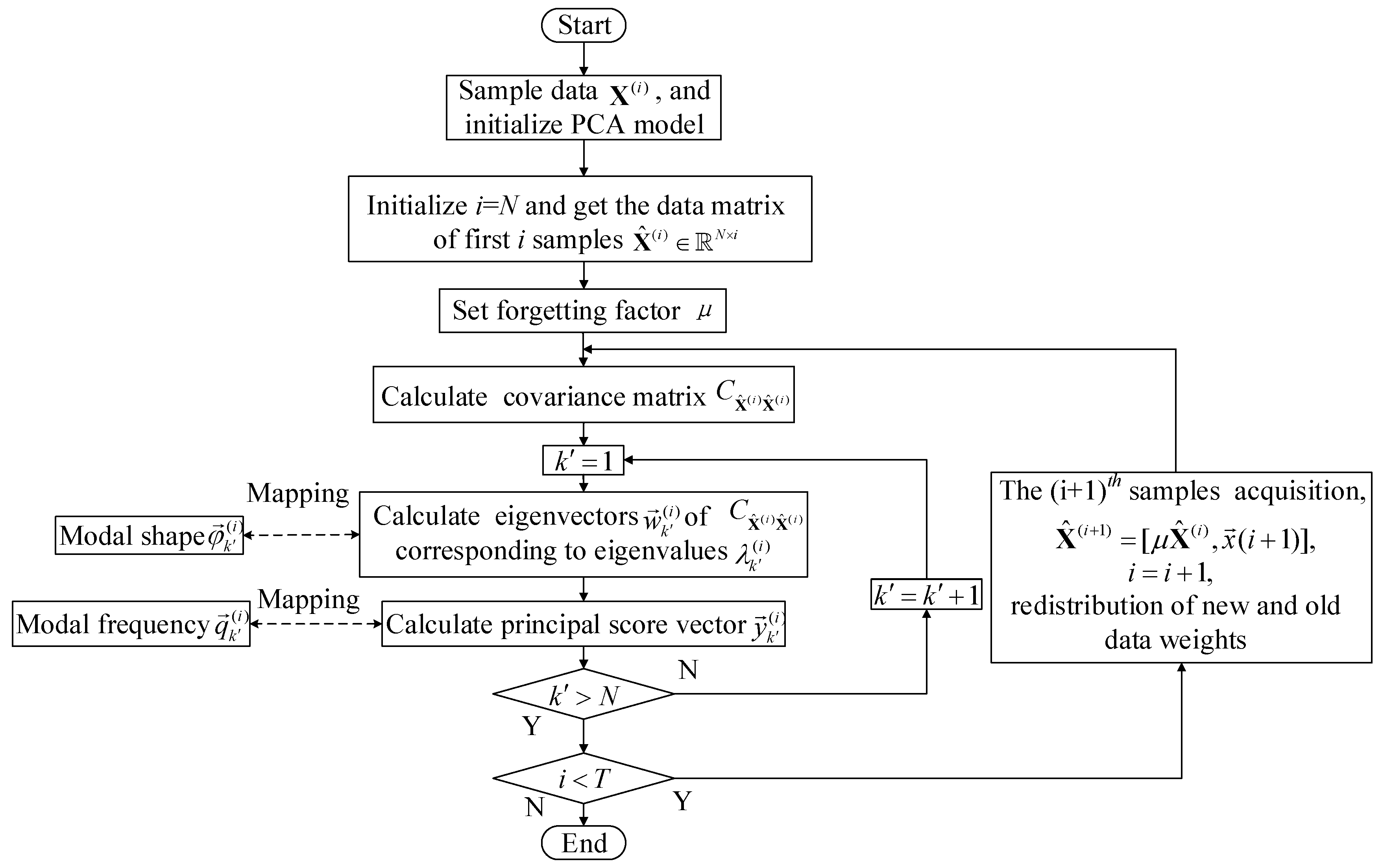
Specifically, in Figure 2, X ^ ( i ) R N × i is the weighted data. The blue curves represent the weight of each column of data, ranging from 0 to 1. As new data are added, the number of data columns increases and the weight of old data decreases. The range of the exponential forgetting factor μ is [0, 1] and the newest time data vector is assumed to have the unit weight. The previous data are then weighted according to X ^ ( i + 1 ) = [ μ X ^ ( i ) , x ( i + 1 ) ] . Thus, the weighted data matrix for the PCAWF model is as follows:
X ^ ( 1 ) = [ x ( 1 ) ] X ^ ( 2 ) = [ μ X ^ ( 1 ) , x ( 2 ) ] = [ μ x ( 1 ) , x ( 2 ) ] X ^ ( 3 ) = [ μ X ^ ( 2 ) , x ( 3 ) ] = [ μ 2 x ( 1 ) , μ x ( 2 ) , x ( 3 ) ] X ^ ( i ) = [ μ X ^ ( i 1 ) , x ( i ) ] = [ μ ( i 1 ) x ( 1 ) , μ ( i 2 ) x ( 2 ) , μ ( i 3 ) x ( 3 ) , , x ( i ) ] X ^ ( i + 1 ) = [ μ X ^ ( i ) , x ( i + 1 ) ] = [ μ ( i ) x ( 1 ) , μ ( i 1 ) x ( 2 ) , μ ( i 2 ) x ( 3 ) , , x ( i + 1 ) ] X ^ ( T ) = [ μ X ^ ( T 1 ) , x ( T ) ] = [ μ ( T 1 ) x ( 1 ) , μ ( T 2 ) x ( 2 ) , μ ( T 3 ) x ( 3 ) , , μ ( T i 1 ) x ( i + 1 ) , , x ( T ) ]
where i is the time step, x ( i ) is the data vector from time step i, and X ^ ( i ) is the data matrix of the first i samples.
The PCAWF model takes its transformation matrix and PC matrix from the weighted data matrix X ^ ( i ) rather than the original data matrix X ( i ) . A larger μ can bring the average weight closer between the new data and old data. If μ = 1 , then X ^ ( i ) = X ( i ) and the PCAWF model reduces to the PCA model. Furthermore, smaller values of μ better reflect the newest state of the system and indicate that the algorithm has good tracking performance. However, the value of μ should not be too small, otherwise it will increase the sensitivity of the estimated parameters. The forgetting factor μ should be selected using prior knowledge of the time-varying speed of LTV structures. A fast time-varying speed requires a large forgetting factor. Similar to the window size in a moving window approach, the forgetting factor is a tuning parameter that varies depending on how quickly the normal process changes [31].

3.2. Theory of ARPCAWF

In classical PCA, X ( i ) R N × i is a data matrix of N variables and i samples. This matrix can be decomposed as follows:
X ( i ) W ( i ) Y ( i )
where W ( i ) R N × M and Y ( i ) R M × i are the transformation matrix and PC matrix, respectively, and M is the number of PCs. The correlation matrix C X ( i ) X ( i ) R N × N can be written as:
C X ( i ) X ( i ) 1 i 1 X ( i ) X ( i ) T = W ( i ) Λ ( i ) W ( i ) T
where the columns of W ( i ) are the eigenvectors of C X ( i ) X ( i ) corresponding to the M largest eigenvalues, and Λ ( i ) R M × M is a real positive diagonal matrix corresponding to the M largest eigenvalues.
The classical PCA or PCAWF model is a batch-wise statistical method. When a new sample becomes available, the autocorrelation matrix or transformation matrix and the PC matrix of PCA/PCAWF need to be recalculated. In RPCA methods, the autocorrelation matrix or transformation matrix and PC matrix of PCA/PCAWF are updated recursively. Various recursive methods can be employed for this purpose, such as autocorrelation matrix recursion, eigenvector recursion [32], rank-1 corrected recursion [41], and subspace tracking recursion [42]. In this section, we describe how a weighting factor is introduced into the recursive autocorrelation calculations. The forgetting factor will have a significant effect on the statistical properties of the model output. Let us assume that the row mean vector b X ( i ) R N × 1 , data matrix X ( i ) , and auto-correlation matrix C X ( i ) X ( i ) R N × N have been calculated using the first i samples. b x j ( i ) denotes the jthrow of b X ( i ) . Thus, the recursive calculations for the mean vector b X ( i + 1 ) , standard deviation vector σ X ( i + 1 ) , and C X ( i + 1 ) X ( i + 1 ) are:
b x j ( i + 1 ) = μ b x j ( i ) + ( 1 μ ) x j ( i + 1 ) , j = 1 , , N
σ 2 x j ( i + 1 ) = μ { σ 2 x j ( i ) + [ b j ( i + 1 ) ] 2 } + ( 1 μ ) [ x j ( i + 1 ) b x j ( i + 1 ) ] 2
C X ( i + 1 ) X ( i + 1 ) = μ Σ i + 1 1 [ Σ i C X ( i ) X ( i ) Σ i + b ( i + 1 ) b T ( i + 1 ) ] Σ i + 1 1 + ( 1 μ ) x ( i + 1 ) x T ( i + 1 )
where b j ( i + 1 ) = b x j ( i + 1 ) b x j ( i ) , b ( i + 1 ) = b X ( i + 1 ) b X ( i ) R N × 1 , Σ i + 1 = d i a g { σ x 1 ( i + 1 ) , , σ x N ( i + 1 ) } R N × N , and 0 < μ i i + 1 < 1 is the forgetting factor. When μ = i i + 1 , the ARPCAWF model reduces to the ARPCA model. Therefore, the transformation matrix can be obtained by decomposing the autocorrelation matrix in Equation (7) and the PCs can be calculated using Equation (6).

3.3. PCAWF-Based OMA for LTV Structures

We now construct a PCAWF-based OMA method for LTV structures using the principle of the exponential forgetting algorithm (Equation (5)) combined with PCA-based OMA for LTI structures. The principles of modal parameter recognition are as follows: (1) Data from the first i samples are selected to initialize the PCA model and the exponential forgetting factor is set to μ . Different weights are assigned to the columns of the initial data matrix. (2) The PCA-based OMA method for LTI structures is used to find the modal parameters (instantaneous modal frequency and modal shape) at time step i. (3) When the time step ( i + 1 ) vibration response vector is added, the matrix of the previous ( i + 1 ) samples vibration response matrix is reassigned with a different weight. The PCA model is reconstructed to determine the instantaneous modal parameters. (4) The instantaneous modal parameters identified at each time are connected using a curve fitting technique, allowing the modal parameters to be identified and the LTV structure to be tracked. The procedure of PCAWF-based OMA for LTV structures is illustrated in Figure 3.

3.4. ARPCAWF-Based OMA for LTV Structures

Similar to Equations (6) and (7), X ( i + 1 ) and C X ( i + 1 ) X ( i + 1 ) can be decomposed as follows:
X ( i + 1 ) W ( i + 1 ) Y ( i + 1 )
C X ( i + 1 ) X ( i + 1 ) = W ( i + 1 ) Λ ( i + 1 ) W ( i + 1 ) T
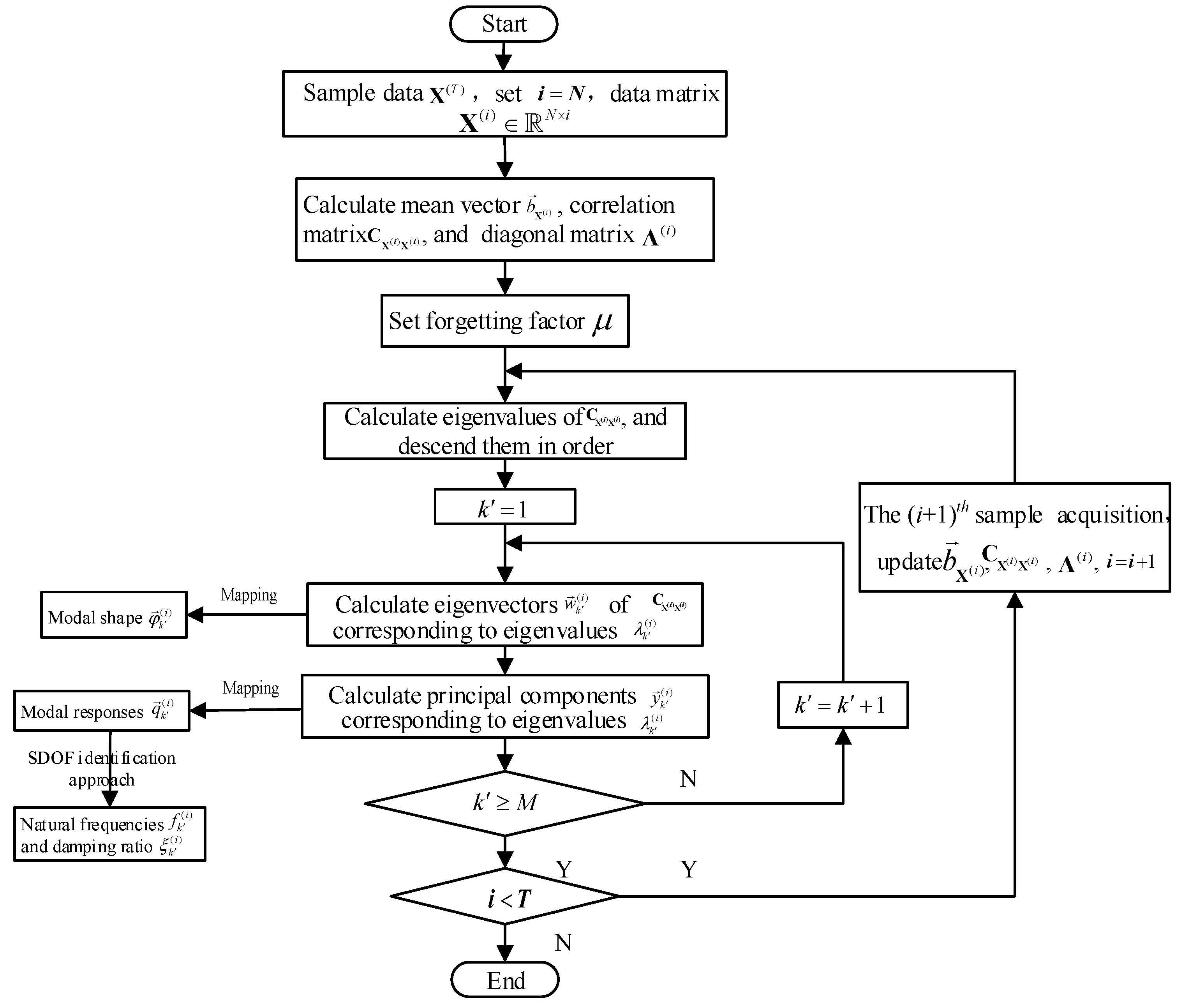
where W ( i + 1 ) R N × M and Y ( i + 1 ) R M × ( i + 1 ) are the transformation matrix and PC matrix of time step ( i + 1 ) , respectively, and the columns of W ( i + 1 ) are eigenvectors of C X ( i + 1 ) X ( i + 1 ) corresponding to the M largest eigenvalues. The eigenvectors W ( i + 1 ) of C X ( i + 1 ) X ( i + 1 ) correspond to the modal shapes, and the PC matrix Y ( i + 1 ) corresponds to the modal responses Q ( i + 1 ) . The procedure of ARPCAWF-based OMA for LTV structures is illustrated in Figure 4.

3.5. Limitations of PCAWF and ARPCAWF-Based OMA for LTV Structures

  • When the PCA models are updated using the PCAWF or ARPCAWF algorithm, the PCs and eigenvectors must be calculated through matrix decomposition, which is computationally expensive. Furthermore, the algorithm process requires several large matrices to be stored, and these occupy a large amount of memory. Therefore, PCAWF- and ARPCAWF-based OMA methods have high time and space complexity.
  • In the process of dealing with the observed data, the results are always sensitive to observation noise. In the field of mathematics, this is known as an ill-posed problem [43], and matrix decomposition is particularly susceptible to such issues. In practical engineering applications, the crux of solving ill-posed problems is to replace the matrix decomposition method [44]. When a new data vector is added to the PCAWF model, there is a serious risk that the updated matrix will be ill-posed. This may result in biased matrix decomposition, inaccurate PCs and eigenvectors, and poor adaptive PCAWF-based OMA.
  • As ARPCAWF recursively updates the autocorrelation matrices rather than all PCA models, it has lower time and space complexity than PCAWF. For the autocorrelation covariance matrix, the recursive solution of the modal parameters requires repeated recursive computations to determine the covariance matrix at the next moment, which consume a lot of time and occupies large amounts of memory. For the PCA solution, if the variance of a variable changes, the characteristic structure of the covariance matrix decomposition will change completely, affecting the load vector assignment. If the mean value of the variable changes, the PC orientation will deviate. However, the PCs and eigenvectors are also calculated by matrix decomposition, thus the problems of matrix decomposition persist.
  • PCAWF- and ARPCAWF-based OMA suffer from the problem of modal exchange. For LTV structures, the engineering parameters (mass, stiffness, and damping) change over time, thus the order of each modal contribution rate may vary. Because of this modal exchange, the contribution order is not equal to the frequency order. The modal exchange phenomenon will cause the eigenvalues in the PCA decomposition results to be similar or even the same, and the PCA method based on singular value decomposition or eigenvalue decomposition appears singular or ill-conditioned, leading to a reduction in the accuracy of recognition results or even wrong results [34]. However, the order of the mode identified by PCA depends on its contribution rather than its frequency. In PCAWF- and ARPCAWF-based OMA, the eigenvectors and PCs are calculated by eigenvalue decomposition or singular value decomposition of the autocorrelation matrix and re-ordered according to the associated eigenvalues.

4. ERPCAWF-Based OMA Method for LTV Structures

In the process of time-varying structural changes, older data samples will eventually be unable to characterize the newest state of the current time-varying system. Thus, in describing the current state of the system, it becomes necessary to consider the weights of the older and newer data samples. In this paper, we integrate the idea of “forgetting factor weighting” into ERPCA to give the proposed ERPCAWF. The exponential forgetting factor method is used to determine the proportion of historical data and newer data used in the real-time updating of the entire PCA model. Furthermore, the modal parameters for LTV structures are extracted by recursively updating the PCA model. Ultimately, this achieves the purpose of real-time online identification.

4.1. Theory of ERPCAWF

To avoid recalculating the PCs and eigenvectors by matrix decomposition, we use a rank-1 matrix to correct the error [39], and update the new PCs and eigenvectors according to the eigenvalues and eigenvectors from the previous step. This realizes the effective tracking of time-varying structures. The rank-1 correction can be described as:
C r a n k 1 = D r a n k 1 + ε u u T
where C r a n k 1 R N × N and D r a n k 1 R N × N are diagonal matrices with diagonal elements c k and d k ( k = 1 , 2 , , N ) , respectively, and ε is a constant. u R N × 1 is the newest data vector, and C r a n k 1 R N × N is calculated by correcting D r a n k 1 R N × N according to the diagonal matrix u u T . This is called rank-1 matrix correction because the rank of u R N × 1 is 1.
Let the covariance matrix at time step i, C X ( i ) X ( i ) be able to be decomposed into C X ( i ) X ( i ) = W ( i ) Λ ( i ) W ( i ) T , where Λ ( i ) is a real positive diagonal matrix and W ( i ) R N × N is the unit orthogonal matrix. Thus, Equation (13) becomes:
C X ( i + 1 ) X ( i + 1 ) = μ W ( i ) Λ ( i ) W ( i ) T + ( 1 μ ) x ( i + 1 ) x T ( i + 1 ) = W ( i ) [ μ Λ ( i ) + ( 1 μ ) ( W ( i ) T ) x ( i + 1 ) ( W ( i ) T x T ( i + 1 ) ) ] W ( i ) T = W ( i ) ( D r a n k 1 + ε u u ) W ( i ) T
Let D r a n k 1 = μ Λ ( i ) , ε = 1 μ , u = W ( i ) T x ( i + 1 ) . Then, through rank-1 correction, we obtain:
P Γ P T = μ Λ ( i ) + ( 1 μ ) ( W ( i ) T x ( i + 1 ) ) ( W ( i ) T x ( i + 1 ) ) T
Equation (14) can be further simplified as:
C X ( i + 1 ) X ( i + 1 ) = W ( i ) P Γ PW ( i ) T
where W i + 1 = W ( i ) P and Λ ( i + 1 ) = Γ is the diagonal matrix formed by the updated eigenvalues. Therefore,
C X ( i + 1 ) X ( i + 1 ) = W ( i + 1 ) Λ ( i + 1 ) W ( i + 1 ) T
where W ( i + 1 ) is the updated eigenvector. Thus, the sub-vector of the updated PC is:
Y ( i + 1 ) = W ( i + 1 ) T X ( i + 1 )
Therefore, the new PCs and eigenvectors will be updated according to the old eigenvalues and eigenvectors on every iteration.

4.2. ERPCAWF-Based OMA for LTV Structures

Using the covariance matrix recursively to identify and track the modal parameters of LTV structures has a certain flaw. Therefore, in ERPCAWF-based OMA, the rank-1 correction method is introduced to modify the autocorrelation matrix. In fact, because the updates do not destroy the PCA model, the eigenvalues, eigenvectors, and PCs are updated directly. The eigenvectors correspond to modal shapes and the PCs correspond to the modal response matrix. The proposed ERPCAWF-based OMA method directly obtains the modal parameters for each update. A curve fitting technique is used to connect the modal parameters identified at each moment, enabling modal parameter identification and the tracking of the LTV structure. The procedure of ERPCAWF-based OMA is illustrated in Figure 5.

4.3. Performance Analysis of ERPCAWF-Based OMA and Its Advantages

Obtaining the eigenvectors and PCs via recursive method directly places lesser computational and memory requirements on ERPCAWF-based OMA. In other words, the algorithm is more suitable for integration into embedded devices. For PCAWF, we must update all PCA models, then calculate the autocorrelation matrix, and finally compute the PCs and eigenvectors by decomposing the autocorrelation matrix, resulting in high overall time and space complexities. ARPCAWF-based OMA recursively updates the autocorrelation matrices rather than all the PCA models. This means that ARPCAWF-based OMA has lower time and space complexities than PCAWF-based OMA, but is still more computationally expensive than ERPCAWF-based OMA.
As matrix decomposition is only performed at the start of the calculation process, ERPCAWF-based OMA faces few problems with ill-posed matrices. However, both PCAWF- and ARPCAWF-based OMA perform matrix decomposition T times, so there is potential for many ill-posed problems to occur. Thus, ERPCAWF-based OMA may achieve higher accuracy than PCAWF- and ARPCAWF-based OMA.
There are many different adaptive PCA-based OMA methods that use only nonstationary vibration response signals from LTV structures under unmeasured stationary ambient loads. Table 1 compares several such methods in terms of their time complexity, space complexity, modal exchange, number of matrix decompositions, accuracy, and applicability. L denotes the length of the moving window, r denotes the number of iterations, and M is the number of principal components to be extracted.

4.4. Limitations and Application Scope of ERPCAWF-Based OMA for LTV Structures

The proposed ERPCAWF-based OMA for LTV structures has the following limitations:
(1) Each order of modal shapes obtained by PCA is ortho-normalized, resulting in the loss of amplitude information. This is a characteristic of PCA-based OMA, and is retained in ERPCAWF-based OMA for LTV structures. The order of the modes identified by PCA depends on their contribution, rather than their frequency values. Hence, modal deletion may occur when a mode makes only a small contribution.
(2) The forgetting factor is selected through prior knowledge of the time-varying speed of the LTV structure. However, the forgetting factor should be fully self-adaptive, with the ability to change according to the nonstationary vibration response signals when there is no prior knowledge of the time-varying speed.
(3) PCA-based OMA methods can identify mode shapes, modal frequencies, and mode damping ratios for LTI structures using only stationary vibration response signals. The proposed ERPCAWF method for OMA can also identify time-varying transient mode shapes, modal frequencies, and mode damping ratios from non-stationary vibration response signals. However, theoretical analysis and numerical simulations indicate that a decreasing or moving mass will generate additional damping [45,46] in the LTV structure. The time-varying transient mode damping ratio identified by ERPCAWF cannot be compared with the mode damping ratio calculated by finite element methods.
The scope of application of the proposed ERPCAWF-based OMA for LTV structures is as follows:
(1) For real modal analysis in the modal coordinates, the vibration response signals of weakly damped mechanical structures can be decomposed into the inner product of the modal shapes matrix and modal responses matrix. This method is only suitable for the real modal identification of linear and weakly damped structures. When the damping is too large, the modal parameter identification for LTV structures will entail complex modal analysis and complex parameter identification.
(2) The proposed method is suitable for both SLTV and FLTV structures. However, ERPCAWF-based OMA is currently confined to LTV structures [47] and is unsuitable in scenarios where modal jumping phenomena may occur [48,49].

5. Simulations

5.1. Description of LTV Three-DOF System

Numerical simulation experiments were conducted with a three-DOF time-varying mass. The test system defined is the same as that used in Ref. [36]. The equations of motion for systems with time-varying mass can be written as Equation (19):
m 1 ( t ) 0 0 0 m 2 ( t ) 0 0 0 m 3 ( t ) x 1 ¨ x 2 ¨ x 3 ¨ + c 1 + c 2 c 2 0 c 2 c 2 + c 3 c 3 0 c 3 c 3 x 1 ˙ x 2 ˙ x 3 ˙ + k 1 + k 2 k 2 0 k 2 k 2 + k 3 k 3 0 k 3 k 3 x 1 x 2 x 3 = F 1 ( t ) 0 0
In this example, we consider a system with mass m 1 ( t ) = 1 kg for 0 t 50 s and m 1 ( t ) = e 0.00005 ( t 50 ) for 50 t 2000 s. m 2 ( t ) = m 3 ( t ) = 1 kg, stiffness k 1 ( t ) = k 2 ( t ) = k 3 ( t ) = 1000 N/m, and damping c 1 ( t ) = c 2 ( t ) = c 3 ( t ) = 0.01 Ns/m for 0 t 2000 s. The external force F ( t ) = [ F 1 ( t ) 0 0 ] T is white noise excitation with zero mean and unit variance. Figure 6 shows the three-DOF system model with external excitation.
The dynamic response was acquired using the n e w m a r k β method. The simulation had a sampling time of 2000 s and sampling frequency of 40 Hz. All experiments were conducted on a server running Microsoft Windows 10 64-bit with four CPUs and 32 GB memory. MATLAB version 2016a was used to run the simulations and multiple variable memories were pre-allocated.

5.2. Theoretical Mode Solution

As the linear structure has a time-varying quality, its transient natural frequencies and modal shapes are evolving. However, at time t, the mass, stiffness, and damping can be considered to be determined. Therefore, it is possible to find the transient modal natural frequencies and modal shapes at that time, as for LTI structures.
The simulation results were verified against the actual modes of the weakly damped structure. According to the theory and finite element analysis, all of the natural frequencies are undamped and the modal shapes are real. According to vibration dynamics theory, the frequencies and modal shapes can be computed using the secular equation:
K w k 2 M = 0
where K , M R N × N are the stiffness and mass matrices, respectively, and w k is the eigenvalue of Equation (20) corresponding to the k th natural frequency. The eigenvector φ k corresponding to the k th natural frequency and w k is the k th mode shape, which satisfies:
( K w k 2 M ) φ k = 0
The modal damping ratio is defined as:
ξ k = c k 2 w k m k
where the modal mass matrix M r , modal stiffness matrix K r , and modal damping matrix C r satisfy:
K r = M r Λ = M r w 1 2 0 0 0 w k 2 0 0 0 w N 2
where Φ = [ φ 1 , φ 2 , , φ k , , φ N ] is the modal shape matrix.

5.3. Modal Assurance Criterion

To determine the accuracy of the modal shapes, the modal assurance criterion (MAC) is introduced to verify the operational modal identification results. The MAC is given by [50]:
M A C φ i , ϕ j = ( φ i T ϕ j ) 2 ( φ i T φ i ) ( ϕ j T ϕ j )
where φ i is the ith identified modal shape, ϕ j is the jth theoretical modal shape, and φ i T and ϕ j T are the transpositions of φ i and ϕ j , respectively. The MAC values range between 0 (no coincidence) and 1 (complete coincidence). However, MAC only reveals information about the direction and shape of the modal results, and does not contain any information about the modal amplitudes. The MAC value is always 1 if the two vectors are proportional. In this paper, the modal shapes recognition results of various methods are compared with the modal shapes obtained from theoretical analytical solutions through calculating the MAC values to verify the accuracy.

5.4. LTV Three-DOF Simulation Results

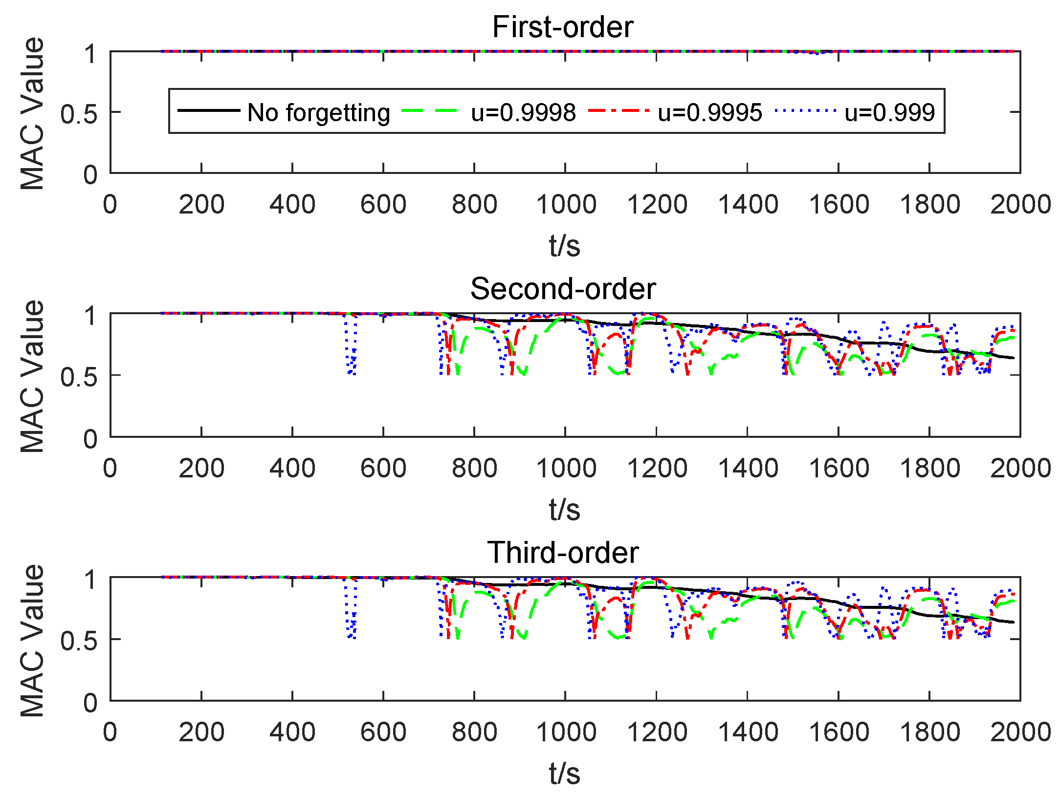
The simulation results given by the proposed ERPCAWF technique are now presented. The first-order recognition results of PCA-based OMA methods are the results of most energetic mode, which corresponds to the first mode (sorted by natural frequency) in this simulation. The variation in the MAC value under different forgetting factors is shown in Figure 7.
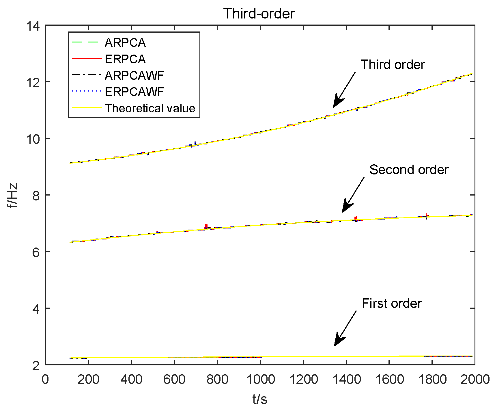
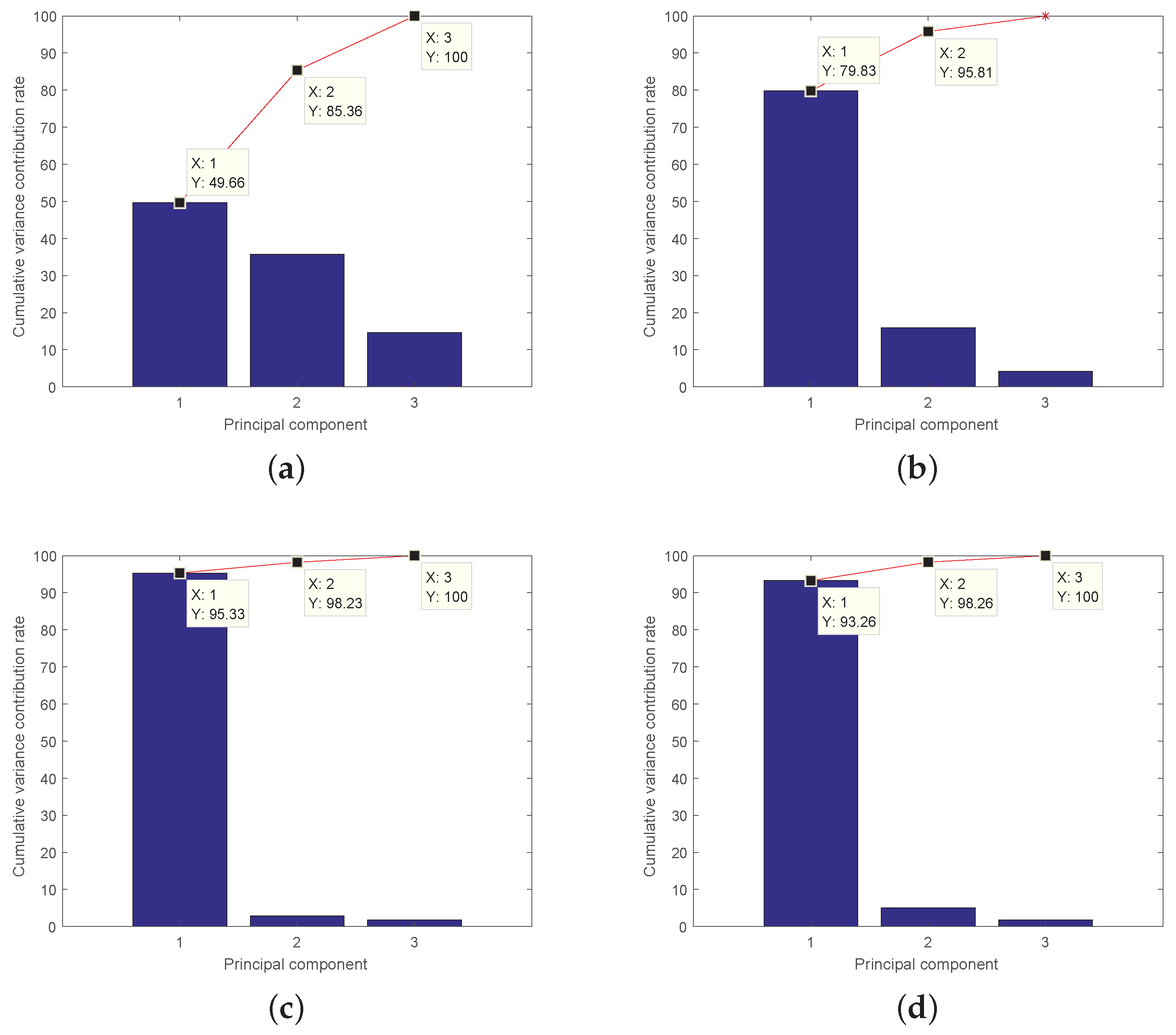
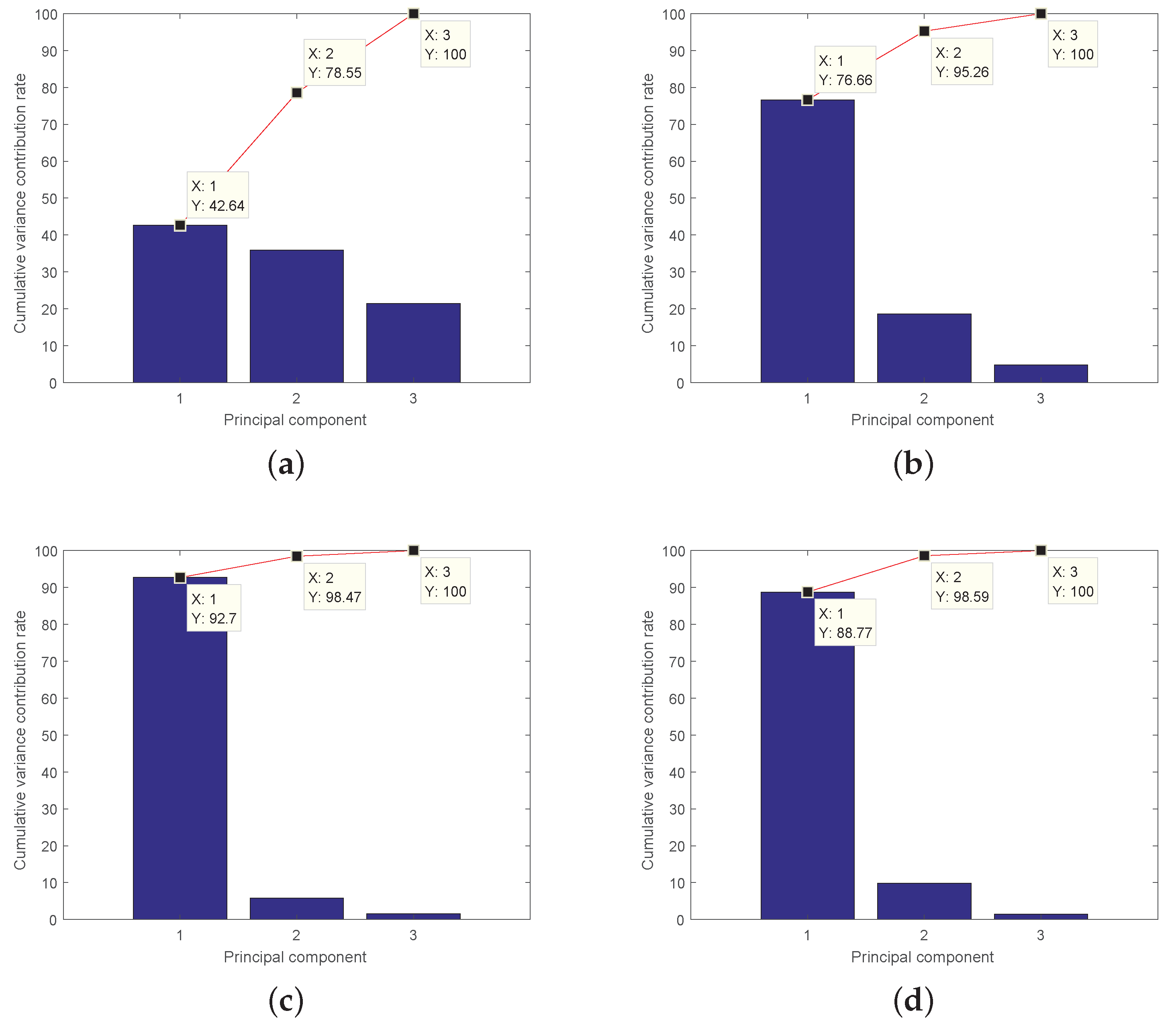
In Figure 7, we calculate the mean value of the MAC of four methods from 1250 to 2000 s. Then, by calculating, the mean value of the third-order MAC value results when μ = i i + 1 (without forgetting factor), μ = 0.9998 , μ = 0.9995 , and μ = 0.9990 are 0.8511, 0.7983, 0.8347, and 0.8653, respectively. Therefore, the best identification results obtained when μ = 0.9990 . Furthermore, when the forgetting factor is not used, the accuracy of recognition decreases over time. With μ = 0.9990 , the modal natural frequencies identified by ERPCAWF, ARPCAWF, ARPCA, ERPCA, and theoretical calculations are shown in Figure 8. To better compare the frequency identification results, Figure 9 describes the relative errors of the four methods. The relative error calculation process is: calculate the absolute value of the theoretical value and the identification value, and then divide it by the theoretical value. The modal shapes results of ARPCAWF-, ARPCA-, ERPCA- and ERPCAWF-based OMA are compared with the theoretical modal shapes to calculate the MAC values, which is shown in Figure 10. Figure 11 and Figure 12 present the contribution of each PC to the variance at different randomly selected moments (112.75, 581.4, 1275.3, and 1987.25 s) for the ERPCAWF- and ARPCAWF-based techniques, respectively. In Figure 11 and Figure 12, the blue histogram is the variance contribution rate and Y coordinate value is the cumulative variance contribution rate. The cumulative variance contribution rate indicates the proportion of all the currently selected principal components carrying information of the original data. The results given by ERPCAWF-, ERPCA-, ARPCA- and ARPCAWF-based OMA at these moments are listed in Table 2. Recall that the MAC value reflects the accuracy of modal shape identification [51]. To obtain the time and space requirements, for each algorithm, we ran 100 times and calculated the average. Table 3 compares the time and space complexities of the different algorithms.

5.5. Analysis of Modal Identification Results

(1) For the LTV three-DOF system considered in the simulations, Figure 7 clearly shows that different forgetting factors have an effect on the recognition of the modal shape for ERPCAWF-based OMA method. The current choice of forgetting factor is not a uniform standard, and is mostly based on empirical choice. In this study, the recognition results under different forgetting factors were compared. After 1250 s, the best forgetting factor that makes the experimental structure is 0.9990.
(2) With μ = 0.9990 , Figure 8 shows that ERPCAWF-based OMA can effectively identify and track frequency changes in the time-varying system. This further validates the ERPCAWF-based OMA method. In Figure 8 and Figure 9, we can see that the natural frequencies can be well identified by ERPCAWF-, ARPCAWF-, ARPCA-, and ERPCA-based OMA methods. The results seem to be exactly the same between the methods because the three-DOF system in Figure 6 is a slow time-varying system and the natural frequencies do not change much (first order is 0.0697 Hz, second order is 0.9460 Hz, and third order is 3.1748 Hz). In addition, the natural frequencies are calculated by picking the peaks of the Fourier transform of the latest 4096 modal coordinate responses, instead of picking the peaks of the Fourier transform of all the identified modal coordinate responses.
(3) Figure 10 and Table 2 show that the ERPCAWF-based OMA method achieves a high MAC value, which means that this approach can effectively identify the modal shapes of LTV structures. ERPCAWF-based OMA offers higher precision than ARPCAWF-based OMA. The time-varying system changes quickly at some time steps and slowly at some time steps. In Figure 10, ERPCA looks more stable than ERPCAWF, because the the forgetting factor in ERPCAWF is fixed ( μ = 0.9990 ). To make ERPCAWF-based OMA stable, a variable forgetting factor that can self-adaption change related to the time-varying speed characteristics of vibration signals is needed.
(4) As shown in Figure 11 and Figure 12, for LTV structures, the engineering parameters (mass, stiffness, and damping) change over time, thus the modal contribution rate of each order varies with time. The contribution order is not the same as the frequency order, and the correspondence between the two rankings may change over time. This phenomenon is called modal exchange. In Figure 7, each modal shape identified by ERPCAWF corresponds to the theoretical value. By avoiding the modal exchange phenomenon, the ERPCA- and ERPCAWF-based OMA methods offer greater stability than ARPCA- and ARPCAWF-based OMA in vibration control [34,36].
(5) From the results in Table 3, we can confirm that ERPCAWF-based OMA has a shorter runtime and requires less memory than ARPCA-, ERPCA-, and ARPCAWF-based OMA method. Our method can quickly identify modal parameters and apply them to online vibration control.
(6) In Table 2 and Table 3, the differences between ERPCA and ERPCAWF are very small. In Table 2, due to the data length, 112.5 s is the first data matrix and their identified results are the same at this time. ERPCA- and ARPCA-based OMA methods are only suitable for LTI system. In other word, with the increase of time, the ERPCA- and ARPCA-based OMA method cannot keep up with the change of system modal shapes, which leads to the decrease of MAC recognition accuracy. The difference between ERPCA and ERPCAWF is the value of μ ; their space-time complexities are the same in theory and very close in simulation results. Therefore, in Table 3, the time and space requirements for ERPCA and ERPCAWF are close. The same is true for ARPCA and ARPCAWF.

6. Conclusions and Prospects

This paper describes a method that combines the idea of “forgetting factor weighting” with eigenvector recursive PCA. The proposed eigenvector recursive PCA with a forgetting factor enables innovative operational modal parameter identification for LTV structures. Because the eigenvalues and eigenvectors of the autocorrelation matrix destroy the PCA model, a rank-1 matrix is used to correct the errors. The new PCs and eigenvectors are updated according to the eigenvalues and eigenvectors from the previous step, allowing ERPCAWF-based OMA to identify the transient modal parameters for LTV structures. This paper also describes the steps to control vibration using modal parameters. Simulation results demonstrate that the ERPCAWF-based OMA method has the advantages of faster run time, lower memory space requirements, higher identification accuracy, and greater stability than PCAWF- and ARPCAWF-based OMA. Our approach can identify modal parameters quickly and accurately, and further apply them to solving vibration control problems.
However, this research also has some limitations. The value of forgetting factor has a great influence on the accuracy of recognition results. If no forgetting factor is added, the recognition accuracy gradually decreases. Therefore, how to set the self-adaptive selection of forgetting factors based on the time-varying speed characteristics of vibration signals is our future research direction. Before being applied to engineering applications, ERPCAWF-based OMA should be verified under different types of ambient excitation, time-varying speed especially fast linear time-varying, more complex three-dimensional engineering structures, online health monitoring, and fault diagnosis. Identifying the damping ratio of LTV structures will be addressed in subsequent studies.

Author Contributions

Conceptualization, C.W. and X.L.; Data curation, C.W.; Formal analysis, C.W., H.H. and X.L.; Funding acquisition, C.W. and H.H.; Investigation, C.W., H.H. and X.L.; Methodology, C.W. and H.H.; Project administration, C.W. and J.C.; Resources, C.W. and X.L.; Supervision, C.W., X.L., and J.C.; Validation, C.W., H.H., and J.C.; Visualization, C.W. and H.H.; Writing—original draft, C.W., H.H., and X.L.; and Writing—review and editing, C.W., H.H., and J.C. All authors have read and agreed to the published version of the manuscript.

Funding

This work was financially supported by the National Natural Science Foundation of China (Nos. 51305142, 51305143, 18BTJ031 and 71571056), Postgraduate Scientific Research Innovation Ability Training Plan Funding Projects of Huaqiao University (No. 17013083018), the Quanzhou Science and the Technology Plan (No. 2018C110R) and the National Science Foundation (No. DMS-0907710).

Conflicts of Interest

The authors declare no conflict of interest.

References

  1. Huang, Z.; Li, Y.; Hua, X.; Chen, Z.; Wen, Q. Automatic Identification of Bridge Vortex-Induced Vibration Using Random Decrement Method. Appl. Sci. 2019, 9, 2049. [Google Scholar] [CrossRef] [Green Version]
  2. Lee, J. Estimation Modal Parameter Variation with Respect to Internal Energy Variation Based on the Iwan Model. Appl. Sci. 2019, 9, 4290. [Google Scholar] [CrossRef] [Green Version]
  3. Rainieri, C.; Fabbrocino, G. Operational Modal Analysis of Civil Engineering Structures; Springer: New York, NY, USA, 2014; Volume 142, p. 143. [Google Scholar]
  4. Neu, E.; Janser, F.; Khatibi, A.A.; Braun, C.; Orifici, A.C. Operational Modal Analysis of a wing excited by transonic flow. Aerosp. Sci. Technol. 2016, 49, 73–79. [Google Scholar] [CrossRef]
  5. Ramnath, R.V. Multiple Scales Theory and Aerospace Applications; American Institute of Aeronautics and Astronautics: Fairfax, VA, USA, 2010. [Google Scholar]
  6. Zhou, S.D.; Ma, Y.C.; Liu, L.; Kang, J.; Ma, Z.S.; Yu, L. Output-only modal parameter estimator of linear time-varying structural systems based on vector TAR model and least squares support vector machine. Mech. Syst. Signal Process. 2018, 98, 722–755. [Google Scholar] [CrossRef]
  7. Klepka, A.; Uhl, T. Identification of modal parameters of non-stationary systems with the use of wavelet based adaptive filtering. Mech. Syst. Signal Process. 2014, 47, 21–34. [Google Scholar] [CrossRef]
  8. Ghanem, R.; Romeo, F. A wavelet-based approach for the identification of linear time-varying dynamical systems. J. Sound Vib. 2000, 234, 555–576. [Google Scholar] [CrossRef]
  9. Peng, Z.; Peter, W.T.; Chu, F. A comparison study of improved Hilbert–Huang transform and wavelet transform: Application to fault diagnosis for rolling bearing. Mech. Syst. Signal Process. 2005, 19, 974–988. [Google Scholar] [CrossRef]
  10. Chen, J.D.; Loh, C.H. Two-stage damage detection algorithms of structure using modal parameters identified from recursive subspace identification. Earthq. Eng. Struct. Dyn. 2018, 47, 573–593. [Google Scholar] [CrossRef]
  11. Ma, Z.S.; Liu, L.; Zhou, S.D.; Yu, L.; Naets, F.; Heylen, W.; Desmet, W. Parametric output-only identification of time-varying structures using a kernel recursive extended least squares TARMA approach. Mech. Syst. Signal Process. 2018, 98, 684–701. [Google Scholar] [CrossRef]
  12. Lin, C.; Soong, T.; Natke, H. Real-time system identification of degrading structures. J. Eng. Mech. 1990, 116, 2258–2274. [Google Scholar] [CrossRef]
  13. Zadeh, L.A. Frequency analysis of variable networks. Proc. IRE 1950, 38, 291–299. [Google Scholar] [CrossRef]
  14. Wang, C.; Wang, J.; Zhang, T. Operational modal analysis for slow linear time-varying structures based on moving window second order blind identification. Signal Process. 2017, 133, 169–186. [Google Scholar] [CrossRef]
  15. Cinquemani, S.; Resta, F. A mechanical approach to the design of independent modal space control for vibration suppression. J. Vib. Acoust. 2013, 135, 051002. [Google Scholar] [CrossRef]
  16. Mohammadpour, J.; Scherer, C.W. Control of Linear Parameter Varying Systems with Applications; Springer: New York, NY, USA, 2012. [Google Scholar]
  17. Chen, Y.; Hu, X.; Fan, W.; Bouguila, N.; Wang, C.; Du, J.; Li, H. A fast clustering algorithm based on pruning unnecessary distance computations in DBSCAN for high-dimensional data. Pattern Recogn. 2018, 83, 375–387. [Google Scholar] [CrossRef]
  18. Chen, Y.; Hu, X.; Fan, W.; Shen, L.; Zhang, Z.; Liu, X.; Du, J.; Li, H.; Chen, Y.; Li, H. Fast density peak clustering for large scale data based on kNN. Knowl.-Based Syst. 2020, 187, 104824. [Google Scholar] [CrossRef]
  19. Wang, T.; Liang, Y.; Jia, W.; Arif, M.; Liu, A.; Xie, M. Coupling resource management based on fog computing in smart city systems. J. Netw. Comput. Appl. 2019, 135, 11–19. [Google Scholar] [CrossRef]
  20. Bellino, A.; Fasana, A.; Garibaldi, L.; Marchesiello, S. PCA-based detection of damage in time-varying systems. Mech. Syst. Signal Process. 2010, 24, 2250–2260. [Google Scholar] [CrossRef] [Green Version]
  21. Nomikos, P.; MacGregor, J.F. Monitoring batch processes using multiway principal component analysis. AIChE J. 1994, 40, 1361–1375. [Google Scholar] [CrossRef]
  22. Wang, C.; Gou, J.; Bai, J.; Guirong, Y. Modal paramether identification with principal component analysis. J. Xi’an Jiaotong Univ. 2013, 47, 97–104. [Google Scholar]
  23. Han, S.; Feeny, B. Application of proper orthogonal decomposition to structural vibration analysis. Mech. Syst. Signal Process. 2003, 17, 989–1001. [Google Scholar] [CrossRef]
  24. Kerschen, G.; Poncelet, F.; Golinval, J.C. Physical interpretation of independent component analysis in structural dynamics. Mech. Syst. Signal Process. 2007, 21, 1561–1575. [Google Scholar] [CrossRef]
  25. Wang, C.; Guan, W.; Gou, J.; Hou, F.; Bai, J.; Yan, G. Principal component analysis based three-dimensional operational modal analysis. Int. J. Appl. Electromagn. Mech. 2014, 45, 137–144. [Google Scholar] [CrossRef]
  26. Feeny, B.; Kappagantu, R. On the physical interpretation of proper orthogonal modes in vibrations. J. Sound Vib. 1998, 211, 607–616. [Google Scholar] [CrossRef]
  27. Kerschen, G.; Golinval, J.C.; Vakakis, A.F.; Bergman, L.A. The method of proper orthogonal decomposition for dynamical characterization and order reduction of mechanical systems: An overview. Nonlinear Dyn. 2005, 41, 147–169. [Google Scholar] [CrossRef]
  28. Wold, S. Exponentially weighted moving principal components analysis and projections to latent structures. Chemom. Intell. Lab. Syst. 1994, 23, 149–161. [Google Scholar] [CrossRef]
  29. Wang, X.; Kruger, U.; Irwin, G.W. Process monitoring approach using fast moving window PCA. Ind. Eng. Chem. Res. 2005, 44, 5691–5702. [Google Scholar] [CrossRef]
  30. Jin, S.S.; Jung, H.J. Vibration-based structural health monitoring using adaptive statistical method under varying environmental condition. In Proceedings of the International Society for Optics and Photonics, Health Monitoring of Structural and Biological Systems, San Diego, CA, USA, 9 March 2014; Volume 9064, p. 90640T. [Google Scholar]
  31. Li, W.; Yue, H.H.; Valle-Cervantes, S.; Qin, S.J. Recursive PCA for adaptive process monitoring. J. Process Control 2000, 10, 471–486. [Google Scholar] [CrossRef]
  32. Erdogmus, D.; Rao, Y.N.; Peddaneni, H.; Hegde, A.; Principe, J.C. Recursive principal components analysis using eigenvector matrix perturbation. EURASIP J. Appl. Signal Process. 2004, 2004, 2034–2041. [Google Scholar] [CrossRef] [Green Version]
  33. Guan, W.; Wang, C.; Wang, T.; Zhang, H.; Luo, X.; Xiang, L.; Liu, Y.; Xie, X. Operational modal analysis for linear time-varying continuous dynamic structure based on LMPCA. Int. J. Appl. Electromagn. Mech. 2016, 52, 701–709. [Google Scholar] [CrossRef]
  34. Wang, C.; Guan, W.; Wang, J.; Zhong, B.; Lai, X.; Chen, Y.; Xiang, L. Adaptive operational modal identification for slow linear time-varying structures based on frozen-in coefficient method and limited memory recursive principal component analysis. Mech. Syst. Signal Process. 2018, 100, 899–925. [Google Scholar] [CrossRef]
  35. Zhang, T.; Wang, C.; Wang, J.; Chen, Y.; Zhang, Y. Moving window self-iteration PCE based OMA for slow linear time-varying structures. J. Vibroeng. 2017, 19, 4440–4458. [Google Scholar]
  36. Guan, W.; Wang, C.; Chen, D.; Luo, X.; Su, F. Recursive principal component analysis with forgetting factor for operational modal analysis of linear time-varying system. Int. J. Appl. Electromagn. Mech. 2016, 52, 999–1006. [Google Scholar] [CrossRef]
  37. Ni, Z. Vibration Mechanics; Xi’an Jiaotong University Press: Xi’an, China, 1989; pp. 277–286. [Google Scholar]
  38. Chambers, D.B.; Osborne, R.V.; Garva, A.L. Choosing an alpha radiation weighting factor for doses to non-human biota. J. Environ. Radioact. 2006, 87, 1–14. [Google Scholar] [CrossRef] [PubMed]
  39. Yoshizawa, N.; Sato, O.; Takagi, S.; Furihata, S.; Iwai, S.; Uehara, T.; Tanaka, S.I.; Sakamoto, Y. External radiation conversion coefficients using radiation weighting factor and quality factor for neutron and proton from 20 MeV to 10 GeV. J. Nuclear Sci. Technol. 1998, 35, 928–942. [Google Scholar] [CrossRef]
  40. Darwish, M.; Moukalled, F. The normalized weighting factor method: A novel technique for accelerating the convergence of high-resolution convective schemes. Numer. Heat Transf. 1996, 30, 217–237. [Google Scholar] [CrossRef]
  41. Liu, K. Extension of modal analysis to linear time-varying systems. J. Sound Vib. 1999, 226, 149–167. [Google Scholar] [CrossRef]
  42. Yang, B. Projection approximation subspace tracking. IEEE Trans. Signal Process. 1995, 43, 95–107. [Google Scholar] [CrossRef]
  43. Tan, Z.H.; Zhang, Y.P.; Liang, N.; Hsia, Y.J.; Zhang, Y.J.; Zhou, G.Y.; Li, Y.L.; Juang, J.Y.; Chu, H.S.; Yan, J.H.; et al. An observational study of the carbon-sink strength of East Asian subtropical evergreen forests. Environ. Res. Lett. 2012, 7, 044017. [Google Scholar] [CrossRef] [Green Version]
  44. Liu, C.S.; Hong, H.K.; Atluri, S.N. Novel algorithms based on the conjugate gradient method for inverting ill-conditioned matrices, and a new regularization method to solve ill-posed linear systems. Comput. Model. Eng. Sci. CMES 2010, 60, 279. [Google Scholar]
  45. Ma, C.; Zhang, X.; Luo, Y.; Zhang, C. Dynamic analysis on a fluid-structure coupling system with variable mass in a rectangular tank. J. Xi’an Jiaotong Univ. 2014, 48, 109–116. [Google Scholar]
  46. Ma, C.; Zhang, X.; Luo, Y.; Zhang, S. Dynamic responses for a fluid-structure coupling system with variable mass in a tank of spacecraft. J. Aerosp. Power 2015, 30, 736–745. [Google Scholar]
  47. Garcia, G.; Tarbouriech, S.; Bernussou, J. Finite-time stabilization of linear time-varying continuous systems. IEEE Trans. Autom. Control 2009, 54, 364–369. [Google Scholar] [CrossRef]
  48. Everall, P.; Hunt, G.W. Mode jumping in the buckling of struts and plates: A comparative study. Int. J. Non-Linear Mech. 2000, 35, 1067–1079. [Google Scholar] [CrossRef]
  49. Riks, E.; Rankin, C.C.; Brogan, F.A. On the solution of mode jumping phenomena in thin-walled shell structures. Comput. Methods Appl. Mech. Eng. 1996, 136, 59–92. [Google Scholar] [CrossRef] [Green Version]
  50. Zhou, J.; Yu, K.; Yang, B. Methods of time-varying structural parameter identification. Adv. Mech. 2000, 30, 370–377. [Google Scholar]
  51. Magalhães, F.; Caetano, E.; Cunha, Á. Operational modal analysis and finite element model correlation of the Braga Stadium suspended roof. Eng. Struct. 2008, 30, 1688–1698. [Google Scholar] [CrossRef]
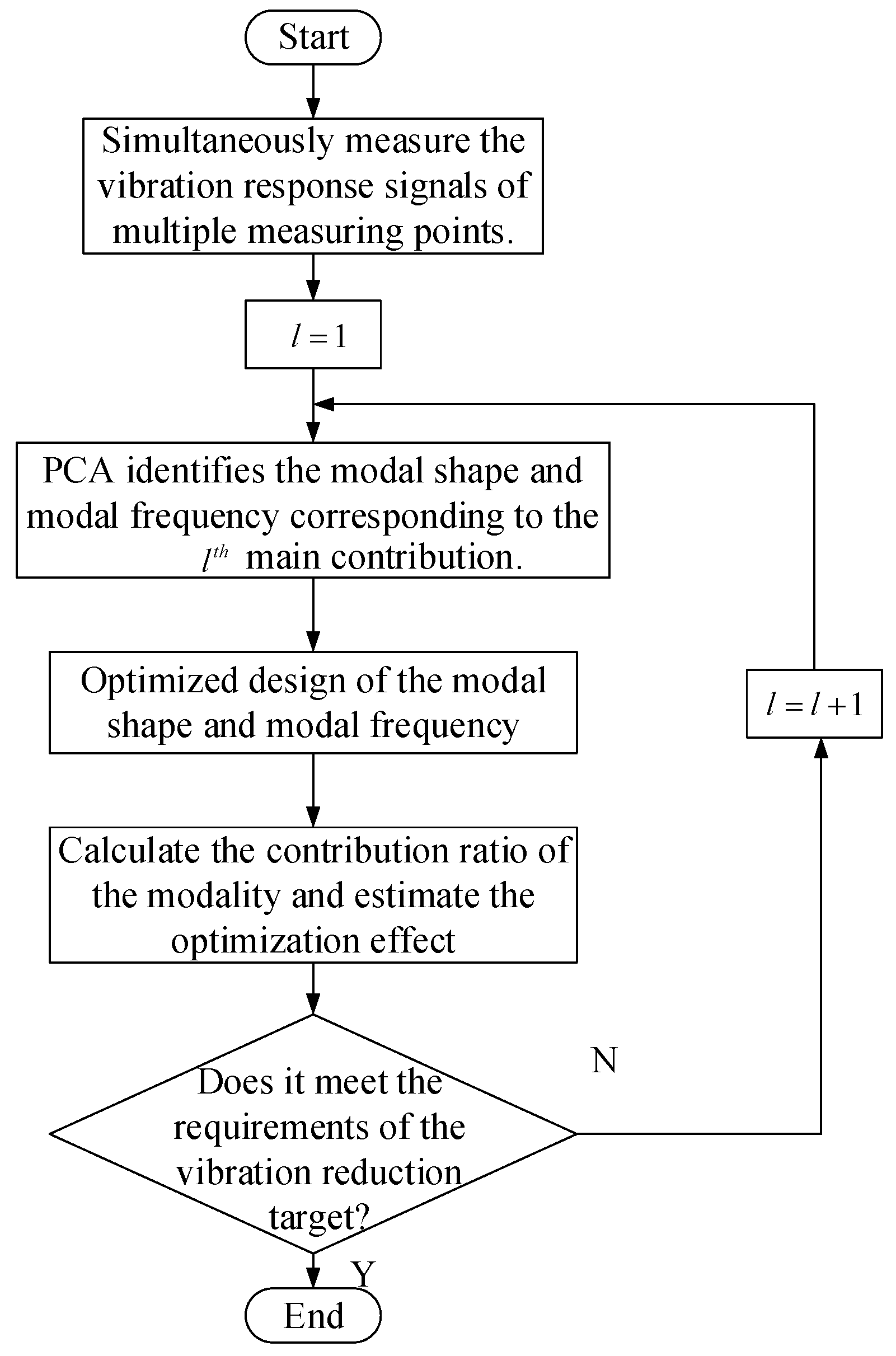
Figure 1. Active and passive control of vibration response based on PCA.
Applsci 10 00048 g001
Figure 2. Weight reduction process for old data.
Applsci 10 00048 g002
Figure 3. Procedure of PCAWF-based OMA for LTV structures.
Applsci 10 00048 g003
Figure 4. Procedure of ARPCAWF-based OMA for LTV structures.
Applsci 10 00048 g004
Figure 5. Procedure of ERPCAWF-based OMA for LTV structures.
Applsci 10 00048 g005
Figure 6. Three-DOF system model with external excitation.
Applsci 10 00048 g006
Figure 7. Identified mode shape MAC value of ERPCAWF-based OMA for different forgetting factors.
Applsci 10 00048 g007
Figure 8. Comparison of modal frequencies identified by ARPCAWF-, ERPCAWF-, ARPCA-, and ERPCA-based OMA and theoretical values.
Applsci 10 00048 g008
Figure 9. Relative errors between theoretical natural frequency and identified natural frequency by different methods.
Applsci 10 00048 g009
Figure 10. Comparison of MAC identified by different methods.
Applsci 10 00048 g010
Figure 11. Cumulative variance contribution rate of PCs extracted by ERPCAWF-based OMA at different moments when μ = 0.9990 : (a) 112.775 s; (b) 581.4 s; (c) 1275.3 s; and (d) 1987.2 s.
Applsci 10 00048 g011
Figure 12. Cumulative variance contribution rate of PCs extracted by ARPCAWF-based OMA at different moments when μ = 0.9990 : (a) 112.775 s; (b) 581.4 s; (c) 1275.3 s; and (d) 1987.2 s.
Applsci 10 00048 g012
Table 1. Performance comparison of multiple methods.
Algorithm-Based
OMA
Time ComplexitySpace ComplexityModal
Exchange
Number of Matrix
Decomposition
Accuracy ComparisonApplicable
Structure
P C A W F o ( N 3 ) o ( N 3 ) ExistTMeet the demandSLTV and FLTV
A R P C A W F o ( N 2 ) o ( N 2 ) ExistTSimilar as PCAWFSLTV and FLTV
E R P C A W F o ( N ) o ( N ) Avoid1BestSLTV and FLTV
L M P C A o ( N L ) , N < < L o ( N L ) , N < < L Exist T L + 1 Meet the demandSLTV
L M R P C A o ( N 2 ) o ( N 2 ) Exist T L + 1 Similar as LMPCASLTV
M W S I P C E o ( r M L ) , M < < N o ( N L ) , N < < L Exist0Better than LMPCASLTV
Table 2. MAC value of identified modal shape in ARPCAWF-, ERPCAWF-, ARPCA-, and ERPCA-based OMA when μ = 0.9990 .
OrderFirst OrderSecond OrderThird Order
ARPCAWF/ERPCAWF MAC value (112.775 s)0.8481/0.99980.8410/0.99960.9806/0.9998
ARPCA/ERPCA MAC value (112.775 s)0.8481/0.99980.8410/0.99960.9806/0.9998
ARPCAWF/ERPCAWF MAC value (581.4 s)0.9145/0.99960.8170/0.99570.8579/0.9961
ARPCA/ERPCA MAC value (581.4 s)0.9306/0.99990.8503/0.99460.9162/0.9947
ARPCAWF/ERPCAWF MAC value (1275.3 s)0.9151/1.00000.7696/0.61800.7626/0.6198
ARPCA/ERPCA MAC value (1275.3 s)0.9367/0.99990.6044/0.89940.6521/0.8984
ARPCAWF/ERPCAWF MAC value (1987.2 s)0.9183/0.99990.8368/0.85820.8232/0.8603
ARPCA/ERPCA MAC value (1987.2 s)0.9302/0.99990.5617/0.63810.5744/0.6352
Table 3. Time and space requirements of different methods.
MethodTime SpentSpace Requirement
ARPCAWF-based OMA23.141316 s41.1 MB
ERPCAWF-based OMA17.958531 s32.6 MB
ARPCA-based OMA23.168523 s41.2 MB
ERPCA-based OMA18.134408 s33.6 MB