Article

A Novel Optimization Layout Method for Clamps in a Pipeline System

1
School of Electromechanical and Automotive Engineering, Yantai University, Yantai 264005, China
2
School of Mechanical Engineering, Dalian University of Technology, Dalian 116024, China
*
Author to whom correspondence should be addressed.
Appl. Sci. 2020, 10(1), 390; https://doi.org/10.3390/app10010390
Submission received: 27 November 2019 / Revised: 24 December 2019 / Accepted: 2 January 2020 / Published: 4 January 2020
(This article belongs to the Section Acoustics and Vibrations)

Abstract

:
This paper proposes a novel optimization layout method for supporting clamps in a pipeline system. In this method, the global sensitivity analysis based on the Sobol method is presented to determine the influence of clamp position on the first-order frequency difference, the maximum vibration response displacement, and the maximum vibration stress. The modeling density of the finite element calculation is determined, and then a surrogate model of the relationship between the optimized input and the output is established through the neural network. The optimized position and orientation of the clamp are obtained by the genetic algorithm. Finally, a typical pipeline with clamps are conducted as an example to verify the effectiveness of the proposed optimization method. The simulations were compared with the experiment, and the result shows that the proposed optimization method can reduce the vibration of the pipeline system significantly, thus providing a new method for the arrangement of clamps in pipeline system.

1. Introduction

The aviation hydraulic pipeline system is connected to the hydraulic pump and other components to provide power for the elevator, rudder, undercarriage and other parts of the aircraft, and thus plays an important role on aircraft safety. Because of the lightweight requirements of the system, a large number of flexible clamps are used in the aviation hydraulic pipeline system, in which the support is weak, leading to serious coupling vibration and complicated vibration problems. When the frequency of external vibration is close to natural frequency of the pipeline system, structural resonance occurs, which might cause failures of the hydraulic pipeline system. Therefore, the investigation of the pipeline system vibration and its control has great value in engineering application.
Scholars have verified the effectiveness of various methods on the vibration control from the theoretical and experimental aspects [1,2,3,4,5,6]. According to mechanisms, these methods can be classified as follows:
  • Active control of the pipe directly to reduce the vibration;
  • Use damping materials between the hydraulic pipeline and the foundation to suppress the vibration transmission;
  • Control the fluid pulsation in the pipeline to reduce the vibration of the excitation source;
  • Adjust the number, position and layout of the supports in the system to change the dynamic characteristics of the system.
The implementation of active control requires space and energy input, making it more difficult to be applied in aero hydraulic pipeline systems. Due to the extremely small space and the complicated layout of pipes on aircraft, it is often unrealistic to set up a large damping device. In addition, due to the large temperature fluctuation of aero hydraulic pipeline system, the service life of the damping material is greatly limited. Pulsation attenuators tend to increase the mass of the system and can only reduce the vibration caused by fluid. This means that the first three methods have their limitations in aero applications. By adjusting the number and layout of pipeline supports, changing the dynamic characteristics of the system to reduce the vibration is at present the most commonly used, most convenient, and most economical method.
For many years, the arrangement of the clamps in the aero hydraulic pipeline systems was determined empirically according to the prototype. The number, position, and orientation of the clamps were mainly depended on the on-site experience of workers, while standards and norms are lack. Reasonable layout parameters can improve the dynamic characteristics of the pipeline system, avoiding the resonance, reducing the vibration amplitude and ensuring the reliable operation of the hydraulic system, which is of great significance to the safety of aircrafts [7]. Therefore, it is necessary to optimize the clamp layout by systematic and standardized methods to ensure the safe operation of the system.
Genetic algorithm (GA) is a kind of randomized search method that learns from evolution of biology. It was first proposed by Professor J. Holland in the United States in 1975 [8]. With inherent implicit parallelism and global optimization ability, the genetic algorithm has been applied in many fields [9,10,11,12,13] and showed good convergence. Among them, some scholars [9] combined BP (back-propagation) neural network [14] with GA. The neural network is relatively studied in theory and performance. Scholars [15,16,17,18] used neural network to make prediction and some of them [17,18] then input the predicted data into different algorithms to get optimal results. These works showed the strong nonlinear mapping capability, high efficiency, and flexible structure of neural network.
Focusing on the multi-support, long-span characteristics of the aviation hydraulic pipeline system, a typical clamp-supported Z-tube system was selected as the object. First, the sensitivity analysis method [19,20,21,22] was used to analyze the influence of the clamps position on the output. Based on the analysis results, the number of sampling points for each parameter in the finite element analysis was determined. Then, the neural network was used to build a surrogate model [23,24,25]. The validity of the modeling method was evaluated by comparing the predicted output with the actual output. Finally, based on the surrogate model, the position and direction of the clamp in the pipeline system were optimized.

2. Materials and Methods

2.1. Process of the Optimization

Because of the multi-support and long-span characteristics of the pipeline, the increase in the number of clamps means that the amount of calculation increases exponentially. This study, based on the neural network, proposed a surrogate model for optimizing the layout of the clamps, in which the nonlinear optimization of the genetic algorithm could be used to find the optimal solution for the model. First, the density of the finite element calculation was determined through the sensitivity analysis. Neural network was used to build relationships between the position of clamps, input and output data. The finite element analysis result was used to train the neural network to improve its accuracy. Finally, based on the output data, the optimal solution was found. The flow chart of the optimization is shown in Figure 1.

2.1.1. Global Sensitivity Analysis Based on Sobol Method

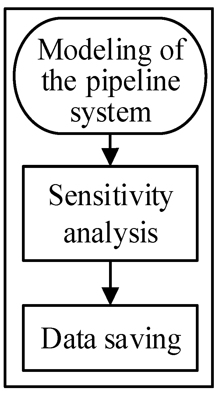
Sensitivity analysis is used to study the influence of each layout parameter on the output, which provides a guide for the system design. Currently, the most commonly used method of global sensitivity analysis is the Sobol method [22]. The flow chart of global sensitivity analysis is shown in Figure 2.
This method is based on the variance-based Monte Carlo method that defines a k-dimensional unit body as the spatial domain of the input parameters, which expressed as:
Ω k = { x | 0 x i 1 ; i = 1 , 2 , , k }
The main idea of the Sobol method is to decompose the function into the sum of the subitems.
f ( x 1 , x 2 , , x k ) = f 0 + i = 1 k f i ( x i ) + 1 i < j k f i j ( x i , x j ) + + f 1 , 2 , , k ( x 1 , x 2 , , x k ) ,
The function is decomposed to 2k subitems. Sobol uses a decomposition method based on multiple integrals. The total variance of the output f(x) is:
D = Ω k f 2 ( x ) d x f 0 2 .
The variance of each sub-item in Equation (2) is called the partial variance of each order, that is, s-order partial variance.
D i 1 , i 2 , i s = 0 1 0 1 f i 1 , i 2 , i s 2 ( x i 1 , x i 2 , x i s ) d x i 1 , d x i 2 , d x i s ( 1 i 1 < i s k ) .
Integrate Equation (2) over the entire range, and the relationship between the total variance and the partial variance of each order can be obtained in Equation (5):
D = I = 1 K D i + 1 i < j k D i j + + D 1 , 2 , k .
Define the sensitivity of each order as the ratio of the each-order partial variance to the total variance. The sensitivity of the S order, S i 1 , i 2 , i s , could be defined as:
S i 1 , i 2 , i s = D i 1 , i 2 , i s D ( 1 i 1 < < i s k ) .
When calculating the sensitivity of the input parameters, the normalization algorithm is used to normalize the position of the clamps. Sobol sampling is used to obtain the sampling points that need to be calculated, and the corresponding output is obtained by finite element analysis. The computational analysis could obtain global sensitivity coefficients for different parameters.

2.1.2. Prediction by Neural Network

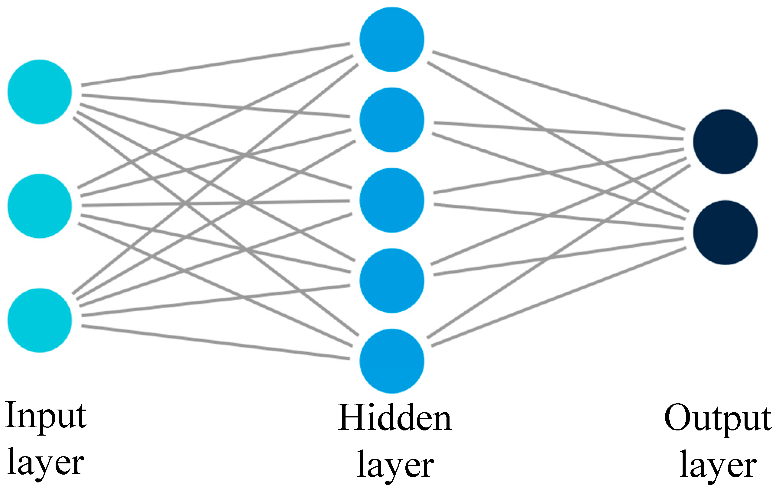
The flow chart of prediction by neural network is shown in Figure 3. Neural network usually consists of an input layer, a hidden layer, and an output layer. Each layer is distributed with a different number of nodes, and the nodes between the layers are connected. The transfer of data between neural networks is similar to the transmission of information in human neuronal structures. By training the neural network with data, the relationship between input and output can be obtained. The neural network topology is shown in Figure 4.
The main steps of establishing a surrogate model for optimizing the pipeline system using a neural network are as follows:
(1) Initialization of neural network
(2) Randomly select the input and output samples to calculate the input and output of neurons in each layer.
(3) Calculate the back-propagation error of each layer by comparing the network expectation and the actual output.
(4) According to the calculation result, the weight is corrected on the basis of the correction formula.
(5) Calculate the global error. If the error satisfies the preset accuracy requirement or the number of learning reaches the maximum convergence number, the correction is ended. Otherwise, the process will return to Step (3) and continue the loop until the convergence condition is met and a qualified neural network model is obtained.
According to Kolmogorov’s theory [26], a three-layer neural network with a hidden layer can simulate any nonlinear continuous function with precision. This makes the back-propagation neural network superior in nonlinear mapping ability, self-learning and self-adaptive to other algorithms. So, in this study, the neural network was used to construct the surrogate model.

2.1.3. Optimization by Genetic Algorithm

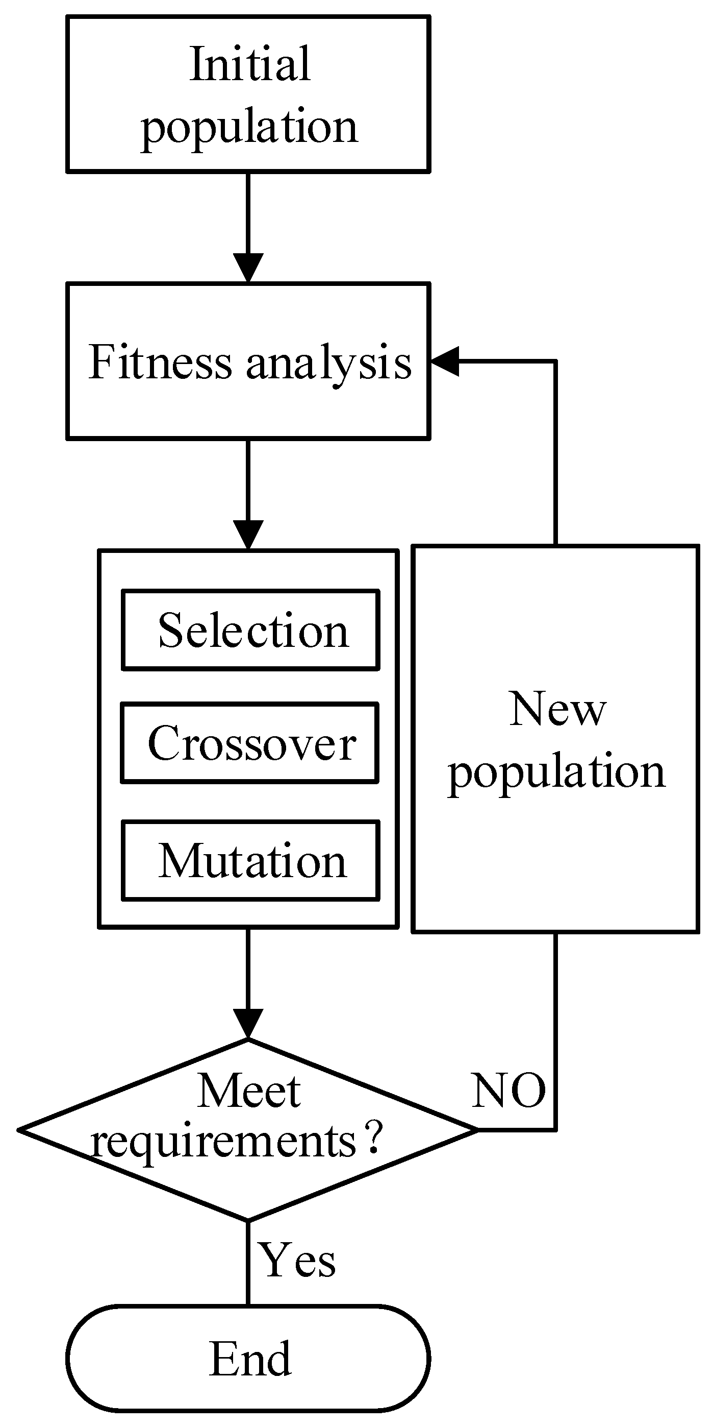
The flow chart of genetic algorithm is shown in Figure 5. Genetic algorithm is based on the natural selection to simulate the evolution process. The main steps of optimizing the clamp layout of the pipeline system using the genetic algorithm are as follows:
  • Set the population size and initialize all involved variables;
  • Select the initial group S according to the group isolation;
  • Calculate the fitness of the population, searching for individuals with higher fitness;
  • Selection, crossover, and mutation in the group and generate a transitional group ST;
  • Replace the individuals with lower fitness in S by the one with higher fitness in ST to generate a new group SN;
  • Check if the condition is met; if so, the loop is ended, and the individual with optimal fitness is outputted as the optimal solution; Otherwise, the process will return to Step 3 and continue until the termination condition is met.
The genetic algorithm has basically no restrictions on the target function, and thus has strong applicability. Multi-point parallel operation can effectively prevent the searching process from falling into the local optimal solution. Through large-scale parallel computing, efficiency can be significantly improved. Due to its strong applicability and reliability, the genetic algorithm has been widely used in various engineering fields in recent years. This study will use the genetic algorithm to optimize the model.

2.2. Optimization Function

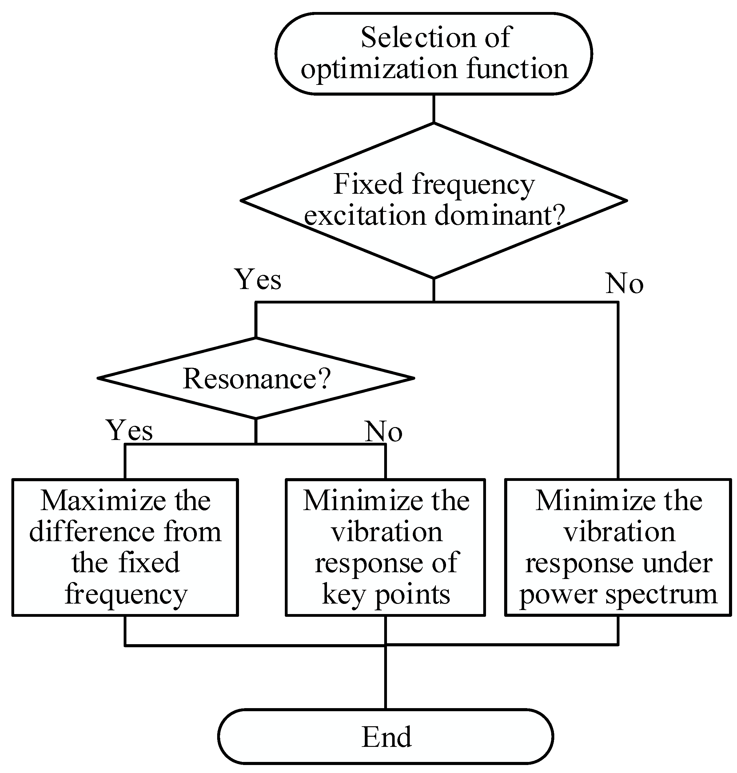
For pipeline system with harmonic excitation condition, in order to avoid resonance under external excitation, the pipeline system is required to work outside the resonance frequency range (generally outside its natural frequency of 20%). This requires the maximization difference between natural frequency of the pipeline system and excitation frequency. Sometimes, the vibration amplitudes at some critical locations are equally important when there is no resonance. Under such circumstances, minimizing the vibration amplitude of the critical locations can be the optimization goal to ensure that the vibration of the pipeline system is in the safe range. For the case when the range of excitation frequency with large range of variation or the working condition of the pipeline system during the whole life cycle is vital, the displacement or stress under the random load spectrum should be optimized to ensure the minimum vibration of the pipeline system. The selection of optimization function is shown in Figure 6.

2.3. Optimization Parameters

There is standard for parameters of the pipe material (0Cr18Ni9) and the HB3-25LB12B clamps are standard parts. Their strength can meet the requirements and the material parameters and structural parameters are unable to adjust. Therefore, in this paper, only the position and direction of the clamps are optimized.

2.4. Constraints

There are three ways to implement the constraints: limiting the search space method, feasible solution transformation method and penalty method. The distance requirements of the inputs are easy to implement, and the range of clamp positions can be specified using the limiting the search space method and. However, the mutual constraints between different inputs cannot directly implement and need to be taken into consideration. The penalty method is used to implement the constraints.
F ( x ) = { F ( x ) , Meet   all   constraints 0 , Any   one   of   the   constraints   is   not   met .
The optimization of genetic algorithm is aimed at maximizing fitness, and the fitness function is constructed by penalty function. The principle is shown in Equation (7). If the constraint requirement is met, F ( x ) takes the same value. If the constraint requirement is not met, F ( x ) is zero then. Based on this, the optimized pipeline system can be guaranteed to obtain the optimal solution under all constraints.

3. Results and Discussion

Aiming at a Z-shaped pipe, the optimization of clamps layout was carried out. The simulation results were compared with the experiment to verify the effectiveness of the method. This method can be then applied to more complicated pipeline systems.
The Z-shaped tube is shown in Figure 7. With L1, L2, L3 as input variables, first-order frequency difference, the displacement and stress of the system under random load are taken as outputs respectively. L1 and L3 range between 40–160 mm, while L2 ranges between 50–150 mm. The acceleration measure point is 200 mm from the left end. The random spectrum shown in Figure 8 was used as a load in the X direction of the piping system.

3.1. Sensitivity Analysis of the Input Variables

The sampling point is determined by Sobol sampling, and the sensitivity of the input variables L1, L2, L3 to the system first-order frequency, the displacement response of the random load, and the stress response are analyzed using the Sobol method. The obtained sensitivity bar chart is shown in Figure 9.
As can be seen from Figure 9, changing the value of L1 and L3 will significantly influence the first-order frequency and the stress of the pipeline system under random excitation. The value of L2 has a larger influence on the displacement. The different influence of different input parameters on the output parameters should be taken into consideration. In this paper, L1 and L3 are equally divided into six parts, and L2 is divided into four equal parts. It is necessary to calculate 6 × 4 × 6 = 144 points. Through finite element analysis, the relationship between input and output under different combinations is obtained.

3.2. Prediction by Neural Network

The neural network is used to build a surrogate model between inputs and outputs. In this paper, the neural network is used to implement the multi-input and multi-output function. The number of hidden layers is set to two.
Neural networks rely on a variety of transfer functions to transfer data. There are a variety of transfer functions, of which commonly used are three: log-sigmoid, tan-sigmoid and purelin [27]. Tan-sigmoid was used as the transfer function for the input layer while purelin for the hidden layer of neural network due to their better fitness and the accuracy in prediction in this case.
There is no uniform standard for the choice of the number of hidden nodes. The general principle observed is to use a simple network structure and as few neuronal nodes as possible which meet the precision requirements and reflect the relationship of input and output. The learning rate is generally selected between 0.01 and 0.8. When the learning rate is low, the system stability is good, while training takes longer. Finite element calculation is the most time-consuming in the whole optimization process, and the optimization process is short compared to the modeling time. It is finally determined that the number of hidden nodes in the first layer is 10, the number of nodes in the secondary layer is 3, and the learning rate is set to 0.01.
Figure 10 shows the errors between predicted results and the results of finite element analysis. By comparing the predicted output with the 30 sets of simulation data, it can be obtained that errors are within 2%, which meets the requirements of the engineering. The errors of the first-order frequency are basically less than 0.5% and are obviously less than the errors of displacement and stress under the random load. The possible reason for this is that the finite element mesh division is not fine enough. The displacement and stress under random load are greatly influenced by the mesh, resulting in large fluctuations in input data. The accuracy of calculations can be improved by refining the meshes, however this can greatly increase the time for calculation. In engineering, the mesh size should be selected reasonably.

3.3. Optimization by Genetic Algorithm

In order to implement the generic algorithm, 6 main factors (parameter coding, initial population setting, fitness function design, control parameter setting and constraint setting) need to be taken into consideration.
Commonly used coding methods include binary coding and real-number encoding. The real-number encoding method is more suitable in this case and the efficiency is high. The selection of some important parameters (mainly include population n, mutation rate Pm, crossover rate Pc, and maximum number of iterations maxgen) directly affects the performance of the genetic algorithm. Currently there is no accepted method for determining the value of parameters in genetic algorithm. It is normally taken that n = 20~100, the mutation rate Pm = 0.0001~0.1, and the crossover rate Pc = 0.4~0.99. In this paper, the sets of data n = 50, the maximum number of iterations maxgen = 100, the crossover probability Pc = 0.7 and the mutation probability Pm = 0.05 are determined as parameters in genetic algorithm due to limited computing resources.
The implementation of constraints in this paper is by constructing the penalty function. The selection of the adaptability function directly affects the convergence speed and the accuracy of the optimal solution of the genetic algorithm. Genetic algorithms basically do not need other information in evolutionary search, except the adaptability function based on the search of individuals. Therefore, the design of the adaptability function should be simple, efficient, and distinguished.
There are two cases to optimize the clamp-pipeline system. One is to maximize the frequency difference and the other is to minimize the displacement or stress.
When maximizing the frequency difference, the fitness function should be:
F ( x ) = { f ( x ) C min , Meet   all   constraints 0 , Any   one   of   the   constraints   is   not   met .
where f(x) is the absolute value of the difference between the first-order frequency and the excitation frequency. Cmin is the minimum estimate value of f(x).
When minimizing the displacement or stress, the fitness function should be:
F ( x ) = { C max f ( x ) , Meet   all   constraints 0 , Any   one   of   the   constraints   is   not   met .
where f(x) is the displacement or stress under certain excitation. Cmax is the maximum estimate value of f(x). The results predicted by the neural network surrogate model shows that the possible maximum displacement is 6 × 10⁻⁵ m and the maximum stress value is 50 MPa.
The peak frequency of the vibration in a certain aircraft under working conditions consist of the frequency of the high and low-pressure rotors and their multiplications. The low-pressure rotor frequency is 159 Hz and the high-pressure rotor frequency is 206 Hz. The first-order frequency in the trial data is generally smaller than the low-pressure rotor frequency. When the first-order frequency difference is maximized, the value of the clamp position L1–L3 is shown in Figure 11. The frequency difference convergence curve is shown in Figure 12.
Figure 11 and Figure 12 shows that after serval iterations, L1, L2, L3 converge at 40.3 mm, 50.7 mm, 41.7 mm respectively. The maximum frequency difference converges at 68.41 Hz at the 47th generation. First-order frequency of the system is 90.59 Hz, which is basically the same as the result of simulation (89.98 Hz).
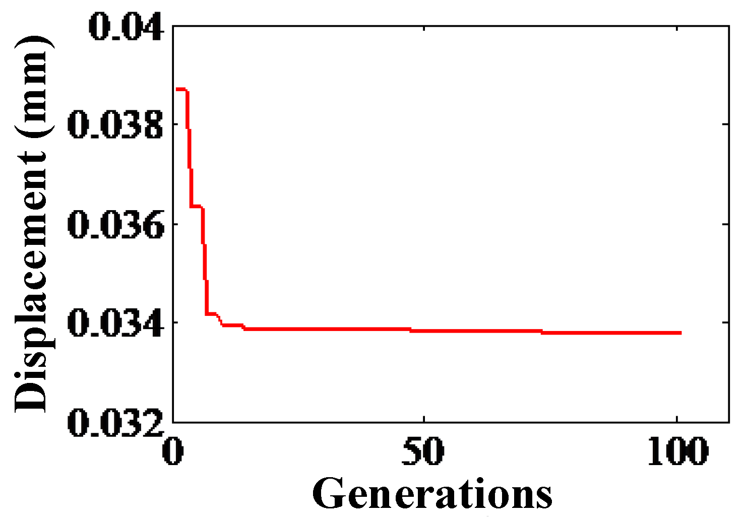
When minimizing the displacement under random loads, the extraction process of clamp positions (L1–L3) is shown in Figure 13, and the maximum displacement convergence curve is shown in Figure 14.
Figure 13 and Figure 14 shows that after serval iterations, L1, L2, L3 converge at 111.3 mm, 100.8 mm, 110.7 mm respectively. The maximum displacement converges at 0.0338 mm at 77th generation.
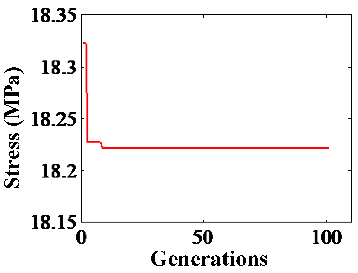
When minimizing the stress under random loads, the extraction process of clamp positions (L1–L3) is shown in Figure 15. The maximum stress convergence curve is shown in Figure 16.
Figure 15 and Figure 16 shows that after serval iterations, L1, L2, and L3 converge at 128.3 mm, 85.7 mm, 122.7 mm respectively. The maximum displacement converges at 18.22 MPa at 11th generation.
The parameters of the clamp position and the optimization results of the above optimization schemes are listed in Table 1.
As can be seen from Table 1, when maximizing the first-order frequency difference, the optimization makes the clamp adjacent distance maximum. At this time, the system’s first-order frequency is the smallest, and the first-order frequency difference before and after optimization is maximum. When minimizing the displacement, the displacement response and stress response are small, but the first-order frequency difference is small as well. When minimizing the stress, a large displacement is also caused.

3.4. Validation of the Optimization

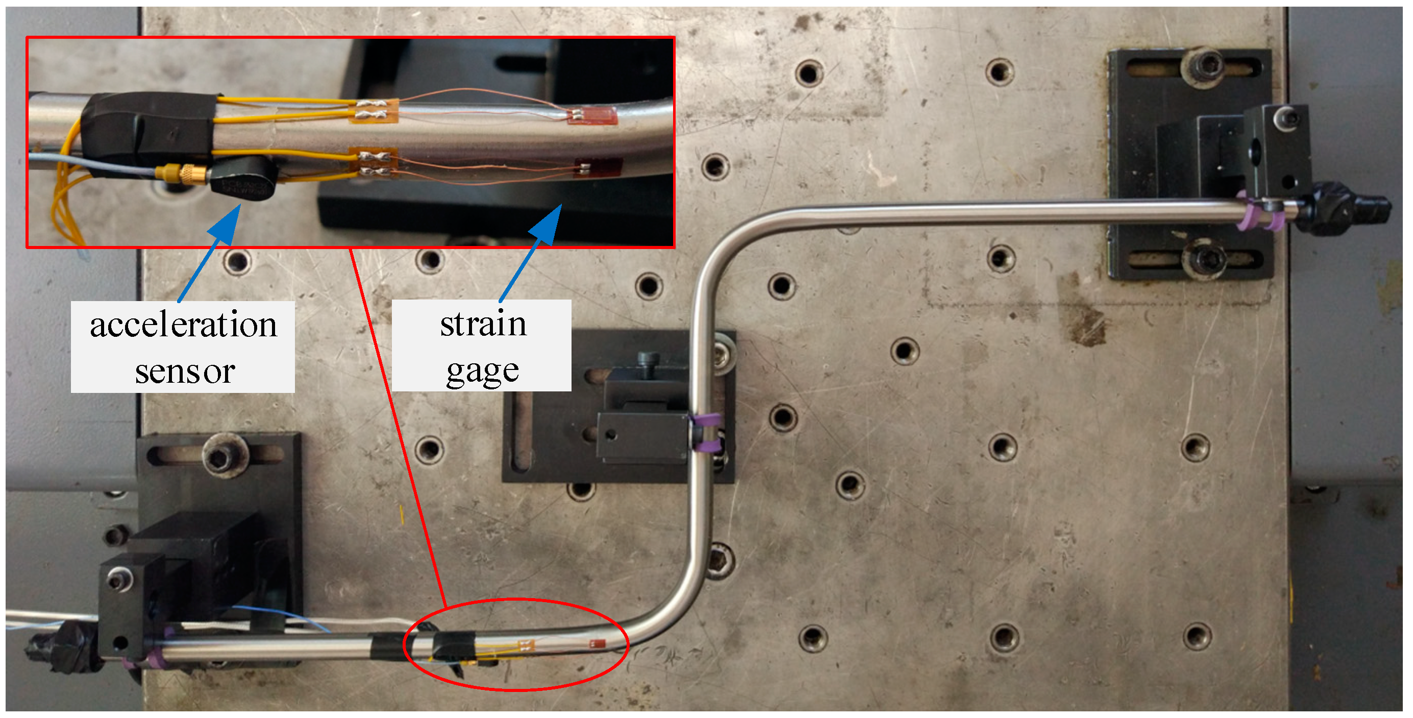
An experimental platform was set up to verify the optimization results. Due to the limitation of the experiment conditions, only two sets of optimization results with first-order frequency difference maximization and stress response minimization were verified, and the position of acceleration sensor was consistent with the simulation. Simulation results show that the maximum stress is in the clamp band, and it’s impossible to mount strain gauge there. In this experiment, strain gauges are mounted along the horizontal and vertical direction near the bend. The clamp-pipe system before optimization is shown in Figure 17.
Adjust the position of the clamps according to the values of L1, L2 and L3 in Table 1 respectively as shown in Figure 18, the first-order frequency and stress peak-peak value of the optimized pipeline system is obtained in Table 2.
As can be seen from Table 2, the first-order frequency difference before and after optimization increased from 49.4 Hz to 70.2 Hz, which is basically the same as the simulation results. The horizontal directional stress value at the bending point of the pipeline system is reduced from 9.82 MPa to 5.54 MPa, and the peak of the vibration stress response peak has a large degree of reduction, which means that it can significantly reduce the pressure of the pipe system by optimizing the clamp arrangement.

4. Conclusions and Prospects

In this paper, a complex pipeline model with multi-supports is established. A novel optimizing method for the design of the clamp layout is formed. Some new results are listed as follows:
(1) For the complex pipeline system with multi-clamps, the surrogate model of clamp position and vibration output is established by back-propagation algorithm. The accuracy of the neural network agent model is verified by random selection of clamp position within the optimization range. The results show that the prediction error of the first-order frequency of surrogate model is about 0.5%, and the prediction error of the random load displacement and stress is about 2%, which meets the engineering application.
(2) The genetic algorithm is proposed to optimize the position of clamps on a Z-shaped pipe under the surrogate model. Results show that optimization results have a large difference for different optimization goals. When maximizing frequency difference, the optimization result increases the first-order frequency difference by 42.11%; when minimizing vibration stress, the optimization result reduces the maximum vibration stress by 43.58%. In the engineering field, the specific optimization scheme should be determined on the basis of practical optimization goals. The proposed optimization method can provide a new method for the arrangement of clamps in pipeline system.
(3) In the experiment, the strain gauge is used to measure the stress at a fixed position (a small area). This position may be slightly different from the theoretical point of stress concentration where the stress varies greatly nearby. In addition, the position of the clamps in this case may not be as accurate as they were in the finite element model, and this would influence the position of the maximum stress point as well. Thus, the measured value is much smaller than the theoretical value.
(4) In most scientific research, the stress simulation of isotropic material is generally based on the von mises equivalent stress without consideration of specific directions. In this paper, we mainly focus on the effectiveness of this optimization method. So, in our simulation, only the magnitude of Von Mises equivalent stress was studied. Simulation under different directions could be taken into consideration in the future work.

Author Contributions

Conceptualization, P.G.; methodology, P.G.; software, P.G.; validation, J.L., J.Z. and Y.T.; formal analysis, J.L.; investigation, J.Z.; resources, Y.T.; data curation, J.L.; writing—original draft preparation, P.G.; writing—review and editing, J.L.; visualization, Y.T.; supervision, J.Z.; project administration, Q.H.; funding acquisition, P.G. All authors have read and agreed to the published version of the manuscript.

Funding

This research was funded by National Natural Science Foundation of China, grant number 51805462.

Conflicts of Interest

The authors declare no conflict of interest.

References

  1. Ray, M.C.; Reddy, J.N. Active damping of laminated cylindrical shells conveying fluid using 1–3 piezoelectric composites. Compos. Struct. 2013, 98, 261–271. [Google Scholar] [CrossRef]
  2. Herold, S.; Mayer, D. Adaptive Piezoelectric Absorber for Active Vibration Control. Actuators 2016, 5, 7. [Google Scholar] [CrossRef] [Green Version]
  3. Tan, J.; Ho, S.M.; Zhang, P.; Jiang, J. Experimental Study on Vibration Control of Suspended Piping System by Single-Sided Pounding Tuned Mass Damper. Appl. Sci. 2019, 9, 285. [Google Scholar] [CrossRef] [Green Version]
  4. Sorokin, S.; Holst-Jensen, O. On Power Flow Suppression in Straight Elastic Pipes by Use of Equally Spaced Eccentric Inertial Attachments. J. Vib. Acoust. 2012, 134, 041003. [Google Scholar] [CrossRef]
  5. Lu, X.; Zhang, L.; Cui, Y.; Li, Y.; Ye, L. Experimental and theoretical study on a novel dual-functional replaceable stiffening angle steel component. Soil Dyn. Earthq. Eng. 2018, 114, 378–391. [Google Scholar] [CrossRef]
  6. Ghayesh, M.H.; Farokhi, H.; Farajpour, A. Pulsatile vibrations of viscoelastic microtubes conveying fluid. Microsyst. Technol. 2019, 25, 3609. [Google Scholar] [CrossRef]
  7. Zhang, Y.; He, L.; Yang, J.; Wan, F.; Gao, J. Vibration Control of an Unbalanced Single-Side Cantilevered Rotor System with a Novel Integral Squeeze Film Bearing Damper. Appl. Sci. 2019, 9, 4371. [Google Scholar] [CrossRef] [Green Version]
  8. Holland, J.H. Adaptation in Natural and Artificial Systems; The University of Michigan Press: Ann Arbor, MI, USA, 1975. [Google Scholar]
  9. Yu, F.; Xu, X. A short-term load forecasting model of natural gas based on optimized genetic algorithm and improved BP neural network. Appl. Energy 2014, 134, 102–113. [Google Scholar] [CrossRef]
  10. Konak, A.; Coit, D.W.; Smith, A.E. Multi-objective optimization using genetic algorithms: A tutorial. Reliab. Eng. Syst. Saf. 2006, 91, 992–1007. [Google Scholar] [CrossRef]
  11. Zhihui, L.; Wang, M.Y.; Kedian, W.; Xuesong, M. Fixture performance Improv. by an accelerated integral method of fixture layout and clamping force plan. Proc. Inst. Mech. Eng. Part B J. Eng. Manuf. 2013, 227, 1819–1829. [Google Scholar] [CrossRef]
  12. Zhang, X.P.; Yang, W.Y.; Li, M. Fixture Layout and Clamping Force Optimization for Large-Scale Workpiece Using Augmented Lagrangian Method. Appl. Mech. Mater. 2010, 29–32, 560–565. [Google Scholar] [CrossRef]
  13. Chen, W.; Ni, L.; Xue, J. Deformation control through fixture layout design and clamping force optimization. Int. J. Adv. Manuf. Technol. 2008, 38, 860–867. [Google Scholar] [CrossRef]
  14. Rumelhart, D.E.; Mcclelland, J.L. Parallel Distributed Processing: Explorations in the Microstructure of Cognition: Foundations; MIT Press: Cambridge, MA, USA, 1986. [Google Scholar]
  15. Zheng, Y.; Zhong, H.; Fang, Y.; Zhang, W.; Liu, K.; Fang, J. Rockburst Prediction Model Based on Entropy Weight Integrated with Grey Relational BP Neural Network. Adv. Civ. Eng. 2019, 2019, 8. [Google Scholar] [CrossRef]
  16. Ren, C.; An, N.; Wang, J.; Li, L.; Hu, B.; Shang, D. Optimal parameters selection for BP neural network based on particle swarm optimization: A case study of wind speed forecasting. Knowl. Based Syst. 2014, 56, 226–239. [Google Scholar] [CrossRef]
  17. Wang, D.; Luo, H.; Grunder, O.; Lin, Y.; Guo, H. Multi-step ahead electricity price forecasting using a hybrid model based on two-layer decomposition technique and BP neural network optimized by firefly algorithm. Appl. Energy 2017, 190, 390–407. [Google Scholar] [CrossRef]
  18. Cui, K.; Qin, X. Virtual reality research of the dynamic characteristics of soft soil under metro vibration loads based on BP neural networks. Neural Comput. Appl. 2018, 29, 1233–1242. [Google Scholar] [CrossRef]
  19. Pronzato, L. Sensitivity analysis via Karhunen–Loève expansion of a random field model: Estimation of Sobol’ indices and experimental design. Reliab. Eng. Syst. Saf. 2019, 187, 93–109. [Google Scholar] [CrossRef] [Green Version]
  20. Roostaie, T.; Farsi, M.; Rahimpour, M.R. Dehydration of crude oil by cellulose-based demulsifiers: Statistical modeling sensitivity analysis and optimization. Pet. Sci. Technol. 2019, 37, 2134–2141. [Google Scholar] [CrossRef]
  21. Jaxa-Rozen, M.; Kwakkel, J. Tree-based ensemble methods for sensitivity analysis of environmental models: A performance comparison with Sobol and Morris techniques. Environ. Model. Softw. 2018, 107, 245–266. [Google Scholar] [CrossRef]
  22. Nossent, J.; Elsen, P.; Bauwens, W. Sobol’ sensitivity analysis of a complex environmental model. Environ. Model. Softw. 2011, 26, 1515–1525. [Google Scholar] [CrossRef]
  23. Tripathy, R.K.; Bilionis, I. Deep UQ: Learning deep neural network surrogate models for high dimensional uncertainty quantification. J. Comput. Phys. 2018, 375, 565–588. [Google Scholar] [CrossRef] [Green Version]
  24. Chen, X.; Zhou, H.; Li, Y. Effective design space exploration of gradient nanostructured materials using active learning based surrogate models. Mater. Des. 2019, 183, 108085. [Google Scholar] [CrossRef]
  25. Meng, D.; Yang, S.; Zhang, Y.; Zhu, S.P. Structural reliability analysis and uncertainties-based collaborative design and optimization of turbine blades using surrogate model. Fatigue Fract. Eng. Mater. 2019, 42, 1219–1227. [Google Scholar] [CrossRef]
  26. Hecht-Nielsen, R. Kolmogorov’s Mapping Neural Network Existence Theorem. In Proceedings of the International Conference on Neural Networks, San Diego, CA, USA, 21–24 June 1987; Volume 3, pp. 11–13. [Google Scholar]
  27. Ansari, H.R.; Zarei, M.J.; Sabbaghi, S.; Keshavarz, P. A new comprehensive model for relative viscosity of various nanofluids using feed-forward back-propagation MLP neural networks. Int. Commun. Heat Mass 2018, 91, 158–164. [Google Scholar] [CrossRef]
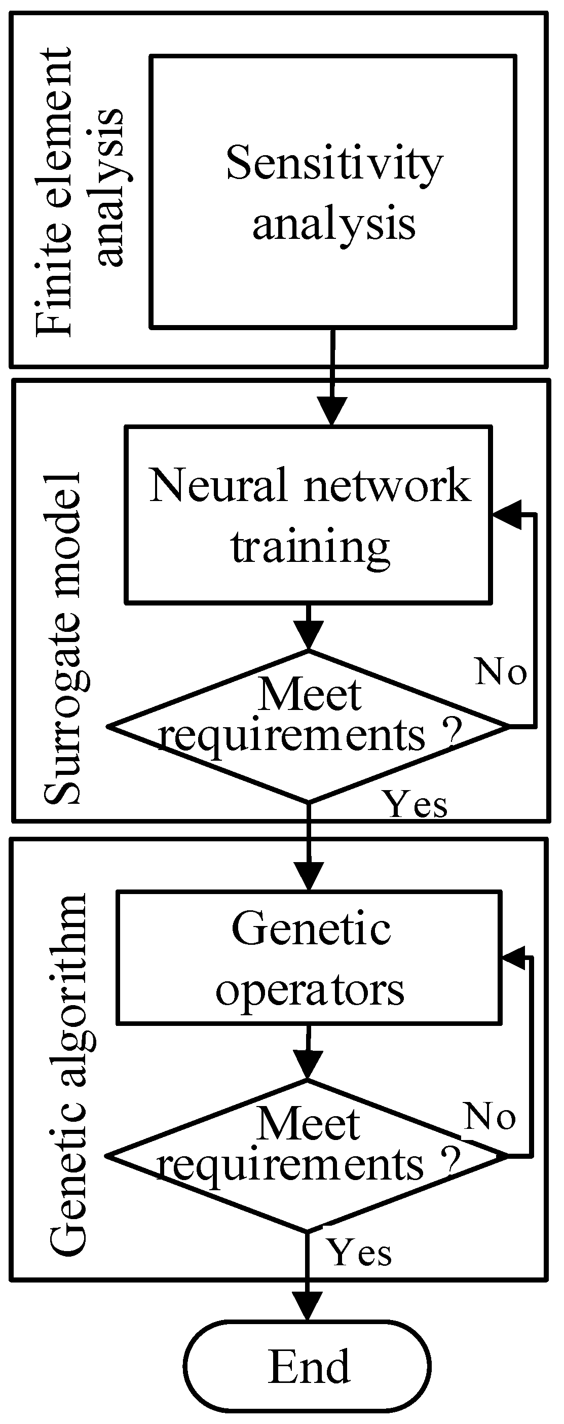
Figure 1. Flow chart of optimization algorithm.
Applsci 10 00390 g001
Figure 2. Flow chart of global sensitivity analysis.
Applsci 10 00390 g002
Figure 3. Flow chart of prediction by neural network.
Applsci 10 00390 g003
Figure 4. Topology diagram of neural network.
Applsci 10 00390 g004
Figure 5. Flow chart of genetic algorithm.
Applsci 10 00390 g005
Figure 6. Selection of optimization function.
Applsci 10 00390 g006
Figure 7. Position of the clamp.
Applsci 10 00390 g007
Figure 8. Power spectral density curve.
Applsci 10 00390 g008
Figure 9. Sensitivity histogram about input variables to output parameters: (a) Parameters sensitivity to first-order frequency; (b) Parameters sensitivity to displacement; (c) Parameters sensitivity to stress.
Applsci 10 00390 g009
Figure 10. Errors of neural network prediction.
Applsci 10 00390 g010
Figure 11. Selection of input variables: (a) Selection of L1; (b) Selection of L2; (c) Selection of L3.
Applsci 10 00390 g011
Figure 12. Convergence curve of frequency difference.
Applsci 10 00390 g012
Figure 13. Selection of input variables: (a) Selection of L1; (b) Selection of L2; (c) Selection of L3.
Applsci 10 00390 g013
Figure 14. Convergence curve of displacement.
Applsci 10 00390 g014
Figure 15. Selection of input variables: (a) Selection of L1; (b) Selection of L2; (c) Selection of L3.
Applsci 10 00390 g015
Figure 16. Convergence curve of stress.
Applsci 10 00390 g016
Figure 17. Clamp-pipe system before optimization.
Applsci 10 00390 g017
Figure 18. Clamp-pipe system after optimization: (a) Maximizing frequency difference; (b) Minimizing the stress.
Applsci 10 00390 g018
Table 1. Clamps layout before and after optimization.
Optimization GoalL1 (mm)L2 (mm)L3 (mm)Frequency Difference (Hz)Displacement (mm)Stress (MPa)
Before Optimization501005050.420.050229.56
Maximizing the frequency difference40.350.741.768.410.037437.54
Minimizing the displacement111.3100.8110.737.540.033820.75
Minimizing the stress128.385.7122.737.240.084918.22
Table 2. Vibration Characteristics of clamp-pipe system before and after optimization.
CharacteristicsMethodsDirectionbefore Optimizationafter Optimization
Frequency (Hz)Experiment/48.470.2
Simulation/50.4268.41
Stress (MPa)ExperimentHorizontal9.825.54
Vertical6.464.13
Simulation/29.5618.022