Prediction of Radiation Frost Using Support Vector Machines Based on Micrometeorological Data

Abstract

Radiation frost happens frequently in the Yangtze River Delta region, which causes high economic loss in agriculture industry. It occurs because of heat losses from the atmosphere, plant and soil in the form of radiant energy, which is strongly associated with the micrometeorological characteristics. Multidimensional and nonlinear micrometeorological data enhances the difficulty in predicting the radiation frost. Support vector machines (SVMs), a type of algorithms, can be supervised learning which widely be employed for classification or regression problems in research of precision agriculture. This paper is the first attempt of using SVMs to build prediction models for radiation frost. Thirty-two kinds of micrometeorological parameters, such as daily mean temperature at six heights (T_mean0.5, T_mean1.5, T_mean2.0, T_mean3.0, T_mean4.5 and T_mean6.0), daily maximum and minimum temperatures at six heights (T_max0.5, T_max1.5, T_max2.0, T_max3.0, T_max4.5 and T_max6.0, and T_min0.5, T_min1.5, T_min2.0, T_min3.0, T_min4.5 and T_min6.0), daily mean relative humidity at six heights (RH_0.5, RH_1.5, RH_2.0, RH_3.0, RH_4.5 and RH_6.0), net radiation (R_n), downward short-wave radiation (R_sd), downward long-wave radiation (R_ld), upward long-wave radiation (R_lu), upward short-wave radiation (R_su), soil temperature (T_soil) and soil heat flux (G) and daily average wind speed (u) were collected from November 2016 to July 2018. Six combinations inputs were used as the basis dataset for testing and training. Three types of kernel functions, such as linear kernel, radial basis function kernel and polynomial kernel function were used to develop the SVMs models. Five-fold cross validation was conducted for model fitting on training dataset to alleviate over-fitting and make prediction results more reliable. The results showed that an SVM with the radial basis function kernel (SVM-BRF) model with all the 32 micrometeorological data obtained high prediction accuracy in training and testing sets. When the single type of data (temperature, humidity and radiation data) was used for the SVM without any functions, prediction accuracy was better than that with functions. The SVM-BRF model had the best prediction accuracy when using the multidimensional and nonlinear micrometeorological data. Considering the complexity level of the model and the accuracy of prediction, micrometeorological data at the canopy height with the SVM-BRF model has been recommended for radiation frost prediction in Yangtze River Delta and probably could be applied in elsewhere with the similar terrains and micro-climates.

1. Introduction

Radiation frosts happen frequently in the middle and lower reaches of the Yangtze River, China, leading to huge losses of famous tea production [1,2]. Generally, radiation frost occurs at the specific meteorological characteristics with a clear and calm sky, and a high relative humidity. During a typical frost night, heat in the form radiant energy, is easily lost from the underlying surface to the sky. Under a clear night-time sky, there is much more heat radiated out from the surface than received which results in the decrease of air temperature [3,4]. A temperature inversion will form when the air temperature falls faster near the radiant surface. The sensible heat from the soil and air near the radiant surface is reduced, which causes a net loss of energy from surface. Based on the energy balance in the plant-soil-atmosphere system, sensible heat flux downwards from the air and upwards from the surface soil to replace the heat losses. Dew point temperature is the temperature at which water vapor condenses into liquid water [5]. Generally, relative humidity is a relative measurement of how humid the air is, the dewpoint temperature is an absolute measurement of how much water is in the air. When warm air contracts with a cooler surface, water vapor will condense. With the further decrease of air temperature to frost point, the water vapor will be frozen [4,6]. A light frost event will happen when the nighttime temperature is below 0 °C. A heavy frost occurs after a period of more than four consecutive hours of air temperature that is below −4 °C [4].

Several methods have been attempted to predict frost events in recent decades, but many involve the empirical relationship to the dewpoint temperature (T_d). Saenko pointed that frost may happen when the T_d is less than 6 °C, and more likely to happen as it is below 0 °C in Victoria [7]. In Canada the nocturnal minimum temperature is deduced as equal to (T_max + T_d)/2 minus a correction parameter related to the wind speed and cloudiness. T_max is the highest temperature in the previous day (FAO). However, radiation frost is caused by kinds of specific and complicated meteorological conditions. Simply using the dew temperature to present the radiation frost has certain limitation and inaccuracy. Generally, frost warning systems and models are developed using meteorological variables, such as maximum and minimum temperatures, dewpoint temperature, cloud cover, precipitation and average wind speed [8,9,10]. Hu et al. [11] statistically analyzed the historical data of late frost occurrence in Zhenjiang of China between March and April from 1979 to 2008 and established the prediction models based on the seasonal disasters grey method. The results found that grey prediction model had the excellent accuracy with the ratio between posteriori errors less than 0.35 and the model accuracy above 0.95. However, the model was limited to be used for predicting the first and last frost occurrence dates. Lee et al. [12] attempted using logistic regression (LR) and decision tree (DT) techniques to develop the prediction models for spring frosts in Korea. The average values of hit rate and probability of detection were all high in both of LR and DT. However, only eight limited meteorological variables, such as the minimum temperature, difference between maximum and minimum temperature, grass minimum temperature, dewpoint temperature, cloud cover, mean relative humidity, minimum relative humidity and wind speed, were used as variables for the prediction models. It was not accurate because those models ignored the radiation meteorological data. The energy budget balance is closely associated with the radiation in a typical radiation frost night. Radiated energy is the main form of the energy absorbed and lost in the eco-system. LR and DT techniques indeed had a good predict accuracy with simply and linearly data. However, the formation of radiation frost is closely related to the complex micrometeorological data, especially the microclimate around the canopy. Meanwhile, multidimensional and nonlinear microgeological data increase the difficulty of radiation frost prediction.

The support vector machines (SVMs) are originally developed for pattern recognition. It is a new general learning method based on the statistical theory of solving the quadratic optimization problem and seeking the global optimal solution [13]. SVMs are the algorithms that can be supervised learning, which mainly are employed for classification or regression problems. Kernel trick technique is used to transform the data. Based on these transformations, an optimal boundary is found out between these possible outputs [14]. Generally, micrometeorological data in a frost night are multidimensional and nonlinear, which increase the difficulty in prediction. In recent years, it has been applied in solving the issues of classification, function approximation and prediction related to precision agriculture, agricultural water management and bio-meteorology [14,15,16,17,18,19]. Its successfully application in precision agriculture makes frost prediction reliable.

While, the SVMs employed in frost prediction have not been completely attempted yet. This paper is the first attempt to evaluate the possibility of using the SVMs to predict the radiation frost in the Yangtze River region. Therefore, the objective of this study is using SVMs to develop the prediction models with different input combinations of meteorological data. The specific tasks are (1) to determine the effects of various input combinations of meteorological data for radiation frost prediction, (2) to develop the SVMs models based on three kinds kernel functions (linear function, radial basis function and polynomial function) for frost protection using the properly meteorological data and (3) to compare the prediction accuracy of four SVMs models and determine the optimal model and most related micrometeorological parameters in predicting the radiation frost.

2. Materials and Methods

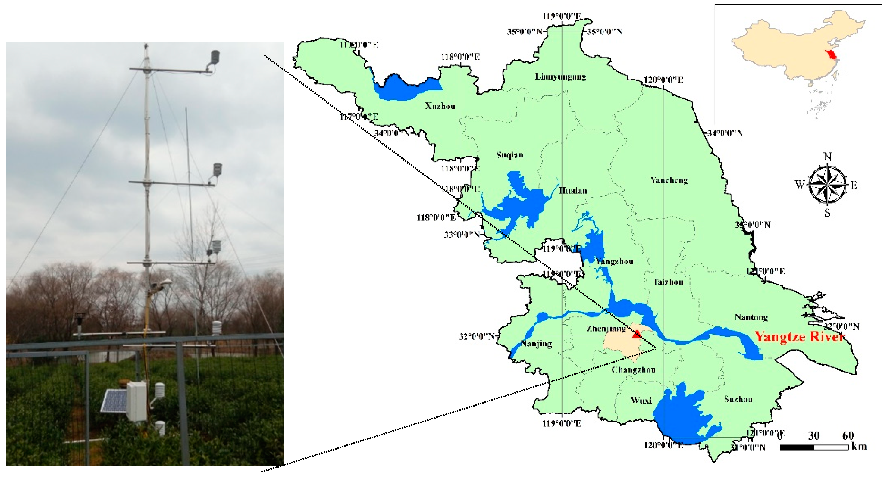
2.1. Experimental Site

The experimental site was located at Danyang Maichun Tea Farm, a common tea farm in the Middle-Lower Yangtze River region of east China (Figure 1). It is a typical hilly topography with the average altitude of 18.5 m. The mean annual precipitation is 1029.1 mm and the annual mean temperature is 15.5 °C, which belongs to the typical moderate sub-tropical climate. Radiation frosts frequently happened in the late autumn, winter and early spring [1,2].

2.2. Micro-Meteorological Data Collection and Analysis

Thirty-one types of micrometeorological data were collected by the scientific weather station (Figure 1). Net radiation (R_n), downward short-wave radiation (R_sd), downward long-wave radiation (R_ld), upward long-wave radiation (R_lu) and upward short-wave radiation (R_su) was measured by a four component radiometer (CNR4, Kipp and Zonen, Delft, Netherlands) at the height of 2.5 m. Air temperature and humidity at the height of 0.5 m, 1.0 m, 1.5 m, 3.0 m, 4.0 m and 6.0 m were measured with six HC2S3 (Campbell Scientific, Logan, UT, USA), respectively. Soil temperature (T_soil) was measured by Hydra Probe II at the depth of 5.0 cm (Stevens, Portland, OR, USA). Soil heat flux (G) was measured by HFP01SC (Hukseflux, Delft, Netherlands). Wind speed (u) was measured by 2-D sonic wind sensor (Wind Sonic C1-L, Campbell Scientific, Logan, UT, USA) at the height of 2.5 m. Soil heat flux plates was placed at the depth of 5 cm. All sensors have been calibrated before carrying out the experiment. CR3000 data loggers (Campbell Scientific, Logan, UT, USA) were used to collect the meteorological data and the data sampling frequency of all the sensors is 0.5 Hz. The collection interval of all the sensors was 10 min. Continuous and long-time series meteorological data were collected from 10 November 2016 to 19 July 2018. They were micro-daily maximum/minimum air temperature at five heights (T_mean0.5, T_mean1.5, T_mean2.0, T_mean3.0, T_mean4.5 and T_mean6.0), daily maximum and minimum temperature at six heights (T_max0.5, T_max1.5, T_max2.0, T_max3.0,T_max4.5 and T_max6.0, and T_min0.5, T_min1.5, T_min2.0, T_min3.0, T_min4.5 and T_min6.0), daily mean relative humidity at six heights (RH_0.5, RH_1.5, RH_2.0, RH_3.0, RH_4.5 and RH_6.0) and daily mean T_soil, G, R_n, R_sd R_ld, R_lu R_su and u. Ninety-seven frost events were recorded in the experimental tea farm during the experiment.

2.3. Support Vector Machines

The SVMs are widely applied in the research related to classification, regression and novelty detection. They can be used to estimate the regression combined with different kernel functions. In the problems of classification, the SVMs act as the binary classification, defined as the largest linear classifier in the feature space [14]. Learning strategy of the SVMs is interval maximization, which can be converted into a solution of a convex quadratic programming problem. A kernel function is used to transform the training data from non-linear decision surface to the linear equation in a higher number of dimensions. Linear discriminant functions provide efficient 2-class classifiers if class features can be separated by a linear decision surface [20]. In the prediction process, frost events can be seen as a typical binary classification problem: frost occurs and frost does not occur.

In case of a set of dataset with k samples are linearly inseparable, a maximum margin hyperplane can be calculated by the SVMs with the following equation.

$$\min \mathsf{\Phi }(w)=\frac{1}{2}{w}^T·w+C{\displaystyle \sum _{i=1}^k{\xi }_i},$$

(1)

where, C is positive, a penalty factor for controlling the tradeoff between minimization error of the classification and maximization of the margin. w and ξ_i is the weight vector and slack variable. In this research, C is 1.0. w and ξ_i will be optimized in the training processing. Generally, if the training point is no longer satisfies the constraint of y_i ((w·x_i) + b) ≥ 1 and ξ_i ≥ 1 will be introduced to make the decision of the constraint for:

$$y_i(w·x_i+b)\ge 1-{\xi }_i, {\xi }_i\ge 0, i=1,......,k,$$

(2)

where, x_i and b is the input vector and the bias; w·x_i + b is the distance between x_i and the hyperplane. The Lagrange multipliers is used to determine the optimal decision surface and finally the classification function is shown as,

$$L=\frac{1}{2}{w}^T·w+C{\displaystyle \sum _{i=1}^k{\xi }_i-{\displaystyle \sum _{i=1}^n{\alpha }_i\left[y_i(\mathrm{w}·x_i+b)+{\xi }_i-1\right]}}-{\displaystyle \sum _{i=1}^k{\beta }_i}{\xi }_i,$$

(3)

where, α and β is Lagrange multipliers. Since $\frac{\partial L}{\partial b}=0$, $\frac{\partial L}{\partial w}=0$ and $\frac{\partial L}{\partial \xi }=0$, the Equation (3) can be derived into the Equations (4) and (5):

$${\displaystyle \sum _{i=1}^k{y}_i}{\alpha }_i=0,$$

(4)

$$w^{*}={\displaystyle \sum _{i=1}^k{y}_i}{\alpha }_i{x}_i,$$

(5)

where, w^* is the normal vector for the optimal hyperplane; C ≥ α_i ≥ 0, i = 1, 2, 3, …, k. So, the classification function is shown as,

$$f\left(x\right)={\displaystyle \sum _{i=1}^k{y}_i{\alpha }_i(x·x_i)+b}.$$

(6)

In case of a set of dataset with k samples are nonlinear separable, samples are mapped to the high-dimensional feature space and become a linear case through the nonlinear mapping function Φ(x_i). The w^* can be described as following:

$$w^{*}={\displaystyle \sum _{i=1}^k{y}_i}{\alpha }_i{x}_i\mathsf{\Phi }\left(x_i\right),$$

(7)

where, Φ(x_i) maps the eigenvectors to higher-dimensional eigenspaces. So, the classification function is shown as,

$$f\left(x\right)={\displaystyle \sum _{i=1}^n{\alpha }_i^{\ast }{y}_{i}K(x_i,x)+b^{\ast }},$$

(8)

where, b^* and K(x_i, x) is the bias and the kernel function, respectively.

The kernel functions implicitly map the eigenvectors to the higher-dimensional eigenspaces by the nonlinear transformation to which it is associated, making the system learning samples linearly separable. The most common kernel functions are linear kernel function, polynomial kernel function and radial basis function kernel (BRF), which is defined as follows, respectively.

$$K\left(x_i,x\right)=\left(x_i·x\right),$$

(9)

$$K\left(x_i,x\right)={\left(x_i·x+1\right)}^d,$$

(10)

$$K\left(x_i,x\right)=\exp \left[-\frac{\parallel x-x_i{\parallel }^2}{{\sigma }^2}\right],$$

(11)

where, d is the nature number. σ is a smoothing variate that determines the influence each of the points. In this study, 1/σ² was set to 0.7 [21].

2.4. Input Combinations and K-Fold Cross-Validation

K-fold cross-validation is normally used for estimating the skill of a machine learning model on unseen data [22]. When using machine learning to develop the models, the data are usually divided into training set and testing set. Testing set is the independent data from training set. In the process of evaluation of the final model, over-fitting is the main problem. It means the model is well matched with the training set, but not well for the testing set. If the test data is used to adjust the model parameters, it is equivalent to the information of part of the test data is known during the training, which will affect the accuracy of the final evaluation result. A common practice is to separate the training data into validation data to evaluate the training effect of the model. Validation data is random selected from training set, but does not participate in training, so that the matching degree of the model to the data outside the training set can be evaluated objectively.

In this research, five-folds cross-validation was used to improve the prediction accuracy of the SVMs models. As shown in

Table 1. The inputs combinations of micrometeorological variables for different support vector machine (SVM) models.

Models				Input Combinations
Basic SVM	SVM with Linear Kernel	SVM with Radial Basis Function Kernel	rbf
SVM1	SVM_linear1	SVM_BRF1	SVM_polynomial1	Tmean0.5, Tmean1.5, Tmean2.0, Tmean3.0, Tmean4.5, Tmean6.0, Tmax0.5, Tmax1.5, Tmax2.0, Tmax3.0, Tmax4.5, Tmax6.0, Tmin0.5, Tmin1.5, Tmin2.0, Tmin3.0, Tmin4.5, Tmin6.0;
SVM2	SVM_linear2	SVM_BRF2	SVM_polynomial2	RH0.5, RH1.5, RH2.0, RH3.0, RH4.5, RH6.0;
SVM3	SVM_linear3	SVM_BRF3	SVM_polynomial3	Rn, Rsd, Rld, Rlu, Rsu;
SVM4	SVM_linear4	SVM_BRF4	SVM_polynomial4	Tsoil, G;
SVM5	SVM_linear5	SVM_BRF5	SVM_polynomial5	Tmean1.5, Tmin1.5, Tmax1.5, RH1.5, Rn, u;
SVM6	SVM_linear6	SVM_BRF6	SVM_polynomial6	All the 32 micrometeorological parameters;

, six input combinations were selected in this study to evaluate the performance in different meteorological parameters on frost prediction: (1) T_max, T_min and T_mean with six heights; (2) RH with six heights (3) R_n, R_lu, R_su, R_ld and R_sd; (4) T_soil and G; (5) the micro-meteorological data at the canopy height (T_mean1.5, T_min1.5, T_max1.5, RH_1.5, R_n and u) and (6) all the 32 micrometeorological parameters. Python (version 3.7.2) was used to write the program codes for developing SVM models. The number of training set and testing set was 408 and 175, respectively. The number of frost nights in the training set and testing set was 60 and 37, respectively.

3. Results and Discussion

Various meteorological parameters used for different input combination are the crucial factor for prediction accuracy. The SVMs models with different input combinations showed different prediction accuracy. The results indicated that, when using all the 32 micrometeorological parameters, the prediction accuracy was the best by using the SVM-BRF model. The prediction accuracy of training set and testing set was 98.77% and 90.29%, respectively. However, when only using single type and linear data such as the temperature, humidity and radiation data, simple SVM without any functions showed highest prediction accuracies both of training and testing sets compared with the SVM-linear, SVM-BRF and SVM-polynomial models. As temperature data used for training, the prediction accuracy of training and testing set was 84.07% and 90.29%, respectively. For the humidity data, it was 84.07% and 91.43%, respectively. For the radiation data, it was 81.37% and 92.00%, respectively. As the soil data such as T_soil and G applied in the five SVMs models, the SVM-BRF model showed the best prediction accuracy compared with the other four models. The prediction accuracy of training and testing set was 80.88% and 90.29%, respectively (Figure 2). The accuracy of the test set was always a bit higher than that of the training set, which was most likely due to the problem of data distribution, that is, the distribution of the training set was inconsistent with that of the testing set. One of the reasons is the containing problems in the data distribution. The data of the testing set were included in the data of the training set. The other reason is the large intersection problem of the data distribution. That is because the non-intersection part of training data distribution is wider than the testing data distribution. Those two reasons both cause the data of the testing set to be simpler than that of the training set. Thus, the prediction accuracy of the testing set might also be higher than that of the training set.

Frosts have been defined as advection frost and radiation frost [23]. Advection frosts happened frequently happen in a cold and windy weather, which is associated with large-scale and strong cold air with the temperature below 0 °C. Radiation frosts are caused by the radiant energy loss from the atmosphere, soil and plant ecosystem in the clear, no-wind nights. It will cause peculiar temperature inversions phenomenon [24,25]. Air temperature and air relative humidity are the most vital micrometeorological factors for the formation of the radiation frost [26]. In general, at a radiation frost night, the air relative humidity is normally higher than 90%. Dew-point temperature and air temperature are typically below 0 °C [27,28]. That is because high humidity air contacts with a cooler surface, water vapor will condense on the radiated surface. With further decrease of the air temperature to lower than the freezing point, frost will form on the surface [2,11]. There is a functional relationship between humidity and air temperature, they also changed with the heights with a polynomial function. Canopy of the plant is the most sensitive part for the freezing injury and frost damage [2,24,29]. Plant canopies intercept energy radiated from the land surface to the atmosphere and changes the air flow capacity as well. The micro-meteorological variables at the canopy height are a direct reflection of the physiological characteristics of the crops, which is closely associated with the formation of the radiation frost. The result indicated that, when using T_mean1.5, T_min1.5, T_max1.5, RH_1.5, R_n and u as the input combinations, the SVM-BRF model showed the highest prediction accuracy both in the training set and testing set compared to the other four models. The prediction accuracy of training set and testing set was 89.39% and 90.29%, respectively. The prediction results indicated the SVM-BRF model was best applied in the multidimensional and nonlinear micrometeorological data. The input combination with more parameters will improve the prediction accuracy of the SVMs models, but it will increase the complexity level and computation.

4. Conclusions

This study is the first attempt using SVMs to develop prediction models of radiation frost. SVMs models based on three kinds of kernel functions were developed for frost protection using limited six input combinations of meteorological data. Accuracies of prediction were compared to determine the optimal model and most related micrometeorological parameters in predicting the radiation frost.

The prediction accuracy indicated that the SVM-BRF model was the best applied in the multidimensional and nonlinear micrometeorological data. Input combinations with more variables generally improve the prediction accuracy. Considering the complexity level and prediction accuracy, the canopy data with the SVM-BRF model has been recommended for radiation frost protection estimation radiation frost in the Yangtze River region and probably could be applied in elsewhere with the similar terrains and micro-climates around the world.

References

1. Lu, Y.; Hu, Y.; Zhao, C.; Snyder, R.L. Modification of water application rates and intermittent control for sprinkler frost protection. Trans. ASABE 2018, 61, 1277–1285. [Google Scholar] [CrossRef]
2. Lu, Y.; Hu, Y.; Snyder, R.L.; Kent, E.R. Tea leaf’s microstructure and ultrastructure response to low temperature in indicating critical damage temperature. Inf. Process. Agric. 2019, 6, 247–254. [Google Scholar] [CrossRef]
3. Lu, Y.; Hu, Y.; Li, P. Consistency of electrical and physiological properties of tea leaves on indicating critical cold temperature. Biosyst. Eng. 2017, 159, 89–96. [Google Scholar] [CrossRef]
4. Snyder, R.L.; de Melo-Abreu, J.P.; Matulich, S. Frost Protection: Fundamentals, Practice and Economics. Volume 2; Snyder, R.L., de Melo-Abreu, J.P., Matulich, S., Eds.; Environment and Natural Resources Series Assessment and Monitoring: Rome, Italy, 2005; ISBN 978-92-5-105329-4. [Google Scholar]
5. Winkel, T.; Méthy, M.; Thénot, F. Radiation Use Efficiency, Chlorophyll Fluorescence, and Reflectance Indices Associated with Ontogenic Changes in Water-Limited Chenopodium quinoa Leaves. Photosynthetica 2002, 40, 227–232. [Google Scholar] [CrossRef]
6. Strimbeck, G.R.; Kjellsen, T.D. First frost: Effects of single and repeated freezing events on acclimation in Picea abies and other boreal and temperate conifers. For. Ecol. Manag. 2010, 259, 1530–1535. [Google Scholar] [CrossRef]
7. Saenko, A.V. Assessment of Wind Energy Resources for Residential Use in Victoria, BC, Canada. Master’s Thesis, University of Victoria, Victoria, BC, Canada, 2008. [Google Scholar]
8. Chevalier, R.F.; Hoogenboom, G.; McClendon, R.W.; Paz, J.O. A web-based fuzzy expert system for frost warnings in horticultural crops. Environ. Model. Softw. 2012, 35, 84–91. [Google Scholar] [CrossRef]
9. Perry, K.B. Frost/Freeze Protection for Horticultural Crops. N. C. Coop. Ext. Serv. 1994, 7, 705-A. [Google Scholar] [CrossRef] [Green Version]
10. Takle, E.S. Bridge and Roadway Frost. Occurrence and Prediction by Use of an Expert System. J. Appl. Meteorol. 1990, 29, 727–734. [Google Scholar] [CrossRef] [Green Version]
11. Kustas, W.P.; Norman, J.M. A Two-Source Energy Balance Approach Using Directional Radiometric Temperature Observations for Sparse Canopy Covered Surfaces. Agron. J. 2000, 92, 847. [Google Scholar] [CrossRef]
12. Lee, H.; Chun, J.A.; Han, H.-H.; Kim, S. Prediction of Frost Occurrences Using Statistical Modeling Approaches. Adv. Meteorol. 2016, 2016, 2075186. [Google Scholar] [CrossRef]
13. Cortes, C.; Vapnik, V. Support-vector networks. Mach. Learn. 1995, 20, 273–297. [Google Scholar] [CrossRef]
14. Vapnik, V. The Nature of Statistical Learning Theory; Springer Science & Business Media: Berlin, Germany, 2013; ISBN 978-1-4757-3264-1. [Google Scholar]
15. Fan, J.; Yue, W.; Wu, L.; Zhang, F.; Cai, H.; Wang, X.; Lu, X.; Xiang, Y. Evaluation of SVM, ELM and four tree-based ensemble models for predicting daily reference evapotranspiration using limited meteorological data in different climates of China. Agric. For. Meteorol. 2018, 263, 225–241. [Google Scholar] [CrossRef]
16. Shrestha, N.K.; Shukla, S. Support vector machine based modeling of evapotranspiration using hydro-climatic variables in a sub-tropical environment. Agric. For. Meteorol. 2015, 200, 172–184. [Google Scholar] [CrossRef]
17. Ghorbani, M.A.; Shamshirband, S.; Zare Haghi, D.; Azani, A.; Bonakdari, H.; Ebtehaj, I. Application of firefly algorithm-based support vector machines for prediction of field capacity and permanent wilting point. Soil Tillage Res. 2017, 172, 32–38. [Google Scholar] [CrossRef]
18. Li, M.; Ekramirad, N.; Rady, A.; Adedeji, A. Application of Acoustic Emission and Machine Learning to Detect Codling Moth Infested Apples. Trans. ASABE 2018, 61, 1157–1164. [Google Scholar] [CrossRef]
19. Rady, A.; Ekramirad, N.; Adedeji, A.A.; Li, M.; Alimardani, R. Hyperspectral imaging for detection of codling moth infestation in GoldRush apples. Postharvest Biol. Technol. 2017, 129, 37–44. [Google Scholar] [CrossRef]
20. Dagher, I.; Azar, F. Improving the SVM gender classification accuracy using clustering and incremental learning. Expert Syst. 2019, 36, e12372. [Google Scholar] [CrossRef]
21. Akbarzadeh, S.; Paap, A.; Ahderom, S.; Apopei, B.; Alameh, K. Plant discrimination by Support Vector Machine classifier based on spectral reflectance. Comput. Electron. Agric. 2018, 148, 250–258. [Google Scholar] [CrossRef]
22. Abe, S. Support Vector Machines for Pattern Classification. In Advances in Pattern Recognition, 2nd ed.; Springer: London, UK, 2010; ISBN 978-1-84996-097-7. [Google Scholar]
23. Paw, U.K.T.; Gao, W. Applications of solutions to non-linear energy budget equations. Agric. For. Meteorol. 1988, 43, 121–145. [Google Scholar] [CrossRef]
24. Hu, Y.; Amoah Asante, E.; Lu, Y.; Mahmood, A.; Ali Buttar, N.; Yuan, S. 1. School of Agricultural Equipment Engineering, Jiangsu University, Zhenjiang 212013, China; 2. Faculty of Engineering, Koforidua Technical University, Koforidua, Ghana; 3. Research Center of Fluid Machinery Engineering and Technology, Jiangsu University, Zhenjiang 212013, China A review of air disturbance technology for plant frost protection. Int. J. Agric. Biol. Eng. 2018, 11, 21–28. [Google Scholar]
25. Yongguang, H.; Shengzhong, L.; Wenye, W.; Jizhang, W.; Jianwen, S. Optimal flight parameters of unmanned helicopter for tea plantation frost protection. Int. J. Agric. Biol. Eng. 2015, 8, 50–57. [Google Scholar]
26. Snyder, R.L.; Melo Abreu, J.D. Frost Protection: Fundamentals, practice, and Economics. Vol. 2; Environment and natural resources series Assessment and monitoring; FAO: Rome, Italy, 2005; ISBN 978-92-5-105329-4. [Google Scholar]
27. Tomkowicz, M.A.; Schmitt, A.O. Frost Prediction in Apple Orchards Based upon Time Series Models. In Data Analysis and Applications 1; John Wiley & Sons, Ltd.: Milton, Australia, 2019; pp. 181–194. ISBN 978-1-119-59756-8. [Google Scholar]
28. Hu, Y.G.; Zhao, C.; Liu, P.F.; Amoah, A.E.; Li, P.P. Sprinkler irrigation system for tea frost protection and the application effect. Biol. Eng. 2016, 9, 17–23. [Google Scholar]
29. Maughan, T.L.; Black, B.L.; Drost, D. Critical temperature for sub-lethal cold injury of strawberry leaves. Sci. Hortic. 2015, 183, 8–12. [Google Scholar] [CrossRef] [Green Version]
Figure 1. Study site.
Applsci 10 00283 g001
Figure 2. Prediction accuracy of four SVM models with different input parameters.
Applsci 10 00283 g002