1. Introduction
The concept of P systems with mitochondria enzymes on layers as introduced in [
1] is a model of a cell-like P system consisting of the combination of P Systems [
2,
3] with the neuron brain [
4], where the reactions processed in the regions of a P system are controlled by a set of enzymes placed on layers. It was initiated with the aim of: (1) extending the space of reactions, (2) improving the model of the basis P systems by integrating the features and/or considering the mechanisms of the biological model. To show how effective systems are and their applicability, some works that exploited the invoked systems well are cited. For instance, in P systems enzymes-based, Pãun et al. [
5] propose a current approach to solve the NP-complete SAT problem which solvable in
O (
nm) time, in which
n is the number of variables and
m is the number of that written in the form of normal model. Thus, the authors have provided an in depth investigation into the computational complexity of the complex system and show that can be solvable even in the case of systems that do not even use the layer division and have only one layer. Another interesting work which has taken into account the concept of enzymes applied on layers is presented by Pãun et al. [
6,
7] which showed that P-systems with enzymes on layers can be solved in polynomial time just like the class of problems Polynomial Space (PSPACE-Complete). Therefore, we can conclude that these P-systems are computationally equivalent to the Turing machine.
Thus, among problems that require most execution time and considered to develop a finite solution in linear or polynomial time, maximal clique problem is a good example. This problem is well known as the algorithm computationally with other graph theory problems, for instances, the stable maximal independent set problem and the minimum nodes cover problem. As it is known that these are NP-hard problems, we understand that no solution of the polynomial time algorithms is expected to be found. Moreover, these problems are well known have several important practical applications; indeed, it will become very challenging to explore and enhance efficient, exact algorithms for many possible problems.
Thus, given a group of nodes which have edges between them, the problem on maximal clique has an objective to find the largest subset of vertices in which each point is in conjuction with every other node. Indeed, provided that the maximal clique problem has many applications in bioinformatics, computational chemistry, social networks, etc. several directions of research have been explored to find an “optimal” solution. For instance, Pardalos et al. [
8] presented an efficient and precise parallel algorithm for the maximal clique on the graphs. The experiments on computation with sparse graphs with combination with the test graphs from applications are shown. The algorithm is parallelized using the message passing interface (MPI) standard. In [
9], a practical algorithm for finding the maximal clique is proposed. It is based on colour classes and the backtracking technique. It already shown that the algorithm was tested on The Center for Discrete Mathematics and Theoretical Computer Science (DIMACS)—DIMACS graphs and provide the comparison with other well-known algorithms. Base on the experiments has shown the good performance and can achieve more than 10,000 times faster than other better known algorithms on some graph types.
Konc et al. in [
10], provide in depth discussion of an algorithm in an undirected graph with the solution of maximal clique. There are some improvements on the approximate coloring algorithm that used to provide bounds to the size of the maximal clique. This approximate coloring algorithm was then expanded to include with the constraint on the dynamically varying bounds. The experiment showed that the resulting algorithm is significantly better in the term of computation time than the comparable algorithm. The implication of the processing speed of the maximal clique algorithm of varying the tightness of upper bounds dynamically during the search are investigated experimentally. In another interesting work presented by Pullan et al. [
11], the authors introduced with the probabilistic stochastic on the adverse search algorithm that intend for the maximal clique problem. The adverse search algorithm alternates between phases of iterative improvement, during which suitable vertices are added to the current clique, and plateau search, during which the vertices of the current clique are changing with vertices not contained in the current clique. Thus, the authors showed empirically that the proposed algorithm achieves substantial performance improvements. In [
12], Shinano et al. have already shown that the success in combining the latest results for the maximal clique problem with DIMACS. Therefore, several improvements of DIMACS gave a significantly increased performance, even if the some increment procedure of the problem is much complex than the processing time base on the link used. Consequently, more than 20 previously open problems that taken from from DIMACS benchmarks were solved using 71 networked work-stations.
Finally, whether we consider the biological context of layer computing or not, a novel contribution consisting in adding some biological concepts like DNA molecules is introduced by Ouyang et al. [
13] to solve by means of the molecular biology technique for the maximal clique problem. On the current research, a collection of DNA molecules that corresponds with the total ensemble of 20-node cliques was built, that accompanied with series of selection processes. The algorithm was design on the parallel and shown with very good satisfactory result.
This paper aims to provide the alternative solution for the maximal clique problem based in P systems with mitochondria enzymes on layers which involves the layer objects rules, division and dissolution rules under the control of multisets of Mitochondria enzymes. The rest of the paper is organized as follows.
Section 2 shows the inherent concepts of P systems based on mitochondria enzymes. Hence, the main rules used in developing the proposed algorithm were reported.
Section 3 describes in further detail of the functioning of the proposed approach in order to finally reach the maximal clique of a given graph.
Section 4 will provide with the numerical example and sensitivity analysis and
Section 5 will provide the concluding of the work.
3. Solving the Graph Maximal Clique Problem
The maximal clique problem is a one of the famous graph constraint satisfaction problems with some applied-world implementations. The maximal clique problem is classified as NP-complete and computationally intractable even to approximate with certain absolute performance bounds. In this part, we provide the proposed alternatives approach for solving the max clique problem for the graph using P systems with enzymes on layers, where be an undirected graph, where is the set of nodes and is the set of edges. A clique is a complete sub graph of , a set of vertices from that are pair wise adjacent. The maximal clique problem has goal to find the maximal complete sub graph of .
We will discuss of
Figure 1 that outlines an instance of a graph
with
. Each illustration is drawn base on the edge
that represents the with
edge of the graph. All the edges are enumerated in chronological order such that from one node
the connecting edges to this node are labelled from
. As illustrated on
Figure 1,
represents the edge
, i.e., the edge between the node 1 and the node 2;
represents the edge
, etc. For the need of the used approach, the graph is virtually decomposed in levels of nodes where each node
is connected to the nodes of the next higher level. Also, in addition to being an edge of the graph,
is also considered as a variable or an object in the following manipulated rules of the P system. This means that each variable is equivalent to a clique of two nodes in the graph. Effectively, the set of edges is not only the variables of the system. Other pertinent elements are useful to model because they are being used to represent the construction of clique and to lead to the determination of the maximal length of a given clique.
As well as the graph
of
Figure 1 could be decomposed in three complete graphs such that:
,
, and
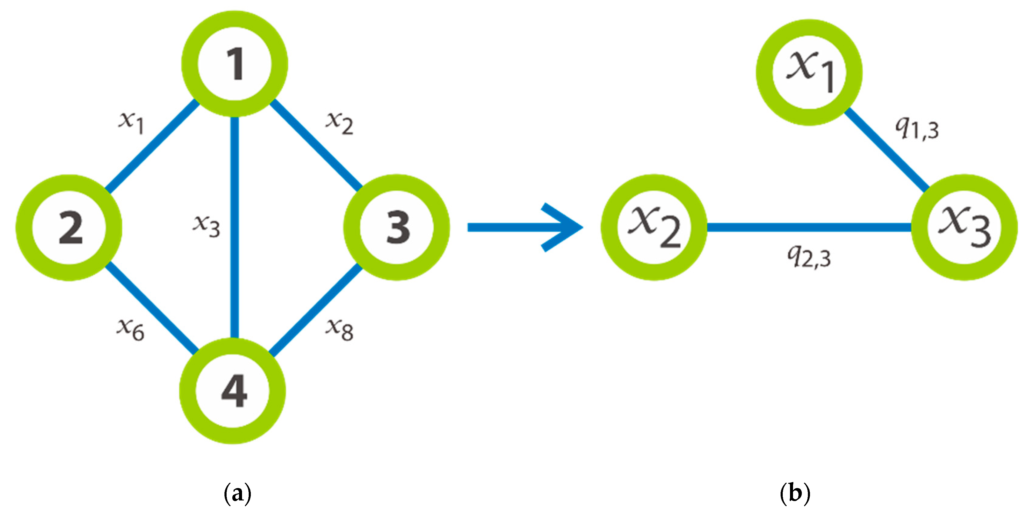
. Let us taken
as an illustration on the example for the required transformation made after we have chosen an instance of graph. Thus,
Figure 2a outlines a graph with 4 nodes which will be transformed in new graph that provided the detail on the right part of the same image. As we can see, the nodes of this new graph are labelled by
and its edges are generated by
, that formed by the edges
which having the common extremity. It is significant to notice that an edge
that symbolizes a clique of three nodes. For instance, the edge
is formed by the edges
and subsists if and only if the edge 6 (
Figure 2a) is created. In general, we consider that the set of all
is divided into
subsets where each subset includes the edges of the same level. According to
Figure 2 on the left, we can say that the set of
is divided into the first subset
which represents the edges of level 1, and all these nodes have the common extremity the node
; the second subset
which represents the edge of level 2; etc.
We could say that a clique of size possibly could be decomposed in cliques of four nodes. This also means that 4 cliques of four nodes, each two of them having two common extremities can form a clique of size .
In what follows, let
be a graph with
nodes and
edges. We assume that the least clique in this graph is a clique of five nodes (i.e.,
). The preliminary configuration of the proposed model associated to a graph
is illustrated in
Figure 3. Where
are the initial sets of objects
, the sets of enzymes associated to the layer
, and
is a enzyme associated to layers
and to layer
such that:
The system is composed by
outer layers embedded in each layer. The elementary layer, labeled 1, is associated to the node
and is included in the non-elementary layer, labeled 2 and which is included in a non-elementary layer and associated to the node
and so on, until we reach a layer labeled with
which included on its turn in a set of embedded layers labeled with
. The initial multisets consist in:
Initially, for a given graph we suppose that a graph is completely connected, i.e., we assign to each node ( edges enumerated by . Thus, each variable is considered a Boolean variable with value . This manner of operating will help us later to generate all the instances of the graph . We design by the real existing edges of an instance of the graph defining the input edges. The object is an object that will take the size of the maximal clique size in each level of each instance, and represents the possibly cliques of three nodes in each level that will be transformed in if its edges do not appear in the given base on the problem.
The set is collection of the initial enzymes associated to different layers in the system, which controlled the evolution of objects and/or layers. The enzymes can be also changed during their control base on the following set of rules that applied in a maximal parallel approach:
The first rule is based on the weak division rule for elementary layer, while the second rule is assigned to a strong division for a non-elementary layer. These rules will be used to generate all of the given graph
under the control of the enzyme
; where E and R are the limits min and max of the interval of Boolean variables
associated with the layer
, where:
After the execution of the rule , the rules (11) and (12) can provide the state of the variable by their transformation into the object (true) or into (false) meaning that the edge represented by this variable exists or not in this instance according to the enzyme presented in the layer. In all the instances where exists, indicates that this instance is not the instance that we aim to found its maximal clique. So in this moment, is changed to by applying the rule (14) that means the evolution of this subsystem is suspended.
The role of the rule (15) tends to be decreased the size of the possibility maximal clique in each level represented by the index and having the enzyme . When the marker appeared in layer , it signifies that two nodes at this level are not linked. Rule (16) will provide the specified objects and changes the enzymes according to the value of : thus, the enzyme will indicate that the value of is true and respectively will indicate that the value of is false. The rule (17) and (18) are used to check whether the current instance is the correct instance in the graph instance where the maximal clique is aimed.
This collection of rules are introduced to check the existence of (which indicate the relation between the two edges and ). Hence, according to our definition, to check that exists in an instance, we must firstly verify that and exist (i.e., they have true values), and whether this situation is true, passing on to verify their linkage. Rule (19) is devoted to eliminate all the possibly cliques of three nodes represented by having at least one of their extremities or assigned to the false value (the test is based on the presence of enzymes or ). In this case, the object will be destroyed, however, in the opposite case, the rule (20) may be applied, which consists of changing and moving to the outer layer. This is done in order to apply a second check concerning the existence of . Clearly, we say that the object maybe introduced by rule (22) whether is absent, otherwise it has a false assignment. The rule (23) sends down until it reaches the layer on the enzyme or .
This set of rules transmit and update the size of the probable maximal clique at each level according to the objects
, until when they reached the layer
, where:
This rule is part of layer dissolution rule for whether it is controlled by the enzyme , otherwise it can say that it be considered just as a cleaning rule; design empty string, where is appeared when all the possibly tests of the objects in this level are completed.
Rules (30) and (31) will be executed only if the specified condition is accomplished. In rule (29) the enzyme
in
takes the maximal clique at this level represented by the index
. The layer
can be dissolved by the execution of rule (30) in the case where the maximal clique is carried in the next level (below). Rule (31) transforms and moves the specified object that will be used later for eliminating some levels.
This set of rules consists to research the level where the maximal clique of the given graph is found. If there are several maximal cliques in different levels, the application of these rules enables at least one to be found from them.
In this part of our model, we will generate all the sets of cliques of three nodes which are able to be put together. This is done in order to construct a clique at a given level based on cliques of previous parts of our system.
These rules hold all sets of nodes where their numbers are equal to the size of the maximal clique, and eliminate all the others. When the set of nodes of the resulting maximal clique found in the layer are labeled with , the role of the dissolution layer rule (38) comes after its execution, and the provided result reach the outer layer labeled with . Finally, rule (39) evolves the enzyme to take the maximal clique.


