Numerical Analysis of the Cooling Performance in a 7.2 kW Integrated Bidirectional OBC/LDC Module

Abstract

To satisfy increasing demands for ecofriendly vehicles, researchers are now studying electric vehicle (EV)-related technologies. In particular, integrated bidirectional onboard battery charger (OBC)/low-voltage DC–DC converter (LDC) modules are being researched to improve the efficiency of onboard chargers for EV charging applications. In this study, a numerical analysis method is proposed that considers the power loss and heat flow characteristics in the design of a 7.2 kW integrated bidirectional OBC/LDC module. The developed module supports four operating modes depending on the service situation: OBC and LDC single operation, OBC/LDC simultaneous operation, and LDC operation. The mode is selected based on the power system flow. The characteristics of the circuit were analyzed in each of the four modes to compute the heat loss from the major heating elements. The results of a numerical analysis of the internal cooling characteristics showed that the internal temperature was higher in the OBC single operating mode than in the OBC and LDC simultaneous operating mode in which the power loss was the highest. The results emphasize the importance of ensuring that cooling designs consider the characteristics of various modes as well as the worst-case power loss.

1. Introduction

Until recently, the internal combustion engine was the predominant type in the automotive market. However, the ongoing depletion of fossil fuels and worsening environmental pollution is now causing this market to slowly shift toward an emphasis on ecofriendly cars with high fuel efficiency. Thus, several developed countries, such as the United States, Japan, and Europe, are now taking steps to stimulate the ecofriendly electric vehicle (EV) market and to promote the broad proliferation of charging infrastructure, which is a critical factor in the success of EVs. At the same time, much effort has been focused on improving the stability of renewable energy sources and supporting the decentralization of energy.

A major area of focus with regard to EV technologies is to provide components and systems that are high-performance, lightweight, and stable. In particular, development efforts are currently focused on advancing battery technology, such as high-performance, high-density energy storage technologies, and electric drive systems, including high-voltage electrical components, high-power drive motors, and motor control technologies, all of which are core technologies for EVs. Furthermore, to simplify the control and electrical systems in EVs and reduce the overall cost, modules are now being developed that integrate several previously disparate functions into one assembly. One example of this trend is the integration of power conversion devices to increase their efficiency and improve their performance.

Researchers currently working in the area of integrated power converters are focusing on a variety of circuit improvements [1,2,3]. For example, onboard chargers (OBCs) and low-voltage DC–DC converters (LDCs) are being researched as a way to overcome space limitations and poor fuel economy of systems with connected batteries [4,5,6,7]. These integration efforts are seeking to leverage high-efficiency circuit structures using miniaturized, lightweight components, such as switch-mode power supplies (SMPSs). Studies are also underway to solve the low reverse recovery charge problem using a GaN element with a totem-pole structure in continuous current mode (CCM) operation [8,9]. Another example is the use of high-frequency switching signals using an insulation-type converter, such as a series-loaded resonant DC–DC converter (SRC) or LLC resonant converter, to minimize power loss in the DC–DC converters commonly used for the auxiliary charging of EVs by applying [10,11,12,13]. In addition, as cooling performance has become an important consideration in circuit improvement, experimental methods of evaluating the cooling performance of heating elements are also being researched [14]. Note that such studies typically employ experimental methods instead of the numerical methods commonly used in battery pack design [15].

Recently, the Buck Converter of the two-way charging system has been proposed as an optimization control method considering the State of Charging (SOC) [16,17,18,19,20] and the State of Healthy (SOH) [21,22,23], and the research is being actively conducted. Among the SOC methods, the CC–CV (Constant Current/Constant Voltage) method, which is the simplest basic model and is controlled according to the determined voltage and current [16], and the CVCC–CV (Constant Voltage/Constant Current/Constant Voltage) and MCC–CV (Multi-Stage Constant Current/Constant Voltage) have been proposed for fast charging and securing cycle stability [17,18]. On the basis of this, a study has been performed on the converged models. For example, CC–CV and MCC–CV have been converged to consider variables such as charging speed and energy conversion efficiency [19,20]. In addition, under high temperature conditions, the battery surface may exceed the allowable temperature depending on the state of charge and discharge, resulting in a negative performance such as battery life cycle and charging acceptance. The method considering SOH has been proposed as a method for checking battery life and water solubility to improve performance degradation problems and stability problems due to overheating, and research for checking the effects of temperature, energy efficiency, and battery aging has been carried out [22,23].

In previous studies, efforts have been made to improve circuit efficiency and improve cooling performance. However, most of the previous studies are designed considering only specific conditions or conditions for main modes. The power conversion device used in this study operates in various modes depending on the situation, and the circuit characteristics change accordingly, so it is necessary to consider the design stage to cope with this. In particular, the 7.2 kW integrated bidirectional onboard battery charger/low-voltage DC–DC converter (OBC/LDC) module is very intensively designed in order to increase power density; thus, it is indispensable to understand the characteristics of each operation mode to effectively dissipate heat generated from internal circuits. In this study, a numerical analysis method is proposed that considers the power loss and heat flow characteristics in the design of a 7.2 kW integrated bidirectional OBC/LDC module. In addition, the cooling system design takes into account changes in the heating characteristics depending upon the operating modes.

A 7.2 kW integrated bidirectional OBC/LDC module for an EV consists of four main parts: A totem-pole power factor correction (PFC), series resonant converter, high-voltage buck converter, and low-voltage buck converter. Each part is composed of an inductor to induce a voltage in proportion to the current change rate, a diode that rectifies the current by allowing it to flow in only one direction, a metal–oxide–semiconductor field-effect transistor (MOSFET), which is a type of transistor that performs amplification and switching by adjusting the current or voltage flow, and a transformer that increases or lowers the AC voltage via the mutual inductance principle. The main sources of heat in this type of module are the diode, rectifier, and inductor, and the heat generated from these devices has the potential to degrade the performance and safety of the system if not properly handled.

Thus, the arrangement, cooling method, and operating conditions are critical factors in the stable performance of the power converter. In addition, it is essential that the cooling performance be examined in light of the heat generated by each element and its supporting structure. The conventional approach to the cooling problem involves numerical analyses with the objective of minimizing the internal temperature of each device, while considering the heat value produced by each major heat source to be constant. However, as the size and position of the heat sources in the proposed 7.2 kW integrated bidirectional OBC/LDC module varies depending on the operating mode, the conventional approach cannot be used in that design.

To overcome this limitation, a numerical analysis method is introduced to support a cooling system design that supports changes in the operating mode of the module. The proposed method involves an unsteady state analysis to determine the changes in the circuit and heat flow in each operating mode. Then, the obtained circuit heating and internal cooling characteristics are analyzed based on the numerical results.

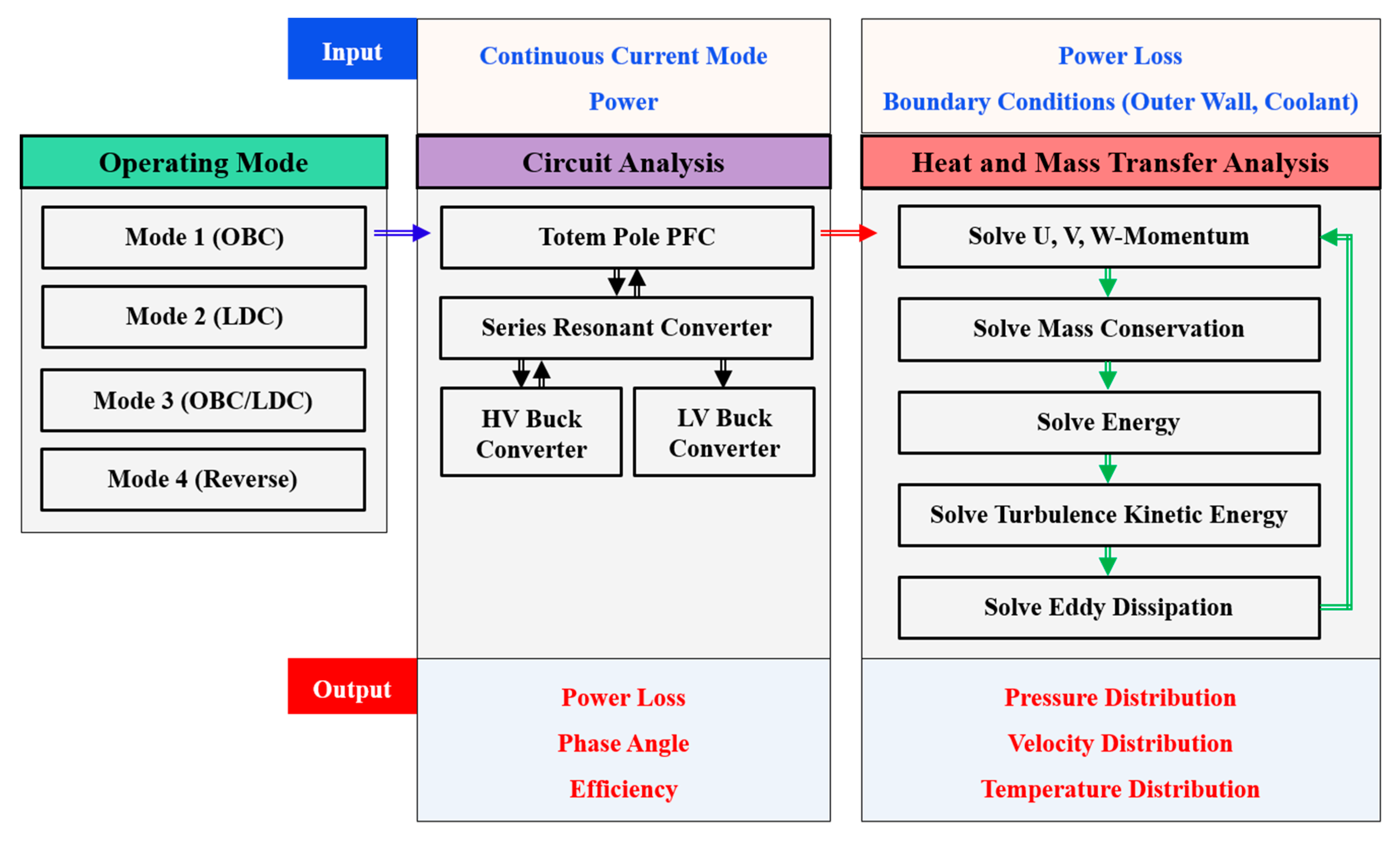
The circuit and heat flow analysis method used in this study are depicted in Figure 1. The circuit was configured based on the results of the numerical analysis, and the power loss and efficiency were then calculated in each operating mode (Modes 1 to 4) using MATLAB/Simscape. The calculated power loss of each device was then converted to a heating value and used in the subsequent analysis. A heat flow analysis model constructed in the ANSYS Fluent 19.2 software package was used in the evaluation of the cooling performance. The circuit characteristics of each operating mode of the module were analyzed using the results, and the cooling performance was then validated based on the computed internal heating characteristics.

2. Development of the Numerical Model

2.1. Circuit Simulation Model of the Integrated Module

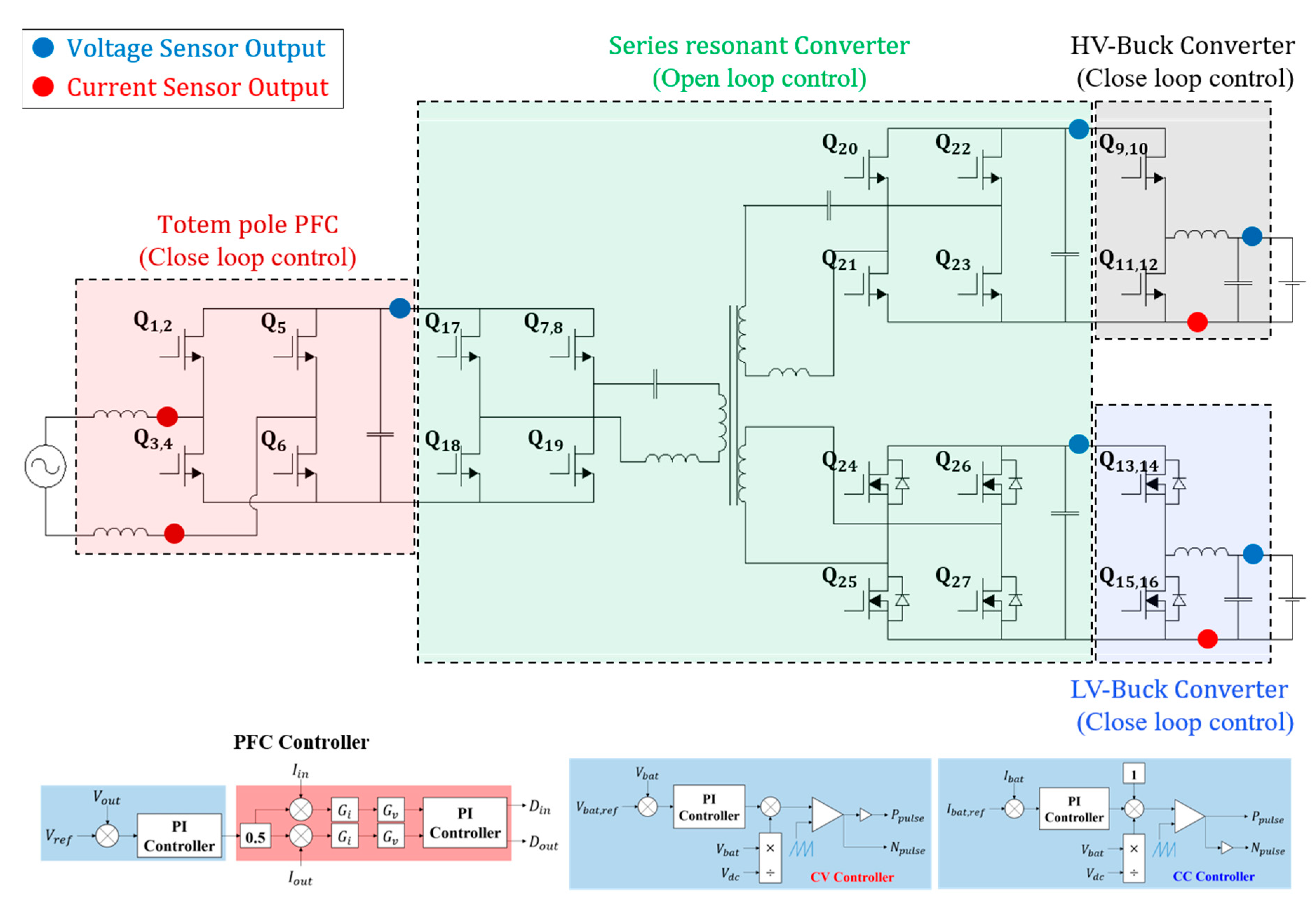
A circuit diagram of the developed 7.2 kW integrated bidirectional OBC/LDC module is shown in Figure 2. In this circuit, the totem-pole PFC and buck converter were implemented as bridgeless and synchronous rectification types, respectively. These operate as follows: When the AC voltage is positive, the PFC stores energy in the inductor and switches Q3–Q5 are turned on. Later, when Q3–Q5 are switched off, the energy stored in the inductor is discharged and the current flow passes through switches Q1–Q2 and Q6. The PFC control block is configured based on the duty cycle of the current (Equation (1)) and the voltage–current (Equation (2)) relationships as follows [24]:

$$G_i=\frac{i_L}{d}=\frac{C{V}_{DC}+2(1-D)I_L}{(LC)s^2+\left(\frac{L}{R}\right)s+{\left(1-D\right)}^2}\approx \frac{V_0}{sL},$$

(1)

$$G_v=\frac{v_o}{i_L}=\frac{\left(1-D\right)V_{DC}-L{I}_L}{C{V}_{0}s+2(1-D)I_L}\approx \frac{1}{sC{V}_0}.$$

(2)

The DC-DC converter in the circuit is represented as a series resonant converter (SRC) in which the primary and secondary circuits are separated using a transformer. In the forward direction, the AC voltage is converted to a DC voltage using switches Q7 and Q8, whereas in the reverse direction, the voltage is converted using switches Q20–Q23. The output voltage in the forward direction is determined by the high- or low-battery-voltage setpoints, which depend on the winding ratio, resonance point, and operating frequency of the transformer. This circuit was designed to generate a constant output voltage by aligning the resonance point and operating frequency to 300 kHz. In addition, the system was configured to respond to a broad range of output voltages depending on the number of windings.

The SRC resonance-type circuit is configured through a serial connection with a transformer ratio of 12:14:1, based on the output in the high- and low-voltage directions at the primary side. The equivalent model was constructed based on this configuration. The output voltage can be predicted as follows [25]:

$$V_{convert}=G_{sw.g}{G}_{resonant.g}{N}_s/N_p,$$

(3)

The resonant gain graph of the SRC resonant circuit can be defined as follows. Note that the m value was omitted because, unlike the LLC circuit, the SRC circuit has only one inductor:

$$G_{resonant.g}=\frac{F_x^2(m-1)}{\sqrt{1+jQ{\left(\frac{1}{F_x}-F_x\right)}^2}}$$

(4)

where $F_x$ is the ratio of the resonance frequency and switching frequency and Q (Equations (5) and (6)) is the quality factor, which is defined as follows:

$$Q=\frac{\sqrt{L_r/C_r}}{R_{ac}},$$

(5)

$$R_{ac}=\frac{8}{{\pi }^2}\frac{N_s^2}{N_p^2}{R}_L.$$

(6)

Using Equations (4) to (6), the resonant gain of the SRC circuit can be expressed as shown in Figure 3, where the maximum output voltage can be 467 V. Therefore, it is necessary to control the step-up and step-down through the introduction of the buck converter to stabilize the battery.

The buck converter reduces the voltage based on the output voltage of the DC–DC converter. The inductor voltage is applied when the switch turns on and the amount of current increases. In contrast, when the switch turns off, the operating mode disconnects the input power. The control block of the buck converter circuit maintains a high stability by enabling constant current (CC) operation during charging. Then, when discharging, the constant voltage (CV) control method is used instead to improve the overall efficiency.

2.2. Simulation of the Operating Mode

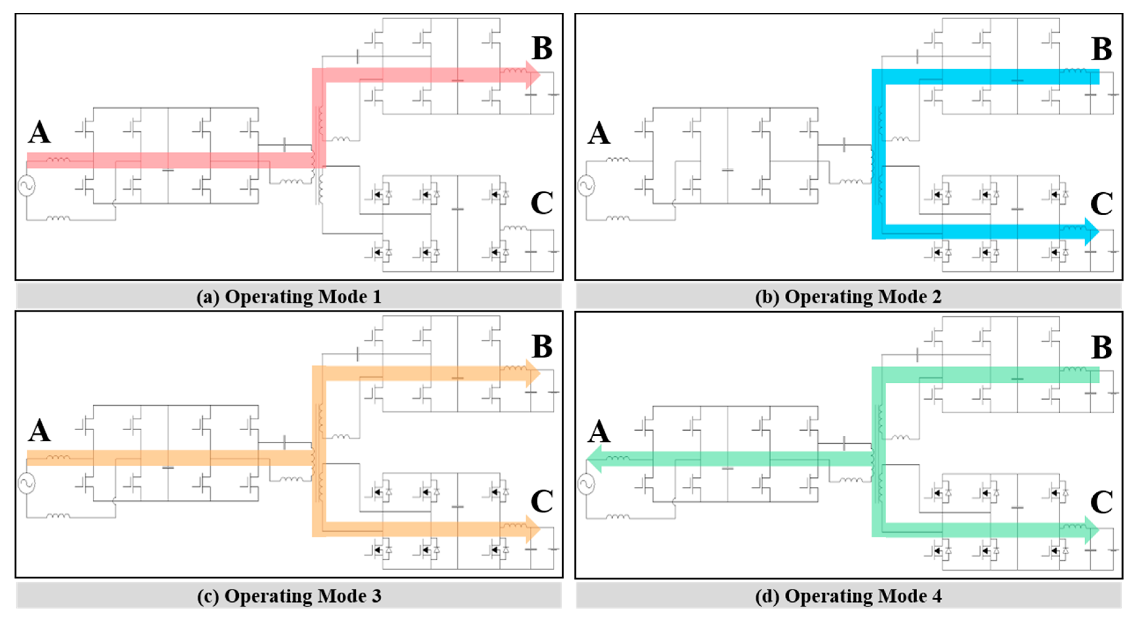
As shown in Figure 4, the bidirectional integrated circuit has four operating modes: OBC or LDC single operation, LDC operation, or simultaneous operation of the OBC and LDC in forward and backward directions.

In Operating Mode 1, the OBC operates independently and the vehicle remains stationary. The LDC does not operate in this mode because the low-voltage battery is sufficiently charged. When compared to a driving situation, the total load of the circuit in this mode is significantly lower.

In Operating Mode 2, the LDC operates independently. In this mode, the low-voltage battery is charged by the high-voltage battery, while the vehicle is driving. Under driving conditions, the 12 V battery has 80% load. The OBC circuit does not operate without the AC charge cable connected, and the power flows from the high-voltage battery toward the LDC circuit. Consequently, the maximum power of the LDC in independent operation is 2.5 kW.

Operating Mode 3 is defined as the simultaneous activation of the OBC and LDC circuits when the low- and high-voltage batteries are not sufficiently charged. This mode provides enough additional power to operate the controllers in the EV, such as the engine control unit (ECU) and battery management system (BMS). In total, an output power of 6.9 and 0.3 kW can be generated in the OBC and LDC circuits, respectively.

Operating Mode 4 is defined as the time when power flows from the high-voltage battery to power the system and the LDC. This occurs when the EV is stationary. In this mode, output powers of 3 and 0.3 kW can be generated in the OBC and LDC circuits, respectively.

Using these definitions of the operating modes, the heat loss in each mode was predicted by simulating the circuit. The heat loss over time for each of the major heating elements was derived, and the values were applied to the heat flow model to analyze the cooling characteristics in the integrated module.

2.3. Numerical Model

A numerical model was constructed to verify the heat flow characteristics of the 7.2 kW integrated bidirectional OBC/LDC module. Note that this model contained a simplified representation of the module that included only the major heating elements. This approach was adopted as the remaining elements had only a small impact on the heat flow characteristics. In addition, the bolts or nuts used to mount the outer structure in the EV were ignored.

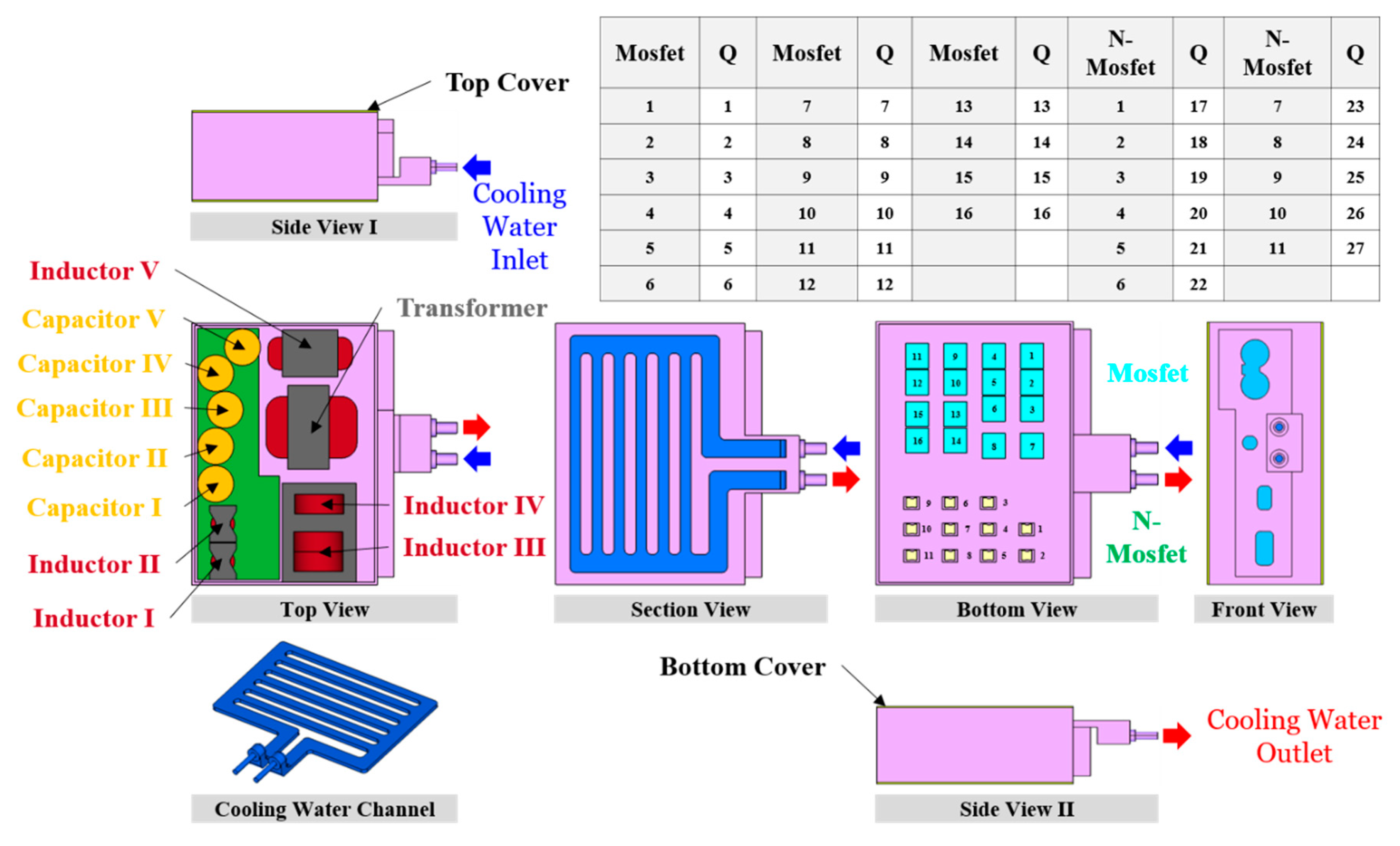
The configuration and shape of the integrated module from several perspectives are illustrated in Figure 5. This was used when mounting the module in a vehicle, which was the objective of the analysis in this study. The module body is composed of a top cover, main body, and bottom cover. There is an OBC circuit inside the top cover, which is sealed to protect the internal devices. Inside the main body, there is internal support for the OBC/LDC circuits and a cooling channel for recovering heat from the device. These components are also sealed to protect the internal devices.

The parts inside the module that generate the most heat are six inductors, one transformer, 16 MOSFETs, and 11 N-MOSFETs. The heating value of each device was estimated in the previously described circuit simulation and varies depending on the mode.

Cooling water is injected into the inlet and flows along the parallel channels to recover heat from the heating elements. In the numerical model, the heat is assumed to be transferred from the components to the cooling water via natural convection through the air layer inside the charger. When evaluated, this approach provided a result close to that of the actual model.

To verify the flow characteristics of the integrated module, a flow and heat transfer analysis was performed. To accomplish this, a three-dimensional model of the simplified charger was constructed and an unsteady-state analysis was performed to observe the initial temperature changes inside the charger. The physical properties of the body of the charger and the internal fluid were assumed to be constant, and it was also assumed that heat was generated uniformly in each heating element area. Based on these assumptions, the governing equations for the flow and heat transfer analysis were as follows:

• Mass conservation equation

  $$\frac{\partial \rho }{\partial t}+\nabla \cdot \left(\rho \overrightarrow{u}\right)=0.$$

  (7)
• Momentum conservation equation

  $$\frac{\partial \left(\rho \overrightarrow{u}\right)}{\partial t}+\nabla \cdot \left(\rho \overrightarrow{u}\overrightarrow{u}\right)=-\nabla p+\nabla \cdot \left(\mu \nabla \overrightarrow{u}\right).$$

  (8)
• Transport equation for κ (standard k-ε model)

  $$\frac{\partial \left(\rho k\right)}{\partial t}+\nabla \cdot \left(\rho k\overrightarrow{u}\right)=\nabla \cdot \left[\left(\mu +\frac{{\mu }_t}{{\sigma }_k}\right)\nabla k\right]+G_k+G_b-\rho \epsilon .$$

  (9)
• Transport equation for ε (standard k-ε model).

  $$\frac{\partial \left(\rho \epsilon \right)}{\partial t}+\nabla \cdot \left(\rho \epsilon \overrightarrow{u}\right)=\nabla \cdot \left[\left(\mu +\frac{{\mu }_t}{{\sigma }_{\epsilon }}\right)\nabla \epsilon \right]+C_{1\epsilon }\frac{\epsilon }{k}\left(G_k+G_{3\epsilon }{G}_b\right)+C_{2\epsilon }\rho \frac{{\epsilon }^2}{k}.$$

  (10)
• Energy conservation equation

  $$\frac{\partial \left(\rho C_{p}T\right)}{\partial t}+\nabla \cdot \left(\rho C_{p}T\right)=\nabla \cdot \left(k_{eff}\nabla T\right)+S_e.$$

  (11)

First, the fluid flow was analyzed by solving the continuity and momentum equations. Then, the equation describing the k-ε standard model was solved to account for the turbulence caused by the high Reynolds number of the fluid (Re = 7453). Next, the energy conservation equation was solved to determine the heat transfer to the internal heating elements and the surroundings. Finally, to model the natural convection inside the charger, the air density was calculated assuming the air was an incompressible ideal gas.

2.4. Properties and Boundary Conditions

To determine the heat flow characteristics inside the integrated module when mounted in a vehicle, the model used physical properties and boundary conditions that were identical to those of the actual device. First, the solid properties of the external charger (aluminum), inductor (copper), diode (plastic), transformer (steel + copper), and printed circuit board (PCB) of the charger were defined. Then, the physical properties of a fluid were assigned to the internal air and cooling water. The values of the physical properties are listed in

Table 1. Physical properties of the components and materials in the integrated module.

Description		Density [kg/m3]	Viscosity [Pa-s]	Specific Heat [J/kg-K]	Thermal Conductivity [W/m-K]
Fluid	Water	998.2	1.003 × 10−3	4182	0.600
	Air	variable	1.789 × 10−5	1006	0.024
Solid	Aluminum	2719	-	871	202.4
	Copper	8978	-	381	387.6
	Diode	1190	-	1465	0.190
	PCB	1890	-	600	0.810
	Steel	8030	-	502	16.3

. In the case of the inductors and diodes, although these devices contain various materials, the physical properties were selected based on the representative element that occupied the largest part. Furthermore, although the actual physical properties of the various components varied with temperature, these factors were ignored because they were assumed to be small.

The boundary conditions of the integrated module are listed in

Table 2. Boundary conditions used in the numerical analysis model.

Condition		Value	Unit
Inlet	Velocity	2.17	m/s
	Temperature	300	K
Outlet	Outlet Pressure	-	-
Outer Wall	Temperature	300	K
	Convection Heat Transfer Coefficient	10	W/m2-K
Heat Source	Uniform Heat Source	variable	W/m3

. The inlet velocity applies to the cooling water inlet used for system cooling. The cooling water flow rate of 6 LPM in an actual operating charger was converted to velocity for use in the analysis. The outlet pressure refers to the pressure at the cooling water outlet to ensure that the circulating water can be discharged without encountering resistance. Most of the heat generated in the integrated module is removed via the circulating cooling water, and the remainder is discharged to the atmosphere via convection as the external surface is exposed to air. Therefore, a convection condition was allocated to the external surface (300 K, h = 10 W/m²-K) in the model to represent the heat being discharged to the outside air. Furthermore, the internal air is circulated via natural convection based on the temperature difference (density difference), which results in heat diffusion. To simulate this, the air density (assuming an incompressible ideal gas) was calculated based on the temperature, which was used to specify the heat transfer by natural convection considering the effects of gravity. The results of the previous circuit simulations were used to determine the heating value of each part and device in this model.

2.5. Numerical Procedures

A numerical analysis was conducted using the above governing equations and boundary conditions together with the ANSYS Fluent 19.2 software package. During the analysis, the internal temperature variation over time and the internal temperature changes in each operating mode were assessed. Specifically, the cooling performance based on the size of the heat source in each mode was monitored and evaluated relative to the maximum temperature of each device. The convergence criterion for solving the continuity, momentum, and energy equations was 10.6. To evaluate the grid dependency, an analysis was conducted for grid sizes from 4,480,000 to 10,230,000, and it was determined that stable results could be achieved at a grid size of 7,840,000.

3. Results and Discussion

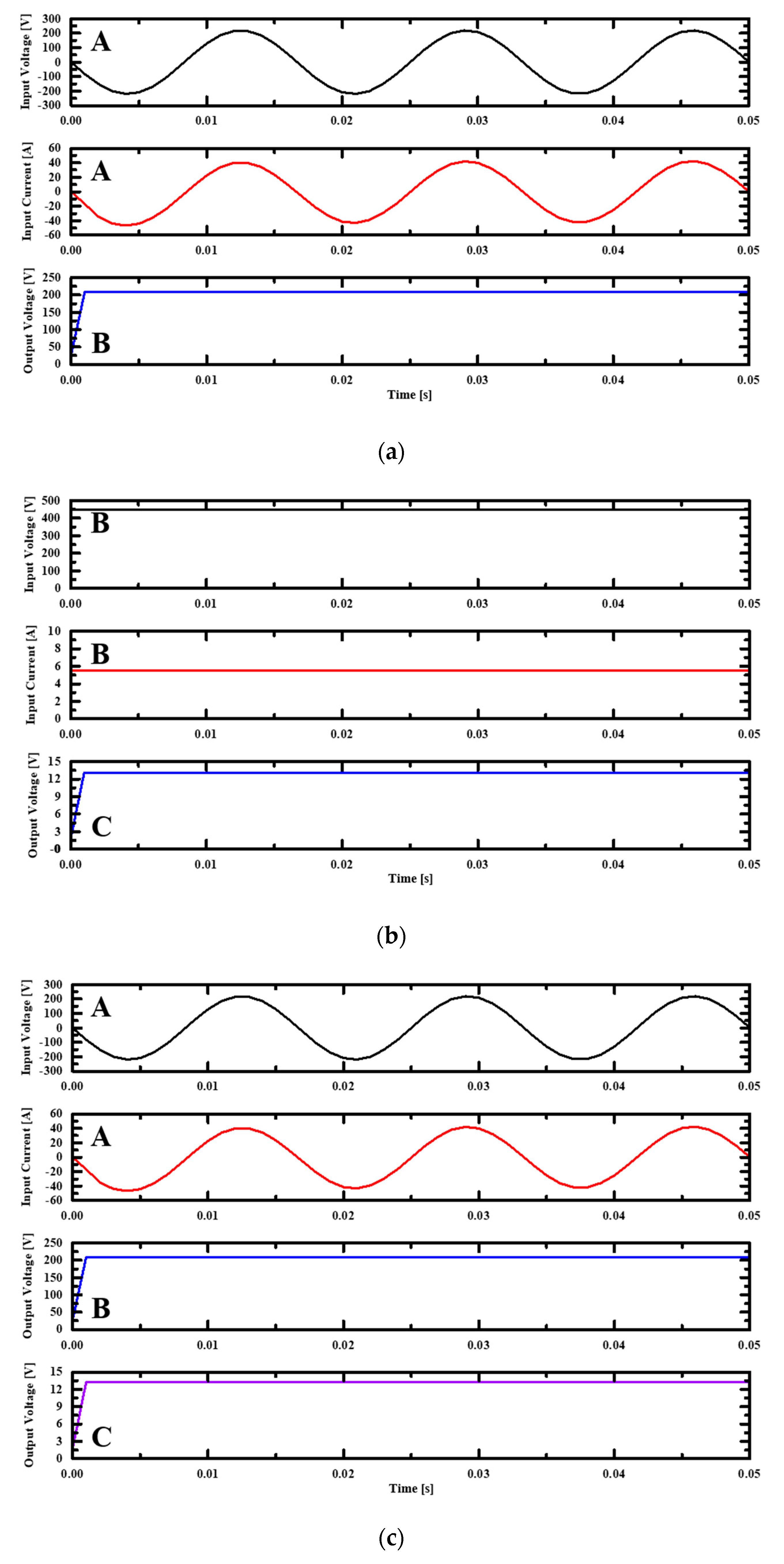
A circuit analysis was conducted using the circuit diagram shown in Figure 2. In terms of the system power, power was supplied using CCM. Graphs representing the input voltages applied during the simulation and the corresponding output voltages derived through the analysis are shown in Figure 6a,c. Here, the applied input voltage and current were 85–265 V and 32 A, respectively. The control block ensured that the input/output voltages were similar in every mode.

For the PFC circuit, the control block minimized the phase angle to produce a DC output voltage of 400 V. Furthermore, the fixed output voltage in the SRC circuit was predicted to be 470 V when the resonant frequency was aligned to the operating frequency. This value is similar to that predicted using the gain function.

The operation of the buck converter varied depending on the high- and low-voltage battery conditions. A simulation was conducted for a state of charge (SOC) of 0%, and the results are shown in Figure 6b,d. In the figures, it can be seen that output voltages of 220 and 13 V occurred at the ends of the high- and low-voltage buck converters, respectively. Furthermore, when the charge state continued, the current was fixed under CC control, and the output voltage increased to 450 V at the high-voltage end. In the discharge state, a fixed voltage was maintained under CV control. Here, the input voltage in Operating Modes 2 and 4 was 450 V.

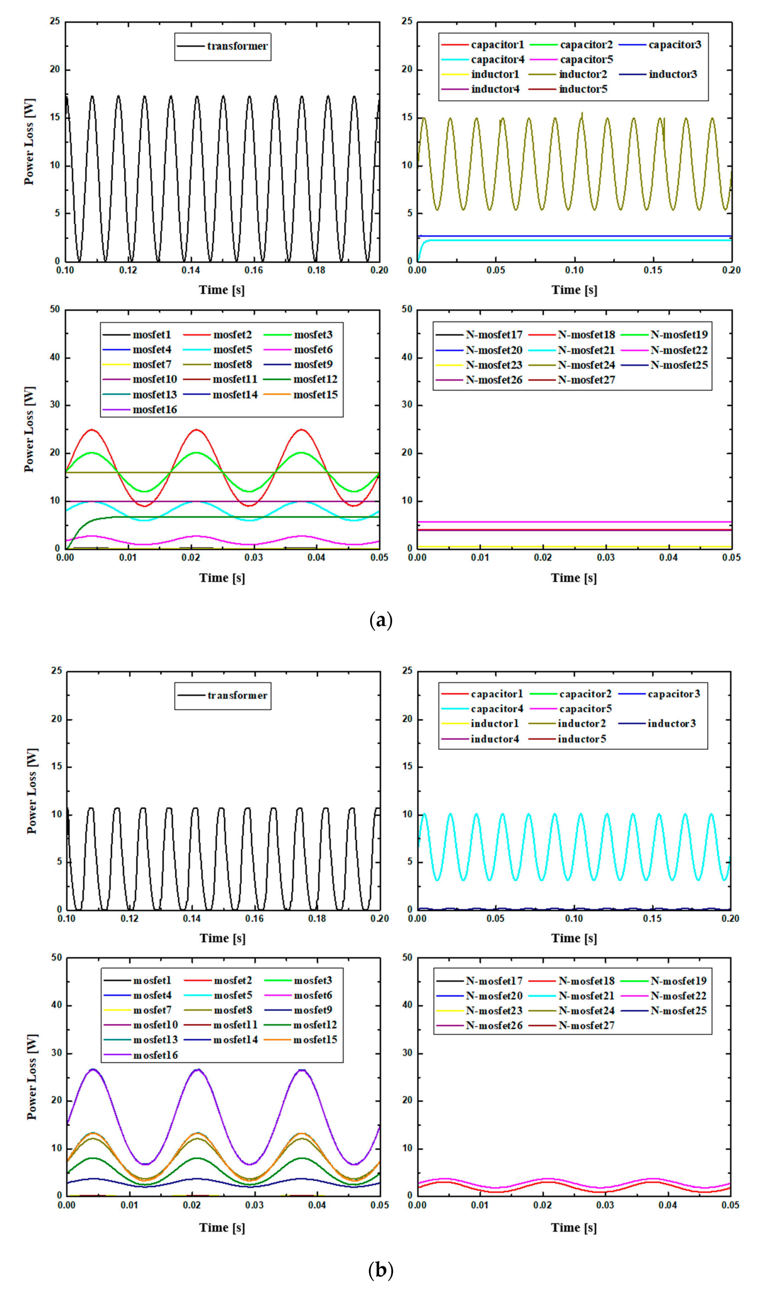
The proposed integrated module has four operating modes, and the power loss of each is shown in Figure 7. In each mode, the output power ranged from 2.5 to 7.5 kW, and the MOSFET device generated the largest loss in all modes. First, Operating Mode 1 (Figure 7a) represents the independent operation of the OBC circuit, while the LDC circuit is deactivated when the low voltage battery is in a fully charged condition. In this mode, the total power loss in the PFC, SRC, and buck converter circuits were 94 W, 73 W, and 32 W, respectively. This indicates that the amount of supplied current in each circuit had a significant effect on the power loss.

In Operating Mode 2 (Figure 7b), 2.5 kW of power flowed from the high-voltage battery to the low-voltage battery, which necessitated a large amount of power to be allocated to the LDC circuit compared to that in the other operating modes. In the high-voltage buck converter, the voltage remained constant as the circuit was under CV control, while the current decreased somewhat, which resulted in a smaller power loss than in Operating Modes 1 and 3. However, in the low-voltage buck converter, the power supply increased eight times, and the power loss increased relative to that of other operating modes.

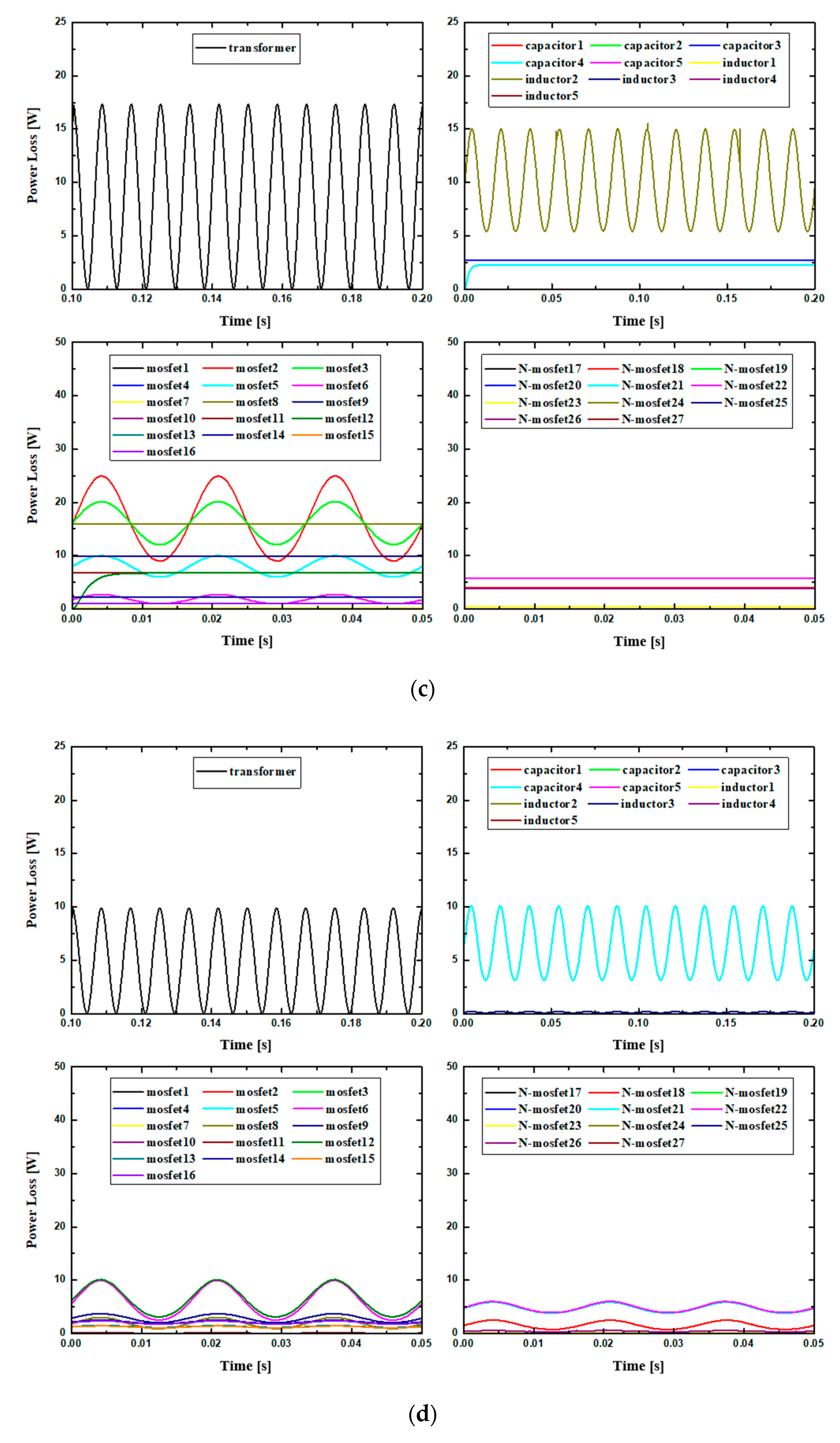
In Operating Mode 3 (Figure 7c), which denotes OBC/LDC simultaneous charge mode, a power of 7.2 kW was supplied, of which 6.9 and 0.3 kW were allocated to the OBC and LDC circuits, respectively, depending on the load of the controller. Since the power distribution was the same as that of Operating Modes 1 and 4, the loss of each circuit was also similar. In total, an efficiency of 96.99% was realized in Operating Mode 3.

In Operating Mode 4 (Figure 7d), 3.3 kW of power flowed backward from the high-voltage battery to the system power and onward to the low-voltage battery. This backward flow produces a different power loss depending on the reverse recovery time of the active devices and the size of the reverse bias voltage, although the loss is smaller than that in the forward direction. In total, the efficiency of Operating Mode 4 was computed to be 96.75%.

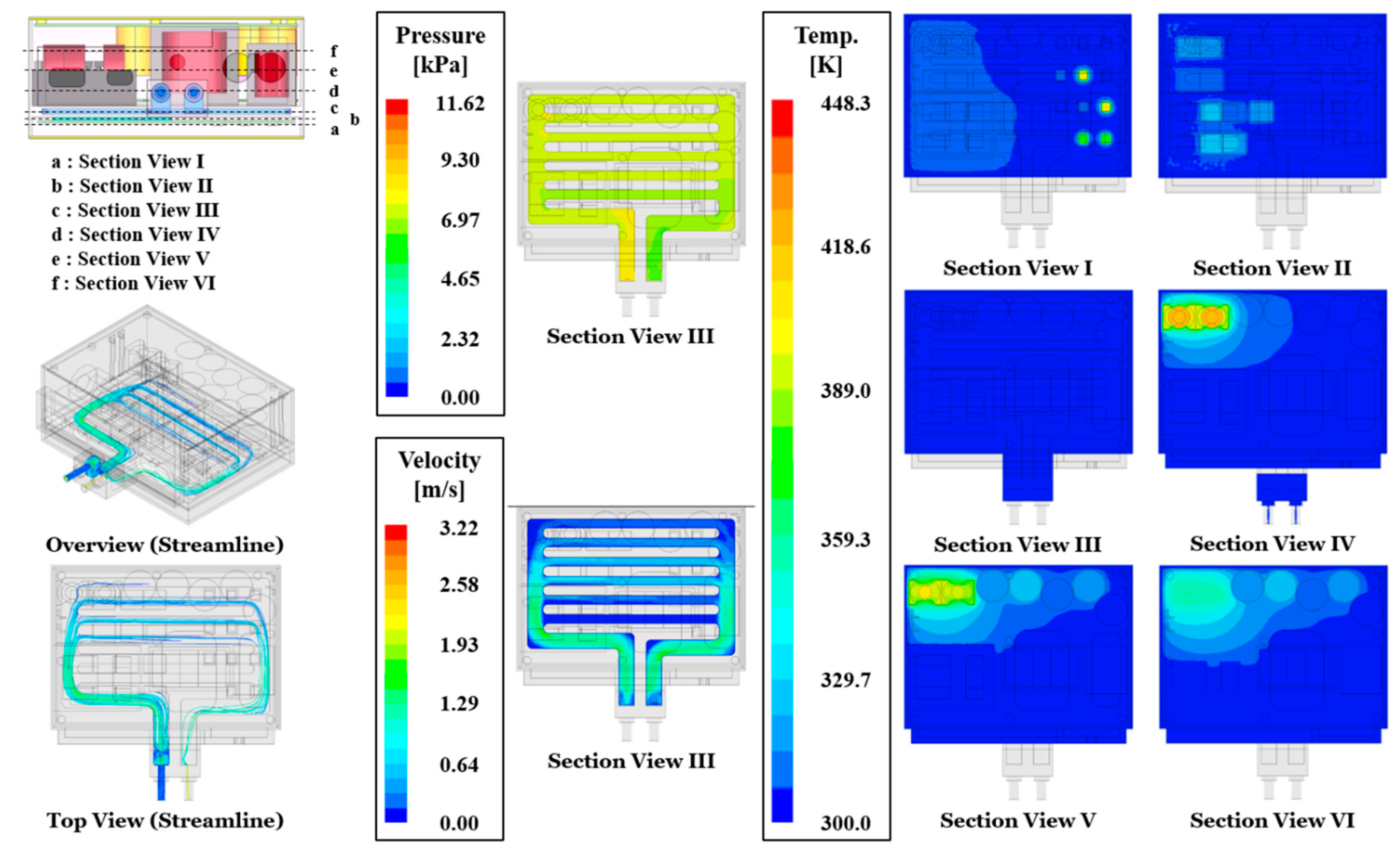
The results of the heat flow analysis are shown in Figure 8, Figure 9, Figure 10, Figure 11, Figure 12, Figure 13, Figure 14 and Figure 15 for the various operating modes. 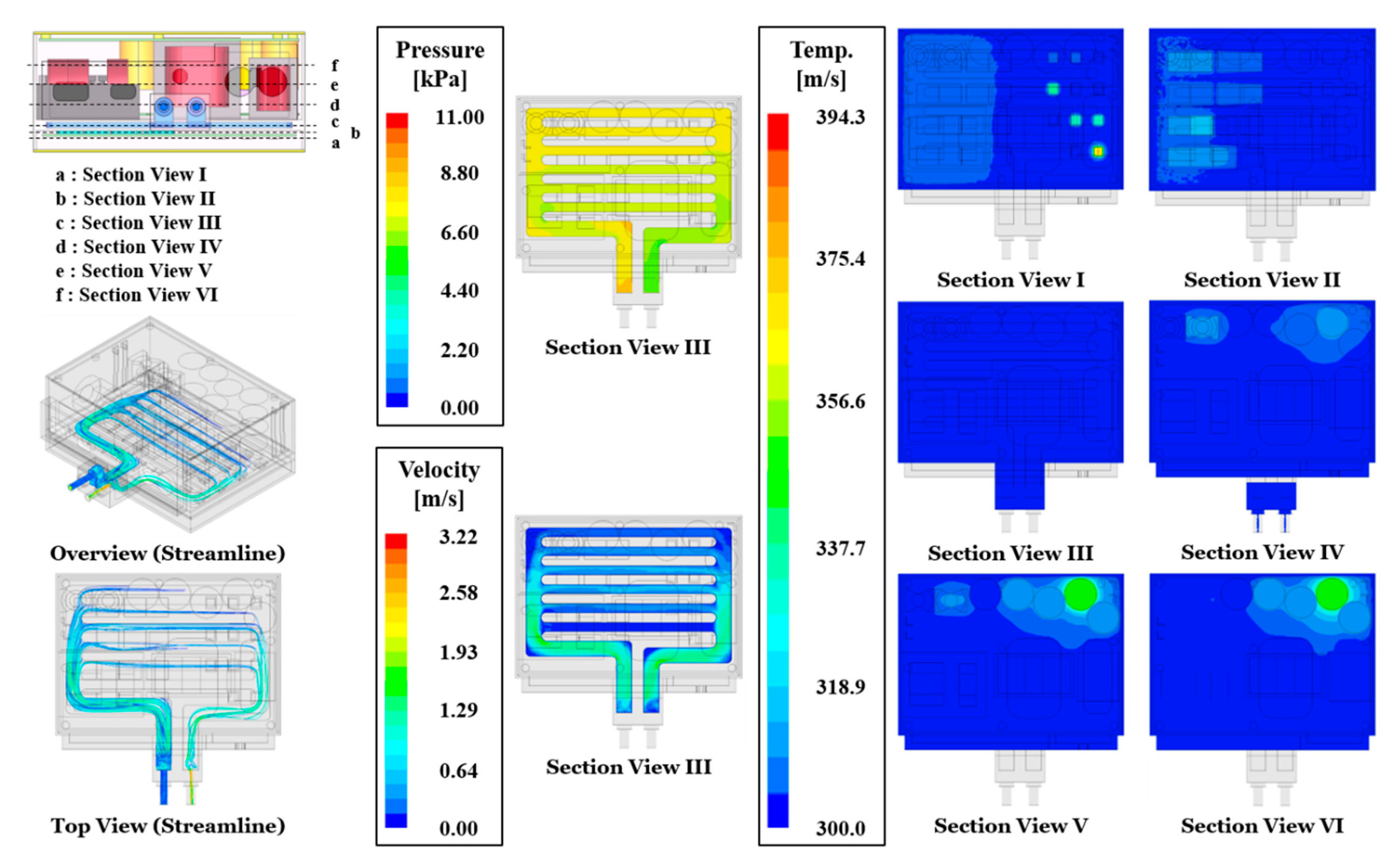The conditions for this analysis included a cooling water flow of 6 LPM in the forward direction (left inlet, right outlet), and to simulate the exposure of the charger module to air, the convection conditions on the external surface were set to 300 K and h = 10 W/m²-K. To confirm the heat flow characteristics for each operating mode, the results of streamline, pressure, velocity, and temperature distributions over a time period of 4000 s were evaluated. The streamline distribution was identified using a top-view drawing. The pressure and velocity characteristics were identified by drawing the cross-section of a cooling channel through which the fluid flows (Section View III in Figure 8). The temperature distribution was evaluated based on the locations of the major devices. In Figure 8, Section View I (a) shows the center position of the cooling water channel, Section Views IV (d) and V (e) show the center position of the inductor, and Section View VI (f) shows the center position of the capacitor.

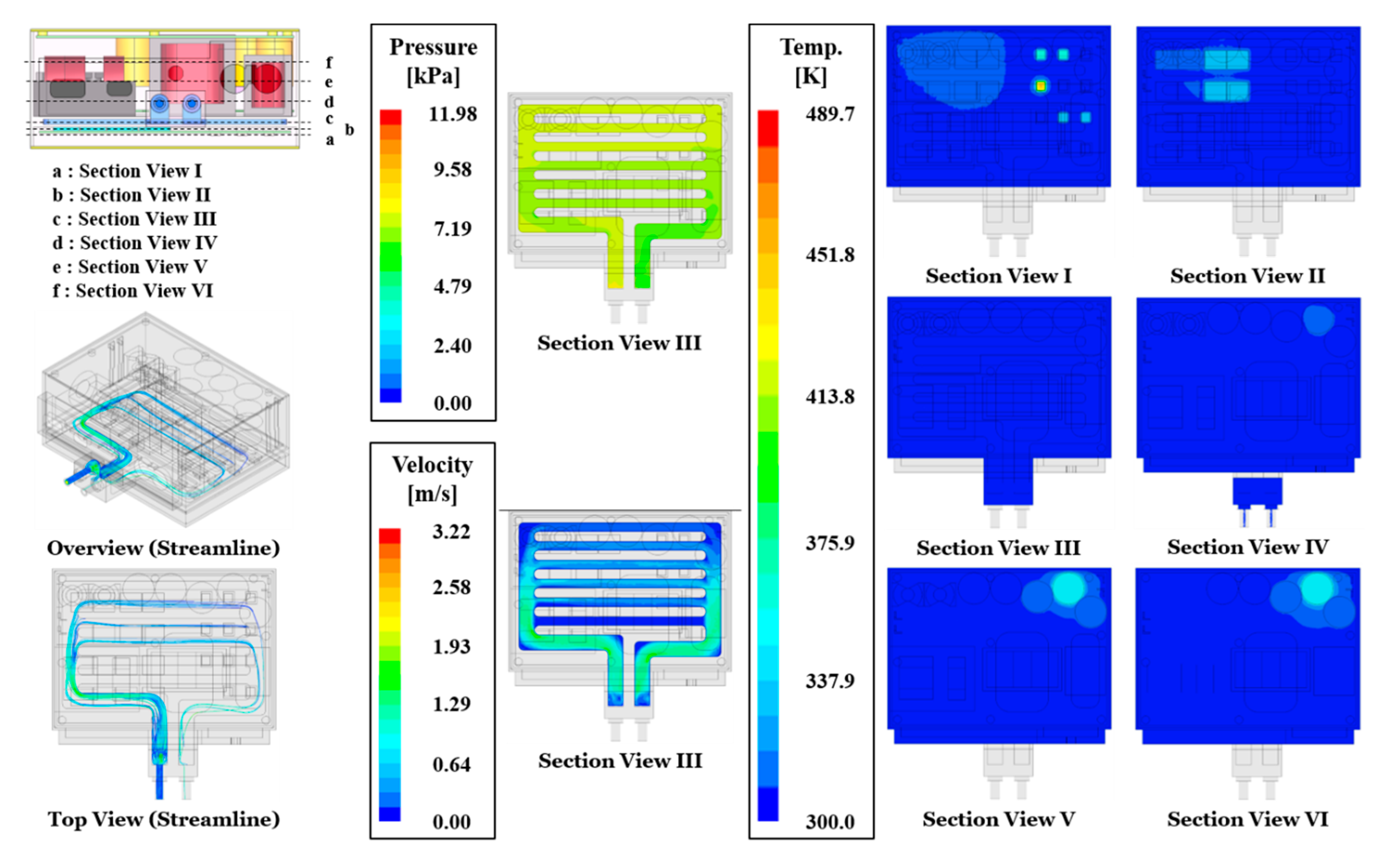
The results of analyzing Operating Mode 1 are shown in Figure 8. The streamline, pressure, and velocity distributions shown in the figures were used to verify the flow characteristics of the cooling water. The streamline distribution shows that the fluid was injected into the inlet, passed through the internal channel, and flowed out the outlet. As the water flowed through the module, the heat from the heat sources was transferred to the cooling water, and then flowed out through the outlet and away from the module. The pressure distribution in the cooling water channel was predicted to be the highest at the inlet and to drop by 11.62 kPa as it flowed through the channel. A high velocity distribution with a small cross-sectional area was seen in the inlet and outlet channels on the bottom of the module with a relatively low velocity distribution in the center where the majority of the heating sources were concentrated.

A limitation was identified in this analysis in that the parallel configuration of the cooling water channels introduces variations in the velocity distribution of each channel, depending on the degree of flow distribution. This should be improved by adjusting the channel layout as the current configuration degrades the heat transfer coefficient and heat transfer rate. In the future, we plan to conduct a follow-up study to optimize the cooling performance, based on the results of this study.

In terms of the temperature distribution, the highest temperatures in Section View I were observed in N-Mosfet XXI (410.9 K) and XXIII (410.5 K). In Section View II, the highest temperatures were observed in Mosfet II (320.3 K), Mosfet III (319.5 K), Mosfet V (319.6 K), and Mosfet VIII (318.2 K). In Section Views III and IV, the highest temperatures were observed in Inductor I (422.6 K) and Inductor II (417.7 K). In Section View V, the highest temperatures were observed in Capacitor I (319.9 K), Capacitor II (326.1 K), and Capacitor IV (318.7 K). These results were produced by the circuit load associated with SRC operation in Operating Mode 1 in which the OBC operates independently. Note that the results varied as the operating mode changed. In other words, the operating circuit domain is affected by the operating mode, which changes the heating elements and the heating value.

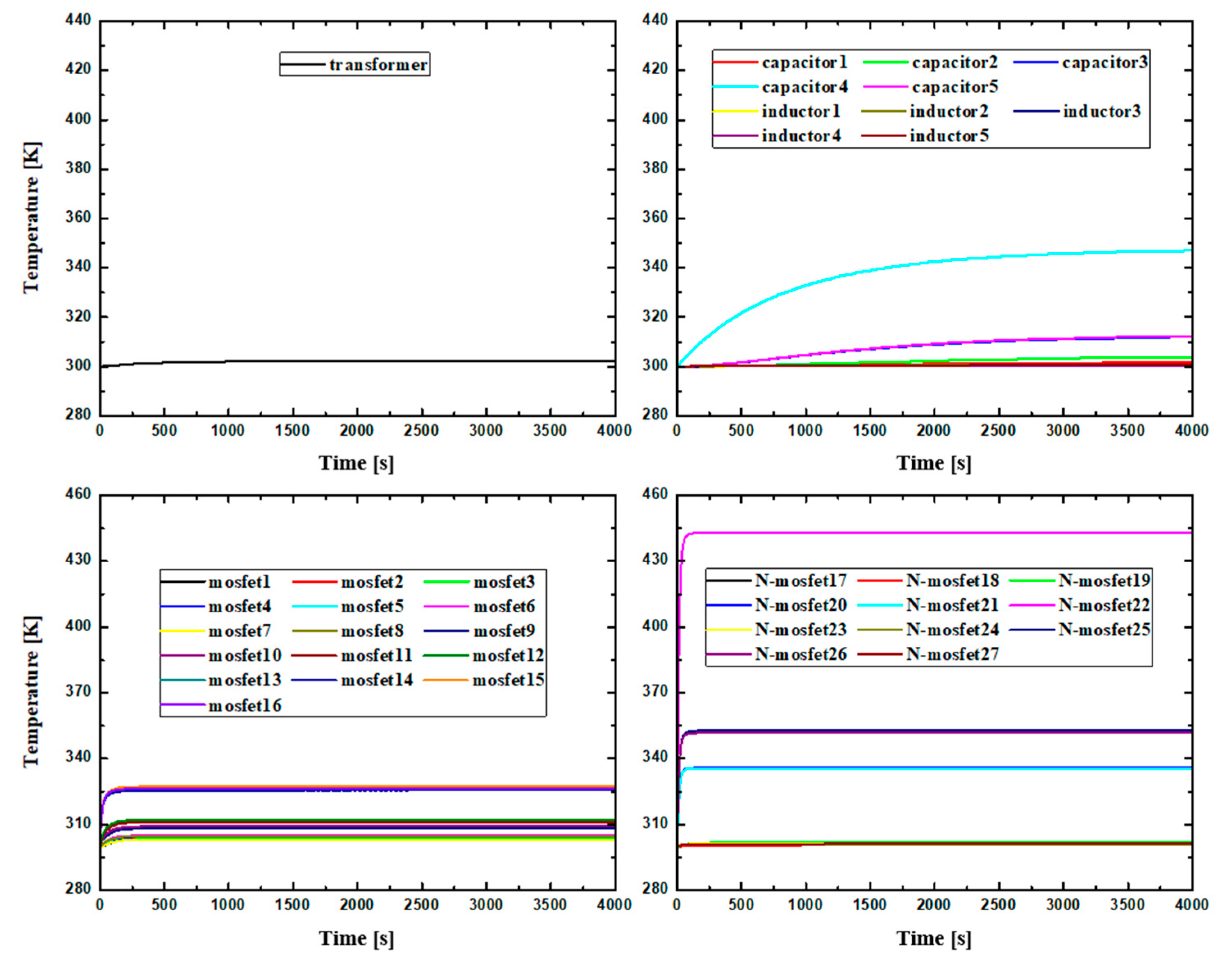
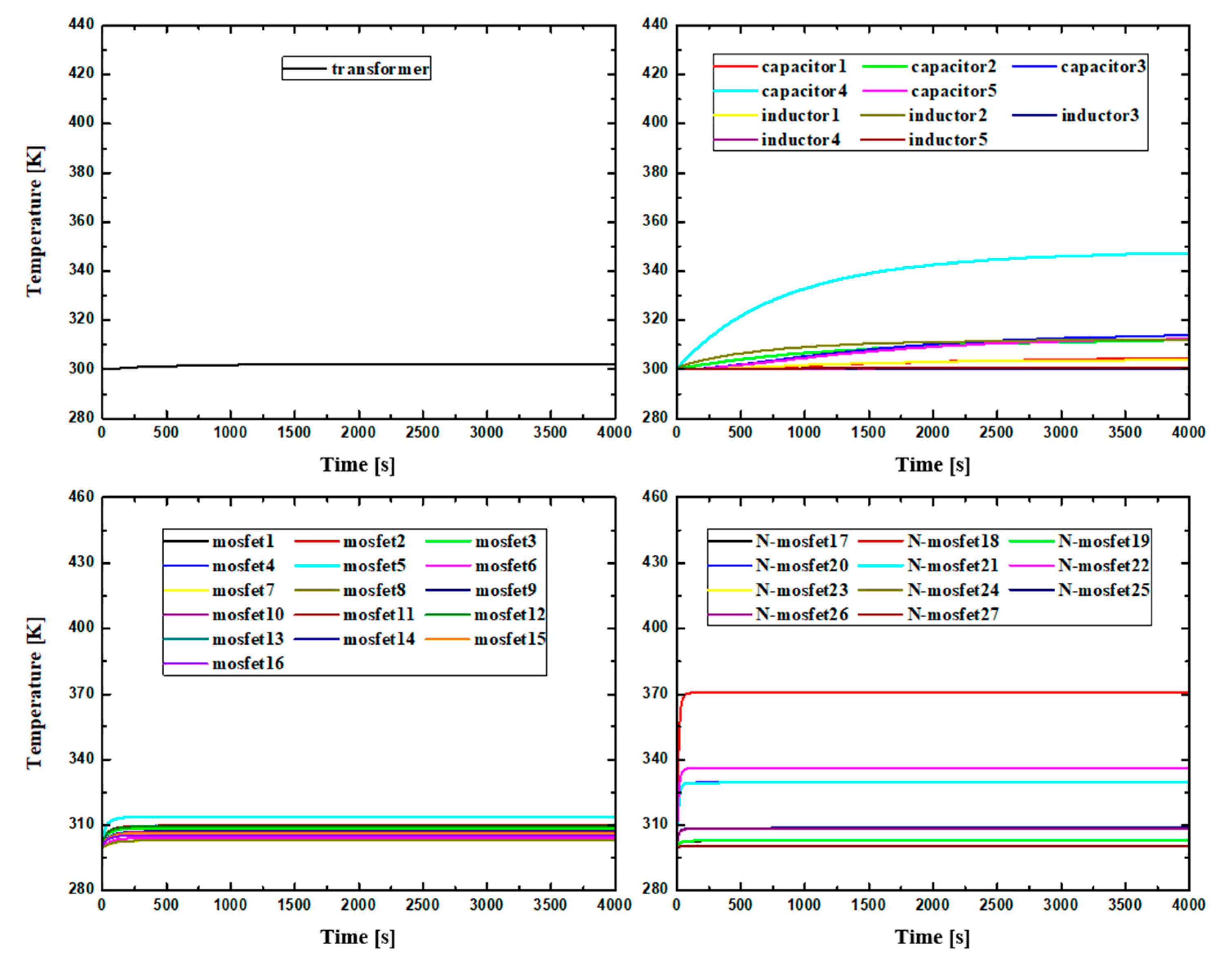
The internal temperature changes over time in Operating Mode 1 are shown in Figure 9, where it can be seen that for Mosfet and N-Mosfet, which are relatively small devices, the temperature of the circuit after startup quickly rose until it stabilized at around 200 s. However, in the case of the transformer, inductor, and capacitor, which have relatively large volumes, the temperature curve is gentle and it takes a long time to reach steady state. In other words, as Mosfet and N-Mosfet have a larger heat source or heating value per unit volume (W/m³), the temperature rapidly rises until it reaches steady state. In the future, to prevent these devices with large heat sources from reaching their critical temperature, the cooling design should reflect the circuit characteristics and operating mode as well as the required durability of each device.

When the charging rate of the low-voltage battery for vehicle control becomes too low, the LDC operates independently (Operating Mode 2). This configuration is shown in Figure 10. When the streamline is examined to identify the characteristics of the cooling water, it can be seen that a streamline formed along a channel shape similar to that in Operating Mode 1 with the same behavior. In addition, the predicted velocity and pressure distributions were similar to those in the previous case. In terms of the numbers, the highest pressure distribution appeared at the inlet, and the pressure drop through the system was predicted to be 11.98 kPa. With regard to the temperature distribution for each section, in Section View I, the highest temperature was observed in N-Mosfet XXII (443.0 K). In Section View II, the highest temperatures were observed in Mosfet XIII (326.2 K), Mosfet XIV (325.6 K), Mosfet XV (327.4 K), and Mosfet XVI (326.5 K). In Section Views III and IV, no device exhibited a particularly high temperature. In Section View V, the highest temperature was observed in Capacitor IV (347.1 K). As explained above, these results were produced using a circuit load consistent with the independent operation of the LDC in Operating Mode 2. Thus, the cooling system design should be based on N-Mosfet XXII, which exhibited the highest temperature. Note that it is important that the cooling system be improved because the predicted temperature of 443.0 K is high enough to affect the durability of the device.

The internal temperature changes over time in Operating Mode 2 are shown in Figure 11. As shown, for relatively small devices, such as Mosfet and N-Mosfet (i.e., devices with a large heat source in terms of the heating value per unit volume (W/m³)), the temperature rises quickly from startup until it converges to steady state at around 200 s. In the case of the transformer, inductor, and capacitor (all devices with a small heat source in terms of the heating value per unit volume (W/m³)), the temperature curve is relatively gentle. Therefore, in the design of the cooling system for Operating Mode 2, the circuit characteristics and operating mode should be such that the N-Mosfet XXII is prevented from reaching the critical temperature.

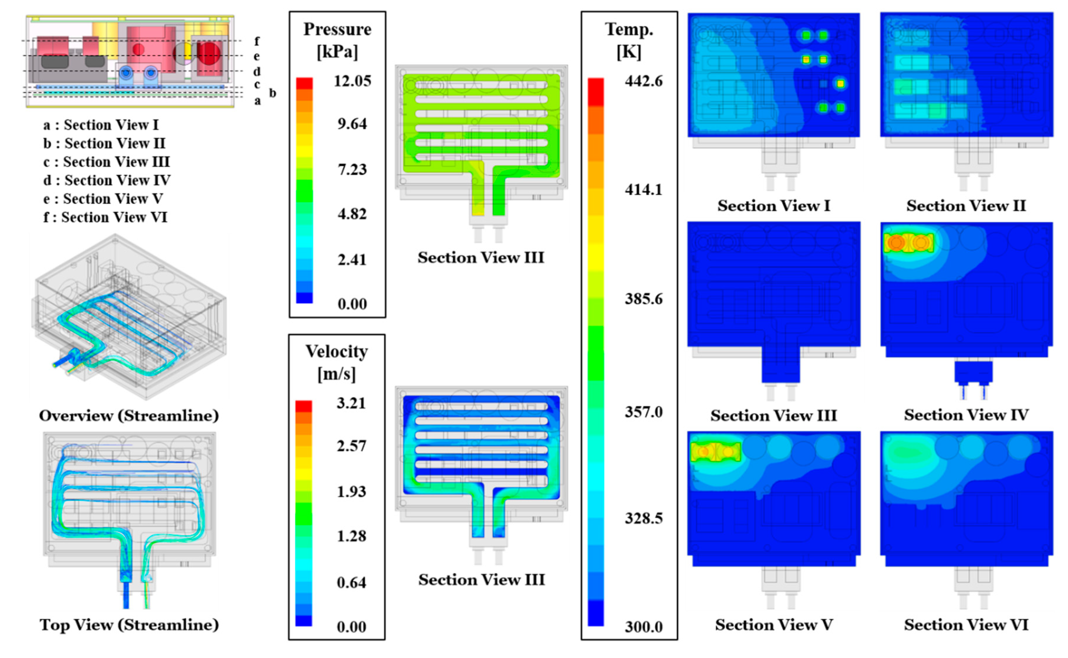
The results of the analysis conducted in Operating Mode 3 are shown in Figure 12. Note that in this mode, the OBC and LDC are simultaneously activated when the low-voltage and high-voltage batteries do not have sufficient energy stored. The predicted streamline, velocity, pressure distributions, and flow characteristics of the cooling water were similar to those in the previous cases. The highest pressure distribution was predicted to be at the inlet with an overall pressure drop of 12.05 kPa through the system. In terms of the temperature distribution for each section, in Section View I, the highest temperatures were observed in N-Mosfet XVII (375.5 K), N-Mosfet XVIII (374.9 K), N-Mosfet XXI (406.7 K), N-Mosfet XXII (407.9 K), N-Mosfet XXIII (399.7 K), N-Mosfet XXV (373.4 K), and N-Mosfet XXVI (372.4 K). In Section View II, the highest temperatures were observed in Mosfet I (330.3 K), Mosfet II (330.1 K), Mosfet III (340.0 K), Mosfet IV (342.4 K), Mosfet IX (331.8 K), and Mosfet X (330.4 K). In Section Views III and IV, the highest temperatures were observed in Inductor I (423.2 K) and Inductor II (418.4 K). In Section View V, the highest temperatures were observed in Capacitor I (320.3 K), Capacitor II (325.8 K), and Capacitor IV (319.6 K). The overall temperature trend was similar to that of Operating Mode 1. As the OBC and LDC were activated simultaneously and both low-voltage and high-voltage batteries were charged, the trends in this mode were similar to those of the OBC independent operation mode.

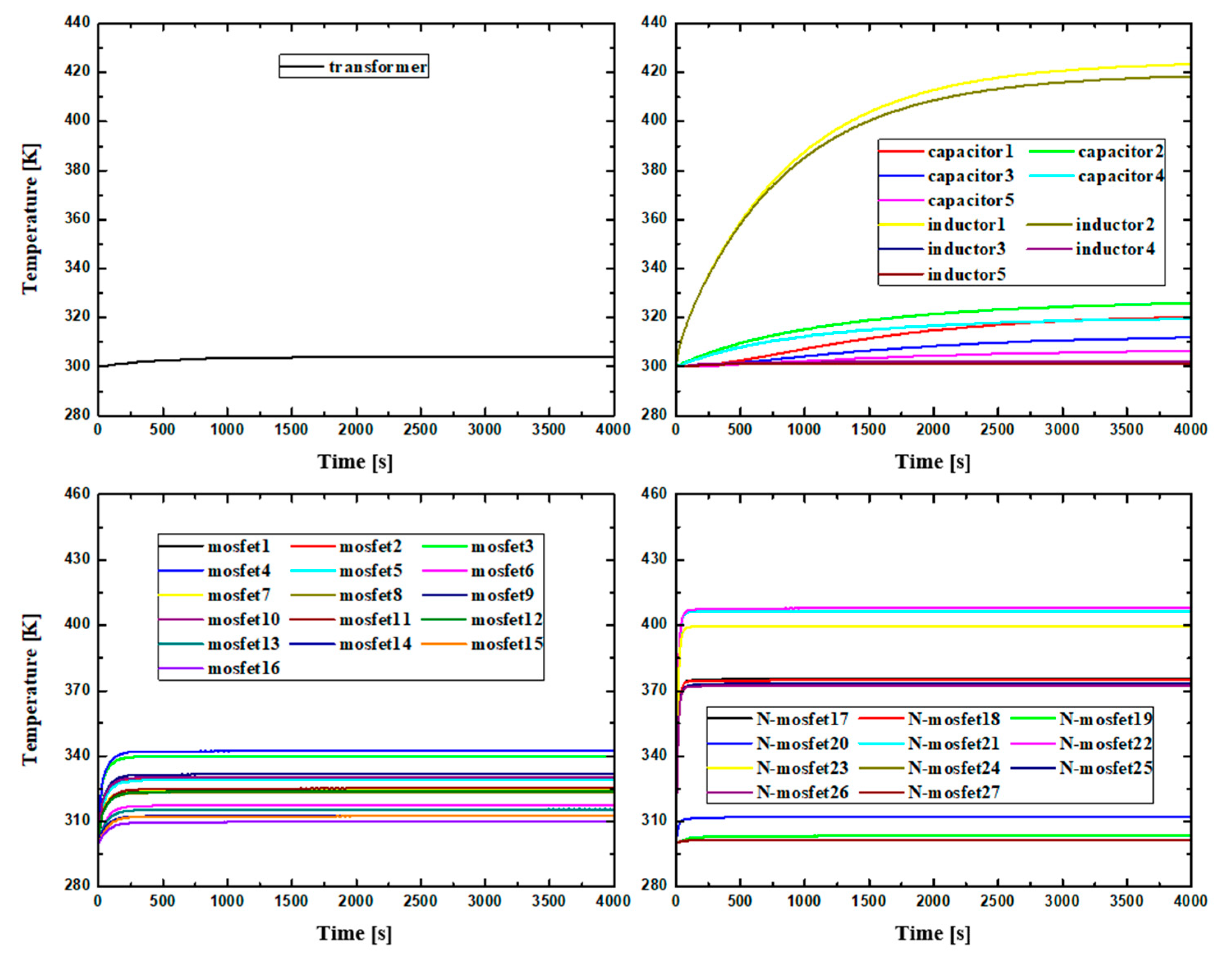
The internal temperature changes over time in Operating Mode 3 are shown in Figure 13. The shape of the temperature rise differs depending on the size of the heat source in terms of the heating value per unit volume (W/m³). When compared to Operating Mode 1 (448.3 K), the highest temperature in the module decreased to 442.6 K. This was likely because the power was distributed when both the OBC and LDC were charged, compared to the case when only the OBC was in use for the same power source. Thus, the loss in the circuit was lower.

The results of analyzing the circuit in Operating Mode 4 are summarized in Figure 14, where it can be seen that the power flows from the high-voltage battery to the system power and LDC in this configuration. The predicted streamline, velocity, pressure distributions, and flow characteristics of the cooling water were similar to those in the previous cases. The highest pressure distribution was located at the inlet, and a pressure drop of 11.00 kPa was predicted in the system. In terms of the temperature distribution for each section, in Section View I, the highest temperatures were observed in N-Mosfet XVIII (370.7 K), N-Mosfet XX (329.7 K), N-Mosfet XXI (329.6 K), and N-Mosfet XXII (336.4 K). In Section View II, the highest temperatures were observed in Mosfet I (309.6 K), Mosfet II (309.4 K), Mosfet III (308.6 K), and Mosfet IV (314.0 K). In Section Views III and IV, the highest temperature was observed in Inductor II (312.2 K). In Section View V, the highest temperature was observed in Capacitor IV (347.4 K). The overall predicted temperature was lower than that in the other modes (394.3 K), which is because the thermal load generated from the loss was based on output powers in the OBC and LDC circuits of 3 and 0.3 kW, respectively, when the power flowed from the high-voltage battery to the system power and LDC. The internal temperature changes over time in Operating Mode 4 are shown in Figure 15. Note that the predicted temperature curves differed depending on the size of the heat source in terms of the heating value per unit volume (W/m³) of each device.

The results demonstrated that the locations and heating values of the heating elements vary depending on the operating mode of the integrated module. Thus, it is essential that the cooling system design is optimized accordingly. In other words, the design must consider the circuit characteristics, operating mode, and required durability of each device to prevent any device from reaching its critical temperature.

4. Conclusions

A numerical analysis methodology for the circuit and heat flow characteristics of a 7.2 kW integrated bidirectional OBC/LDC module with different operating modes was presented, based on which the following conclusions were obtained. First, a numerical analysis model for the loss rate of an electric circuit was proposed, and the calculated loss rate was adjusted based on the heating value. This value was supplied as an input to the heat flow analysis process to determine the equilibrium state of the temperature distribution. When analyzed, the electrical circuit and heat flow characteristics of the module were changed based on the operating mode, which affected which circuits were activated. The power losses in the operating modes were approximately 142 and 196 W, respectively, when the LDC and OBC were operated independently. However, in a high-voltage/low-voltage charging mode in which both the OBC and LDC were activated, the power loss was the highest at approximately 216.36 W. Furthermore, in Operating Mode 4, in which the power flows from the high-voltage battery to the system power and LDC, the power loss was the lowest at approximately 107 W.

To examine the thermal characteristics, in Operating Mode 1, where the OBC operates independently, the highest temperatures were observed in N-Mosfet XXI (410.9 K), XXIII (410.5 K), Inductor I (422.6 K), and Inductor II (417.7 K). In terms of the changes in the internal temperature over time, in the devices with a large heat source in terms of the heating value per unit volume (W/m³), such as Mosfet and N-Mosfet, the temperature rose quickly until it reached steady state (around 200 s). However, in the case of the transformer, inductor, and capacitor, it took much longer to reach steady state because the temperature rise curve was gentle. In Operating Mode 2, in which the LDC operates independently, the highest temperature was predicted in N-Mosfet XXII (443.0 K). In Operating Mode 3, where the OBC and LDC are activated simultaneously, the highest heating value was generated in many devices. However, as the power was distributed, the heating temperature in the circuit decreased to 442.6 K, compared to 448.3 K in Operating Mode 1. Thus, it is essential that the cooling design for the integrated module consider the cooling characteristics in different modes as well as the characteristics of the mode with the largest power loss.