Joint Spatial-Spectral Smoothing in a Minimum-Volume Simplex for Hyperspectral Image Super-Resolution

Abstract

The limitations of hyperspectral sensors usually lead to coarse spatial resolution of acquired images. A well-known fusion method called coupled non-negative matrix factorization (CNMF) often amounts to an ill-posed inverse problem with poor anti-noise performance. Moreover, from the perspective of matrix decomposition, the matrixing of remotely-sensed cubic data results in the loss of data’s structural information, which causes the performance degradation of reconstructed images. In addition to three-dimensional tensor-based fusion methods, Craig’s minimum-volume belief in hyperspectral unmixing can also be utilized to restore the data structure information for hyperspectral image super-resolution. To address the above difficulties simultaneously, this article incorporates the regularization of joint spatial-spectral smoothing in a minimum-volume simplex, and spatial sparsity—into the original CNMF, to redefine a bi-convex problem. After the convexification of the regularizers, the alternating optimization is utilized to decouple the regularized problem into two convex subproblems, which are then reformulated by separately vectorizing the variables via vector-matrix operators. The alternating direction method of multipliers is employed to split the variables and yield the closed-form solutions. In addition, in order to solve the bottleneck of high computational burden, especially when the size of the problem is large, complexity reduction is conducted to simplify the solutions with constructed matrices and tensor operators. Experimental results illustrate that the proposed algorithm outperforms state-of-the-art fusion methods, which verifies the validity of the new fusion approach in this article.

1. Introduction

Hyperspectral images (HSIs) with high spatial resolution play an increasingly important role in feature extraction and terrain classification of the underlying materials [1,2,3]. However, hyperspectral sensors have some limitations regarding spatial resolution, such as hardware and technology. Furthermore, the spatial and spectral resolutions are closely linked; i.e., better spectral resolution automatically leads to coarser spatial resolution and vice versa. Therefore, it is very difficult to obtain high-spatial-resolution HSIs directly. As an effective and economical approach to image enhancement or super-resolution, fusion of hyperspectral and multispectral images (MSIs) has attracted extensive attention in remote sensing, and substantial research results have emerged [4,5]. Nevertheless, there are still many problems to be solved [1,4,6], such as spatial resolution, spectral distortion and anti-noise performance.

Pansharpening, originally designed to solve the fusion of MSIs and panchromatic images, can be adapted to handle the fusion of HSIs and MSIs using the classical information processing methods [5], such as the component substitution method [7,8] and multi-resolution analysis [9,10]. For example, the component substitution method [8] constructed the spectral band mapping between the MSI and clustered HSI, and then replaced the spatial component of the HSI with the corresponding part of the MSI for the reconstructed image. The multi-resolution-analysis-based pansharpening methods [7] linearly combined multispectral band images to synthesize a high-spatial-resolution image for each HSI band. However, these methods do not fully exploit the intrinsic relationship between the HSI and MSI, which often results in serious spectral distortion and performance degradation. In addition, with the development of artificial intelligence, there are many fusion algorithms based on deep neural networks [11,12,13]. For example, Yang et al. [11] proposed a fusion method based on a deep convolutional neural network (CNN) with two branches for HSI and MSI separately, by exploiting spectral correlation. Multi-branch back propagation neural networks were employed by Han et al. [13] to propose a cluster-based fusion method to address the non-linear spectral mapping for each cluster. Generally, supervised learning needs a training database based on images or pixels.

Data fusion aims at integrating the observed low-spatial-resolution HSI data and high-spatial-resolution MSI data to obtain the reconstructed super-resolution image with high spatial and spectral resolutions. Conversely, the observed HSIs and MSIs can be regarded as spectral and spatial degradation of the high-spatial-resolution HSI, which is called the observation model. Data fusion is often an inverse problem, made so by fusing the observed HSI and MSI data to enhance the spatial resolution of reconstructed images. Furthermore, the inverse problem of data fusion is ill-posed. To address the difficulties, Bayesian-based methods dedicated to the fusion of HSIs and MSIs have been designed, which adopted the priors (e.g., Guassian prior) to design the algorithms in the principal component subspace or wavelet domain [14]. Another popular approach is hyperspectral super-resolution (HySure) [15], in which the fusion problem was reformulated by introducing the vector-total-variation regularization into convex data fitting terms, and was solved by the split augmented Lagrangian shrinkage algorithm. In addition, the research by Wei et al. [16] developed a Bayesian-based sparse representation (BSR) method, in which a proper posterior distribution was refined by the decomposition of the image on a set of dictionaries. However, this kind of fusion method typically involves a high computational load, so some measures were taken to reduce the large computational complexity of Bayesian-based fusion approaches; for example, a Sylvester equation-based fast fusion [17].

As is well known, HSIs and MSIs are both cubic data, which can be considered three-dimensional tensors. Recently, another category of state-of-the-art method has been developed on basis of tensor decomposition, and includes canonical polyadic decomposition (CPD) [18,19] and Tucker decomposition [20,21,22], which can retain the cubic structure information of remote sensing images. For example, Li et al. [20] proposed a fusion algorithm based on coupled sparse tensor factorization (CSTF), which was reformulated as the iterations of a core tensor and dictionaries of the three modes. Charilaos et al. [19] brought forward a CPD-based fusion framework, in which the identifiability of the reconstructed image was discussed under mild conditions. Wang et al. [22] proposed a tensor-based approach to handle the problem of HSI spatial super-resolution by incorporating the regularizers of nonlocal low-rank tensor approximation and total variation. However, as the rank-1 version of Tucker decomposition [23], CPD is usually used to describe linear local features in the image, rather than complex features. In NMF-based hyperspectral unmixing, the data can be decomposed into the product of two matrices, which represent the endmember signature and fractional abundance, respectively. However, the physical meaning of decomposed tensor is not the same as the aforementioned matrices, so that the spectral signature (i.e., Craig’s belief [24], etc.) cannot be fully explored. Different from a matrix, the rank of a tensor is determined by a non-deterministic polynomial (NP) problem. In summary, the fusion methods based on tensor decomposition usually suffer from the uncertainty of accurate rank and the non-uniqueness of decomposition [18], especially when the remote sensing images are contaminated by serious noise. Besides the tensor-based methods, Craig’s belief in hyperspectral unmixing can effectively solve the problem of data structure loss.

Another popular fusion approach is based on spectral unmixing, whose representative work is known as coupled non-negative matrix factorization (CNMF) [25]. According to the observation model, CNMF also amounts to an ill-posed inverse problem that can usually be solved by regularization methods. Different from the tensor-based approach, the matrix decomposition-based algorithm (called matrixing method) requires reshaping the cubic data into a two-dimensional form, resulting in the loss of three-dimensional structure information. To lower the effect of data dimension reduction, spatial signature regularizers can be incorporated into the original fusion method, such as spatial smoothing [26,27] and sparse coding [28,29]. However, the sparsity-promoting regularizer itself may not be sufficient to yield high-quality fused data [28,30,31]; meanwhile, joint spatial and spectral regularization can perform well [32,33]. Charis  et al. proposed an NMF-based fusion method with several physical constraints by jointly unmixing the HIS and MSI data into pure reflectance spectra of the observed materials for hyperspectral super-resolution. A regularized CNMF-based method was proposed [34] by introducing the volume of signature vectors’ simplex regularizer, yet the heuristic algorithm did not improve the performance substantially. Lin et al. [32] proposed a convex optimization-based CNMF based on the sum-of-squared distances (SSD) between all the endmembers, in which the sparsity and SSD-based regularizers were employed to bring significant improvements in fusion performance. However, this algorithm was not suitable for a high noise environment, yielding poor anti-noise performance. A spectral-total-variation image fusion framework was proposed by Zhao et al. [35], which established a model for decomposing components by tailed $\alpha$-stable-based random variable distribution. Yang et al. [36] employed total variation and signature-based regularization, in which the horizontal and vertical difference matrices were constructed separately for spatial smoothing. According to Craig’s minimum-volume belief [24], all the pixels should be enclosed by the minimum-volume simplex, whose vertices are the endmember vectors (or pure pixels). From the view of unmixing, the minimum-volume belief covers not only spectral signature (i.e., endmember matrix), but also spatial components (i.e., abundance matrix). Thus, incorporating minimum-volume belief into the fusion method may achieve regularization on both spectral and spatial signatures, but it is not enough in a high-noise environment.

To address the ill-posedness of fusion method based on spectral unmixing for hyperspectral image super-resolution in a low-SNR environment, this article proposed a novel fusion method based on the spatial-spectral regularization. Our main contributions in this article include the aspects. First of all, we combine spatial-spectral smoothing with minimum volume belief, and propose a CNMF-based fusion method by incorporating the regularization of joint spatial-spectral smoothing in the minimum-volume simplex. Then, the surrogate of the minimum-volume expression, based on the pure pixel algorithm, is redefined as the form of a matrix-vector product. Next, two difference matrices are constructed for spatial and spectral smoothing, in which the former performs spatial smoothing based on vectorial total variation, and the latter handles spectral smoothing of the endmember matrix. Finally, after complexity reduction via Kronecker operators, an efficient solver is carefully designed to test the performance of fusion methods. The experimental results suggest that the proposed method performs better than state-of-the-art methods, and verifies its effectiveness for hyperspectral image enhancement.

The remainder of this paper is organized as follows. Section 2 presents signal models and problem formulation by incorporating the regularizers. Section 3 proposes ADMM-based data fusion algorithms. Section 4 evaluates the performance of fusion methods. Section 5 draws a conclusion and suggests the future research. In addition, there are some key notations summarized in

Table 1. Notations.

Notations	Explanations
$\mathbb{R}$, ${\mathbb{R}}^n$, ${\mathbb{R}}^{m\times n}$	Set of real number, n-vector, $m\times n$ matrices
${\mathbb{R}}_{+}$, ${\mathbb{R}}_{+}^n$, ${\mathbb{R}}_{+}^{m\times n}$	Set of non-negative real number, n-vector, $m\times n$ matrices
${\parallel ·\parallel }_F$	Frobenius-norm
$\mathbf{0}$, $\mathbf{1}$ and $\mathbf{I}$	All-zero vector, all-one vector, identity matrix
${\mathbf{e}}_i^{\left(m\right)}$	ith m-dimensional unit vector
$\mathrm{conv}\left(\mathcal{S}\right)$	Convex hull of the set $\mathcal{S}$
$\mathbf{vec}\left(\mathbf{X}\right)$	Vector formed by stacking the columns of the matrix $\mathbf{X}$
⊗	Kronecker product
${[·]}_{+}$	Orthogonal projection onto the non-negative orthant
⪰	Component-wise inequality operation
${\overline{\mathbf{Z}}}^{\left(3\right)}$	Mode-n product of $\overline{\mathbf{Z}}$

.

2. Signal Models and Problem Formulation

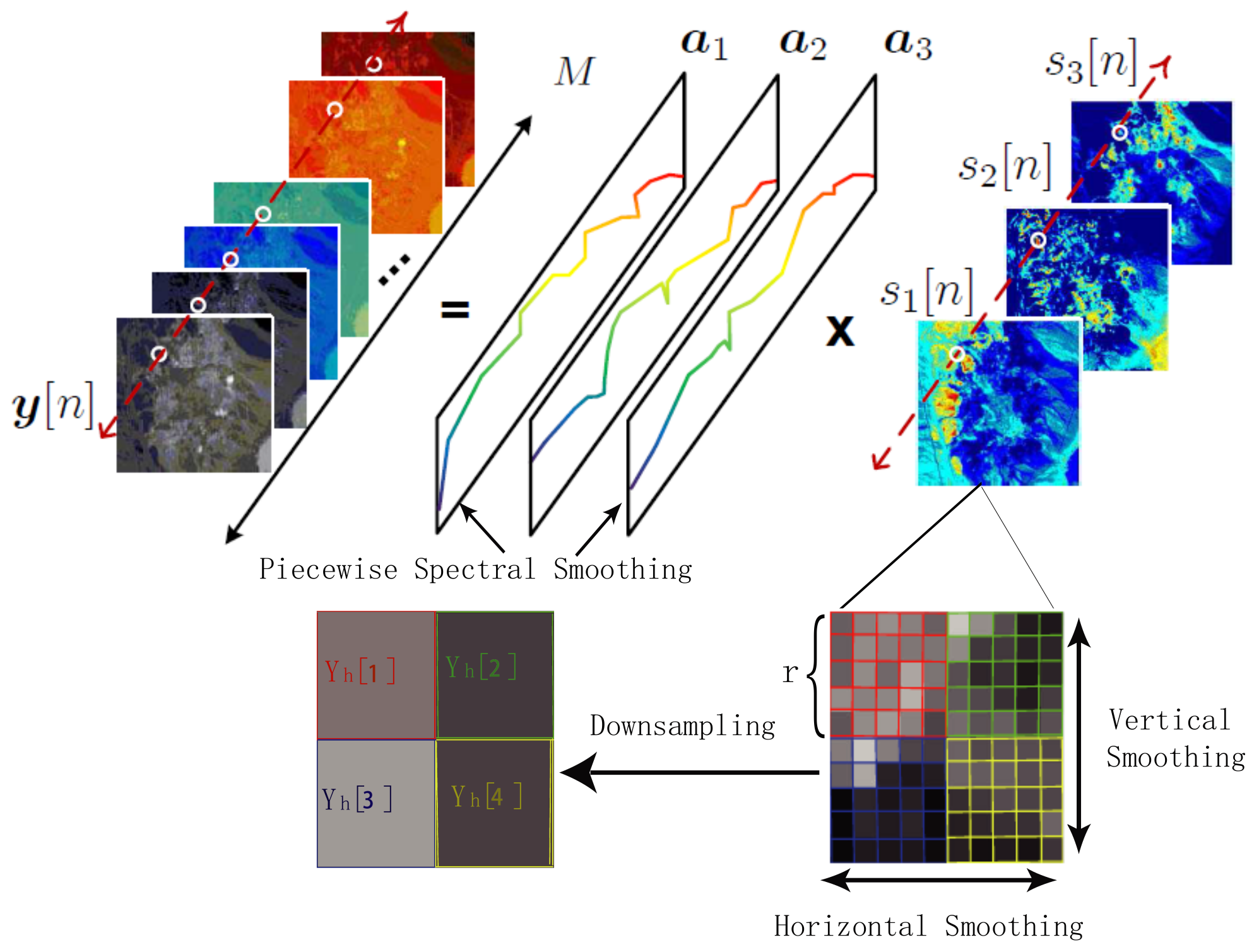
Let $\overline{\mathbf{Z}}\in {\mathbb{R}}^{W\times H\times M}$ and $\mathbf{Z}\in {\mathbb{R}}^{M\times L}$ represent the cube and matrix forms of hyperspectral data respectively, in which M is the number of spectral bands and $L=W\times H$ is the spatial resolution for each band. According to the tensor theory, the relationship of $\overline{\mathbf{Z}}$ and $\mathbf{Z}$ satisfies $\mathbf{Z}\triangleq {\overline{\mathbf{Z}}}^{\left(3\right)}$, where ${\overline{\mathbf{Z}}}^{\left(3\right)}$ denotes mode-n (i.e., $n=3$) product [18,23]. So, we can handle the data matrix $\mathbf{Z}$ in the following sessions.

2.1. Signal Models

Based on linear mixed model (LMM) shown in Figure 1, the hyperspectral data $\mathbf{Z}$ can be factorized into the product of two matrices [2], i.e.,

$$\begin{array}{c}\hfill \mathbf{Z}=\mathbf{AS},\end{array}$$

(1)

where $\mathbf{A}⪰{\mathbf{0}}_{M\times N}$ is the endmember signature matrix containing N endmembers; $\mathbf{S}⪰{\mathbf{0}}_{N\times L}$ is the abundance matrix containing the fractions of endmembers for each pixel [37]. Besides the non-negativity condition, $\mathbf{S}$ also satisfies the sum-to-one constraint $1_N^T\mathbf{S}=1_L^T$; that is, the sum of the abundance of substances in each pixel is equal to 1. However, the $L_1$-norm of $\mathbf{S}$ is equal to a constant when $\mathbf{S}$ is sparse, which makes the sum-to-one constraint unnecessary. Furthermore, according to observation model, the desired data $\mathbf{Z}$ can also be degraded respectively spatially and spectrally to yield the observed hyperspectral data ${\mathbf{Y}}_h\in {\mathbb{R}}^{M\times L_h}$ and multispectral data ${\mathbf{Y}}_m\in {\mathbb{R}}^{M_m\times L}$, where $L_h$ denotes the number of pixels in ${\mathbf{Y}}_h$ and $M_m$ represents the number of spectral bands in ${\mathbf{Y}}_m$.

Combining LMM with the observation model, we have

$$\begin{array}{cc}\hfill {\mathbf{Y}}_h& =\mathbf{Z}\mathbf{G}+{\mathbf{E}}_h=\mathbf{AS}\mathbf{G}+{\mathbf{E}}_h,\hfill \end{array}$$

(2)

$$\begin{array}{cc}\hfill {\mathbf{Y}}_m& =\mathbf{F}\mathbf{Z}+{\mathbf{E}}_m=\mathbf{F}\mathbf{AS}+{\mathbf{E}}_m,\hfill \end{array}$$

(3)

where ${\mathbf{E}}_h$ and ${\mathbf{E}}_m$ are the residuals of observed HSI and MSI data, respectively. The matrix $\mathbf{F}\in {\mathbb{R}}^{M_m\times M}$, constructed by the uniform spectral response of two observed sensors, downsamples the hyperspectral bands of $\mathbf{Z}$ to yield the multispectral data ${\mathbf{Y}}_m$. The matrix $\mathbf{G}={\mathbf{I}}_{L_h}\otimes \mathbf{g}\in {\mathbb{R}}^{L\times L_h}$, derived from a point spread function, degrades the desired data $\mathbf{Z}$ to obtain the observed hyperspectral data ${\mathbf{Y}}_h$ [25,36,38]. Using a Guassian kernel with a blurring factor of $r\triangleq \sqrt{L/L_h}$ shown in Figure 1, $\mathbf{G}$ is defined as

$$\mathbf{G}={\mathbf{I}}_{L_h}\otimes \mathbf{g}\in {\mathbb{R}}^{L\times L_h},$$

(4)

where $\mathbf{g}\in {\mathbb{R}}^{r^2}$ is a Gaussian kernel vector. In this article, $\mathbf{F}$ and $\mathbf{G}$ can be estimated from the datasets for the fusion method [25,32].

From Equations (2) and (3), the objective function of original CNMF proposed in [25] is formulated as two coupled data fidelity terms; i.e.,

$$\begin{array}{cc}\hfill \underset{\mathbf{A},\mathbf{S}}{min}& \mathbf{C}(\mathbf{A},\mathbf{S})\triangleq {\parallel {\mathbf{Y}}_h-\mathbf{A}\mathbf{S}\mathbf{G}\parallel }_F^2+{\parallel {\mathbf{Y}}_m-\mathbf{F}\mathbf{A}\mathbf{S}\parallel }_F^2\hfill \\ \hfill \mathrm{s}.\mathrm{t}.& \mathbf{A}⪰{\mathbf{0}}_{M\times N},\mathbf{S}⪰{\mathbf{0}}_{N\times L}.\hfill \end{array}$$

(5)

As an ill-posed inverse problem, the original CNMF is also susceptible to noise and the loss of data structure information caused by the matrixing method.

2.2. Problem Formulation

According to Craig’s belief, all the pixels should be enclosed in the minimum-volume simplex [24,39]. On this basis, this article imposes the regularization of joint spatial-spectral smoothing, as well as spatial sparsity, on the original CNMF to redefine the regularized fusion problem. Therefore, we get

$$\begin{array}{cc}\hfill \underset{\mathbf{A},\mathbf{S}}{min}& \frac{1}{2}\mathbf{C}(\mathbf{A},\mathbf{S})+{\lambda }_a{\varphi }_a\left(\mathbf{A}\right)+{\lambda }_e{\varphi }_e\left(\mathbf{A}\right)+{\lambda }_h{\varphi }_h\left(\mathbf{S}\right)+{\lambda }_s{\varphi }_s\left(\mathbf{S}\right)\hfill \\ \hfill \mathrm{s}.\mathrm{t}.& \mathbf{A}⪰{\mathbf{0}}_{M\times N},\mathbf{S}⪰{\mathbf{0}}_{N\times L}\hfill \end{array}$$

(6)

where ${\lambda }_a$, ${\lambda }_e$, ${\lambda }_h$ and ${\lambda }_s$ are the regularization parameters; ${\varphi }_a\left(\mathbf{A}\right)$ is the minimum-volume regularizer; ${\varphi }_e\left(\mathbf{A}\right)$ and ${\varphi }_h\left(\mathbf{S}\right)$ are the spatial and spectral smoothing regularizers, respectively; and ${\varphi }_s\left(\mathbf{S}\right)$ is to promote the sparsity of abundance matrix. These regularization expressions are defined as follows [40,41,42]:

$$\begin{array}{cc}\hfill & {\varphi }_a\left(\mathbf{A}\right)\triangleq \frac{1}{2}\sum _{j=1}^N{\parallel {\mathbf{a}}_j-{\overline{\mathbf{\mu }}}_y\parallel }_2^2,\hfill \end{array}$$

(7a)

$$\begin{array}{cc}\hfill & {\varphi }_e\left(\mathbf{A}\right)\triangleq \sum _{j=1}^N\sum _{\{m,n\}\in \gamma }|{\mathbf{a}}_j\left(m\right)-{\mathbf{a}}_j\left(n\right)|,\hfill \end{array}$$

(7b)

$$\begin{array}{cc}\hfill & {\varphi }_s\left(\mathbf{S}\right)\triangleq {\parallel \mathbf{S}\parallel }_{1,1},\hfill \end{array}$$

(7c)

$$\begin{array}{cc}\hfill & {\varphi }_h\left(\mathbf{S}\right)\triangleq \sum _{\{m,n\}\in ϵ}{\parallel {\mathbf{s}}_m-{\mathbf{s}}_n\parallel }_1,\hfill \end{array}$$

(7d)

where $ϵ$ is the set of horizontal and vertical neighbors in the image; $\gamma$ denotes the set of vertical neighbors in endmember matrix; ${\mathbf{a}}_j\left(m\right)$ is the mth component of jth endmember ${\mathbf{a}}_j$; and ${\parallel \mathbf{S}\parallel }_{1,1}={\sum }_{j=1}^L{\parallel {\mathbf{s}}_j\parallel }_1$ (${\mathbf{s}}_j$ denotes the jth column of $\mathbf{S}$ ).

2.3. Regularization Reformulation

In hyperspectral unmixing, the well-known Craig’s belief based on convex geometry is that each hyperspectral pixel should lie in the simplex spanned by the ground-truth endmembers $\{{\mathbf{a}}_1,\cdots ,{\mathbf{a}}_N\}$; i.e., containing only one underlying material. The Craig’s minimum-volume simplex covers both spectral signature of endmembers and spatial information carried by enclosed pixels (i.e., fractional abundance ). Thus, the minimum-volume belief is well-suited as a regularizer of the original CNMF to enhance hyperspectral image resolution. Because of the high computations of minimum volume, there are some expressions that have been proposed as the surrogates of minimum volume. This article focuses on the term ${\sum }_{j=1}^N{\parallel {\mathbf{a}}_j-\overline{\mathbf{\mu }}\parallel }_2^2$, which makes each column (i.e., each endmember) of $\mathbf{A}$ as close to $\overline{\mathbf{\mu }}$ as possible, as shown in Figure 2. From this figure, we can observe that $\overline{\mathbf{\mu }}$ is the geometric center of the minimum-volume simplex, i.e., $\overline{\mathbf{\mu }}=\frac{1}{N}{\sum }_{i=1}^N{\mathbf{a}}_i$, in which the red triangle is the optimal simplex and k is the number of iterations. For the convenience of calculation, ${\sum }_{j=1}^N{\parallel {\mathbf{a}}_j-\frac{1}{N}{\sum }_{i=1}^N{\mathbf{a}}_i\parallel }_2^2$ can be reformulated into the form of a matrix-vector product. Therefore, using the relationship between the jth (or ith) column ${\mathbf{a}}_j$ (or ${\mathbf{a}}_i$) and the endmember vector $\mathbf{a}\triangleq \mathbf{vec}\left(\mathbf{A}\right)$, a matrix $\mathbf{P}$ is constructed to make the equation true as

$${\varphi }_a\left(\mathbf{A}\right)=\frac{1}{2}\sum _{j=1}^N{\parallel {\mathbf{a}}_j-\frac{1}{N}\sum _{i=1}^N{\mathbf{a}}_i\parallel }_2^2=\frac{1}{2}{\parallel \mathbf{P}\mathbf{a}\parallel }_2^2,$$

(8)

where $\mathbf{P}={\mathbf{I}}_{MN}-\frac{1}{N}({\mathbf{1}}_N\otimes {\mathbf{I}}_M)$.

The endmember signature describes the spectral reflectance of a substance, which seems to be an intrinsic identity. Regardless of the bands absorbed by vapor, the spectral signature of each endmember is theoretically a smooth curve in Figure 3. It would be piecewise smooth if some bands were to be removed or absorbed by vapor. Equation (7b) aims at smoothing the signature curve, but it is in scalar form. Therefore, we establish a vertical difference matrix ${\overline{\mathbf{D}}}_e$ using a Toeplitz matrix to promote the smoothing of endmember signature, and then Equation (7b) can be converted as the vertical total variation ${\parallel {\overline{\mathbf{D}}}_e\mathbf{A}\parallel }_{1,1}$. When the matrix $\mathbf{A}$ is vectorized as $\mathbf{a}$, (7b) can be reformulated as

$${\varphi }_e\left(\mathbf{A}\right)=\sum _{j=1}^N\sum _{\{m,n\}\in \gamma }|{\mathbf{a}}_j\left(m\right)-{\mathbf{a}}_j\left(n\right)|={\parallel {\mathbf{D}}_e\mathbf{a}\parallel }_1$$

(9)

where ${\mathbf{D}}_e={\mathbf{I}}_M\otimes {\overline{\mathbf{D}}}_e$ is the vector-based difference matrix.

The regularizer that we use, ${\sum }_{\{m,n\}\in ϵ}{\parallel {\mathbf{s}}_m-{\mathbf{s}}_n\parallel }_1$, known as anisotropic total variation, is employed to promote image piecewise smoothing and further reduce the impact of structure information loss. Furthermore, anisotropy total variation can be reshaped into a vector-based form, which has two meanings: one is the vectorization of the abundance matrix for separately yielding the horizontal and vertical difference matrices, and the other is the combination of two difference matrices into a block vector. Let $\overline{\mathbf{S}}$ be a frontal slice (i.e., single-band image data) of hyperspectral data cube $\overline{\mathbf{Z}}$ with the size of $L_y\times L_x$ pixels (i.e., $L_y=L_x=\sqrt{L}$). The vertical and horizontal differences of $\overline{\mathbf{S}}$ can be presented as ${\mathbf{R}}_L\overline{\mathbf{S}}$ and $\overline{\mathbf{S}}{\mathbf{R}}_L^T$, respectively, where ${\mathbf{R}}_L$ is the first-order difference matrix [42], defined as

$${\mathbf{R}}_L(m,n)\triangleq \left\{\begin{array}{cc}1,\hfill & n=m+1,\hfill \\ -1,\hfill & n=m,\hfill \\ 0,\hfill & \mathrm{otherwise}.\hfill \end{array}\right.$$

when the spatial data $\overline{\mathbf{S}}$ is reformed as a vector via vector-matrix operator, the vertical and horizontal difference matrices are presented as ${\mathbf{D}}_v={\mathbf{I}}_L\otimes {\mathbf{R}}_L$ and ${\mathbf{D}}_h={\mathbf{R}}_L\otimes {\mathbf{I}}_L$, respectively. Then, these two difference matrices are incorporated into a block vector $\overline{\mathbf{H}}=[{\mathbf{D}}_v;{\mathbf{D}}_h]$. With due consideration of N endmembers aforementioned, the ultimate vector-based difference matrix is constructed as $\mathbf{H}=\overline{\mathbf{H}}\otimes {\mathbf{I}}_N$. The regularizer ${\sum }_{\{m,n\}\in ϵ}{\parallel {\mathbf{s}}_m-{\mathbf{s}}_n\parallel }_1$ in (7d) can be reformulated into the form of a matrix-vector product as

$${\varphi }_h\left(\mathbf{S}\right)=\sum _{\{m,n\}\in ϵ}{\parallel {\mathbf{s}}_m-{\mathbf{s}}_n\parallel }_1={\parallel \mathbf{H}\mathbf{s}\parallel }_1,$$

(10)

where $\mathbf{s}\triangleq \mathbf{vec}\left(\mathbf{S}\right)\in {\mathbb{R}}^{NL}$. In addition, the expression of ${\parallel \mathbf{S}\parallel }_{1,1}$ can be converted directly to ${\parallel \mathbf{s}\parallel }_1$.

Furthermore, One can observe that (6) is a bi-convex problem, that is, it is convex when we fix either $\mathbf{A}$ or $\mathbf{S}$ alone. Alternating optimization (AO) is widely used to solve the bi-convex problem.

3. Proposed Fusion Algorithm

In this section, we incorporate the regularization of joint spatial-spectral smoothing in a minimum volume simplex into the CNMF framework, and propose the CNMF-based fusion method (termed JSMV-CNMF) to solve the problem (6).

3.1. JSMV-CNMF Algorithm via AO

To reconstruct the high-spatial-resolution HSIs by calculating $\mathbf{A}$ and $\mathbf{S}$, the JSMV-CNMF algorithm is proposed via AO, as shown in Algorithm 1. The JSMV-CNMF iteratively updates the following two convex subproblems until convergence,

$$\begin{array}{cc}\hfill {\mathbf{S}}^{k+1}\in arg\underset{\mathbf{S}⪰{\mathbf{0}}_{N\times L}}{min}& \frac{1}{2}\mathbf{C}({\mathbf{A}}^k,\mathbf{S})+{\lambda }_h{\varphi }_h\left(\mathbf{S}\right)+{\lambda }_s{\varphi }_s\left(\mathbf{S}\right),\hfill \end{array}$$

(11)

$$\begin{array}{cc}\hfill {\mathbf{A}}^{k+1}\in arg\underset{\mathbf{A}⪰{\mathbf{0}}_{M\times N}}{min}& \frac{1}{2}\mathbf{C}(\mathbf{A},{\mathbf{S}}^k)+{\lambda }_a{\varphi }_a\left(\mathbf{A}\right)+{\lambda }_e{\varphi }_e\left(\mathbf{A}\right),\hfill \end{array}$$

(12)

where k is the iteration number of the outer loop. Owing to the iterative order of S prior to A, an initial value of ${\mathbf{A}}^0$ can be determined by successive projection algorithm [43,44]. To solve these subproblems (11) and (12), the alternating direction method of multipliers (ADMM) [45] is utilized to design an efficient solver in the following subsections.

Algorithm 1 JSMV-CNMF algorithm for solving (6).

1: Input: ${\mathbf{Y}}_h$, ${\mathbf{Y}}_m$, $\mathbf{F}$ and $\mathbf{G}$. 2: Output $\mathbf{Z}={\mathbf{A}}^k{\mathbf{S}}^k$. 3: Initialize ${\mathbf{A}}^0$. 4: $k=0$. 5: while the stopping rule of the outer loop is not met do 6:  update ${\mathbf{S}}^{k+1}$ by (11); 7:  update ${\mathbf{A}}^{k+1}$ by (12); 8:  $k:=k+1$; 9: end while.

3.2. Abundance Estimation via ADMM

Using ADMM and Kronecker operators, we can integrate two Frobenius-norm terms into an ${\ell }_2$-norm term by vectorizing the variable $\mathbf{S}$. In (11), the bottleneck lies in the heavy complexities of ${\mathbf{B}}_1$ and $\mathbf{H}$. By splitting the primal variables into several separable components via equality constraints, we rewrite (11) as

$$\begin{array}{cc}\hfill \underset{\mathbf{s},\mathbf{u},\mathbf{v},\mathbf{x}}{min}& \frac{1}{2}{\parallel {\mathbf{B}}_1\mathbf{s}-\mathbf{y}\parallel }_2^2+{\lambda }_h{\parallel \mathbf{v}\parallel }_1+{\lambda }_s{\parallel \mathbf{x}\parallel }_1+I_{+}\left(\mathbf{x}\right)\hfill \\ \hfill \mathrm{s}.\mathrm{t}.& \mathbf{s}=\mathbf{u},\hfill \\ \hfill & \mathbf{v}=\mathbf{H}\mathbf{u},\hfill \\ \hfill & \mathbf{s}=\mathbf{x},\hfill \end{array}$$

(13)

where ${\mathbf{B}}_1\triangleq {[{({\mathbf{G}}^T\otimes {\mathbf{A}}^k)}^T,{({\mathbf{I}}_L\otimes \mathbf{F}{\mathbf{A}}^k)}^T]}^T\in {\mathbb{R}}^{(M{L}_h+L{M}_m)\times NL}$; $\mathbf{y}\triangleq {[\mathbf{vec}{\left({\mathbf{Y}}_h\right)}^T,\mathbf{vec}{\left({\mathbf{Y}}_m\right)}^T]}^T\in {\mathbb{R}}^{M{L}_h+L{M}_m}$; and $I_{+}\left(\mathbf{x}\right)$ is a indicator function, defined as

$$I_{+}\left(\mathbf{x}\right)\triangleq \left\{\begin{array}{cc}0,\hfill & \mathrm{if}\mathbf{x}⪰{\mathbf{0}}_{MN},\hfill \\ \infty ,\hfill & \mathrm{otherwise}.\hfill \end{array}\right.$$

In addition, the equation constraint $\mathbf{s}=\mathbf{u}$ is introduced to separate the $\mathbf{s}$ and $\mathbf{v}$ using the variable $\mathbf{u}$ for reducing the complexity of closed-form solutions. Then, we can obtain the augmented Lagrangian of (13) by

$$\begin{array}{cc}\hfill \mathcal{L}(\mathbf{s},\mathbf{u},\mathbf{v},\mathbf{x},{\mathbf{h}}_i)=& \frac{1}{2}{\parallel {\mathbf{B}}_1\mathbf{s}-\mathbf{y}\parallel }_2^2+{\lambda }_h{\parallel \mathbf{v}\parallel }_1+{\lambda }_s{\parallel \mathbf{x}\parallel }_1+I_{+}\left(\mathbf{x}\right)+{{\mathbf{h}}_1}^T(\mathbf{s}-\mathbf{u})+{\displaystyle \frac{\eta }{2}}{\parallel \mathbf{s}-\mathbf{u}\parallel }_2^2\hfill \\ \hfill & +{{\mathbf{h}}_2}^T(\mathbf{v}-\mathbf{H}\mathbf{u})+{\displaystyle \frac{\eta }{2}}{\parallel \mathbf{v}-\mathbf{H}\mathbf{u}\parallel }_2^2+{{\mathbf{h}}_3}^T(\mathbf{s}-\mathbf{x})+{\displaystyle \frac{\eta }{2}}{\parallel \mathbf{s}-\mathbf{x}\parallel }_2^2,\hfill \end{array}$$

(14)

where ${\mathbf{h}}_i(i=1,\cdots ,3)$ are called dual variables, and $\eta$ is the weight. Via ADMM, these primal and dual variables can be iteratively updated in step with provable convergence [46] by

$$\begin{array}{cc}\hfill {\mathbf{s}}^{j+1}& \in arg\underset{\mathbf{s}\in {\mathbb{R}}^{NL}}{min}\mathcal{L}(\mathbf{s},{\mathbf{u}}^j,{\mathbf{x}}^j,{{\mathbf{h}}_1}^j,{{\mathbf{h}}_3}^j),\hfill \end{array}$$

(15a)

$$\begin{array}{cc}\hfill {\mathbf{u}}^{j+1}& \in arg\underset{\mathbf{u}\in {\mathbb{R}}^{NL}}{min}\mathcal{L}({\mathbf{s}}^{j+1},\mathbf{u},{\mathbf{v}}^j,{{\mathbf{h}}_1}^j,{{\mathbf{h}}_2}^j),\hfill \end{array}$$

(15b)

$$\begin{array}{cc}\hfill {\mathbf{v}}^{j+1}& \in arg\underset{\mathbf{v}\in {\mathbb{R}}^{2N\sqrt{L}(\sqrt{L}-1)}}{min}\mathcal{L}({\mathbf{u}}^{j+1},\mathbf{v},{{\mathbf{h}}_2}^j),\hfill \end{array}$$

(15c)

$$\begin{array}{cc}\hfill {\mathbf{x}}^{j+1}& \in arg\underset{\mathbf{x}\in {\mathbb{R}}_{+}^{NL}}{min}\mathcal{L}({\mathbf{s}}^{j+1},\mathbf{x},{{\mathbf{h}}_3}^j),\hfill \end{array}$$

(15d)

$$\begin{array}{cc}\hfill {{\mathbf{h}}_1}^{j+1}& ={{\mathbf{h}}_1}^j+\eta ({\mathbf{s}}^{j+1}-{\mathbf{u}}^{j+1}),\hfill \end{array}$$

(15e)

$$\begin{array}{cc}\hfill {{\mathbf{h}}_2}^{j+1}& ={{\mathbf{h}}_2}^j+\eta ({\mathbf{v}}^{j+1}-\mathbf{H}{\mathbf{u}}^{j+1}),\hfill \end{array}$$

(15f)

$$\begin{array}{cc}\hfill {{\mathbf{h}}_3}^{j+1}& ={{\mathbf{h}}_3}^j+\eta ({\mathbf{s}}^{j+1}-{\mathbf{x}}^{j+1}),\hfill \end{array}$$

(15g)

where j denotes the iteration number of inner loop. Combined with the expression (14), subproblems (15a) ⋯ (15d) can easily converted into the scaled forms as

$$\begin{array}{cc}\hfill {\mathbf{s}}^{j+1}& \in arg\underset{\mathbf{s}\in {\mathbb{R}}^{NL}}{min}\frac{1}{2}{\parallel {\mathbf{B}}_1\mathbf{s}-\mathbf{y}\parallel }_2^2+{\displaystyle \frac{\eta }{2}}{\parallel \mathbf{s}-{\mathbf{u}}^j+{\widetilde{{\mathbf{h}}_1}}^j\parallel }_2^2+{\displaystyle \frac{\eta }{2}}{\parallel \mathbf{s}-{\mathbf{x}}^j+{\widetilde{{\mathbf{h}}_3}}^j\parallel }_2^2,\hfill \end{array}$$

(16a)

$$\begin{array}{cc}\hfill {\mathbf{u}}^{j+1}& \in arg\underset{\mathbf{u}\in {\mathbb{R}}^{NL}}{min}{\displaystyle \frac{\eta }{2}}{\parallel {\mathbf{s}}^{j+1}-\mathbf{u}+{\widetilde{{\mathbf{h}}_1}}^j\parallel }_2^2+{\displaystyle \frac{\eta }{2}}{\parallel {\mathbf{v}}^j-{\mathbf{D}}_v\mathbf{u}+{\widetilde{{\mathbf{h}}_2}}^j\parallel }_2^2,\hfill \end{array}$$

(16b)

$$\begin{array}{cc}\hfill {\mathbf{v}}^{j+1}& \in arg\underset{\mathbf{v}\in {\mathbb{R}}^{2N\sqrt{L}(\sqrt{L}-1)}}{min}{\lambda }_h{\parallel \mathbf{v}\parallel }_1+{\displaystyle \frac{\eta }{2}}{\parallel \mathbf{v}-\mathbf{H}{\mathbf{u}}^{j+1}+{\widetilde{{\mathbf{h}}_2}}^j\parallel }_2^2,\hfill \end{array}$$

(16c)

$$\begin{array}{cc}\hfill {\mathbf{x}}^{j+1}& \in arg\underset{\mathbf{x}\in {\mathbb{R}}_{+}^{NL}}{min}{\lambda }_s{\parallel \mathbf{x}\parallel }_1+{\displaystyle \frac{\eta }{2}}{\parallel {\mathbf{s}}^{j+1}-\mathbf{x}+{\widetilde{{\mathbf{h}}_3}}^j\parallel }_2^2,\hfill \end{array}$$

(16d)

where $\widetilde{{\mathbf{h}}_i}\triangleq {\mathbf{h}}_i/\eta ,(i=1,2,3)$ are the scaled dual variables. Since $\mathbf{s}$ is the first iteration variable, the initial values of other variables can be assigned to zeros or warm start [45], including ${\mathbf{u}}^0$, ${\mathbf{x}}^0$, ${\mathbf{v}}^0$ and ${\widetilde{{\mathbf{h}}_i}}^0$.

We can observe that (16a) and (16b) are both unconstrained quadratic problems; (16c) is a generalized Lasso problem [45]; and (16d) can be solved by KKT optimal condition [32,42], and then projected to a non-negative orthant ${\mathcal{R}}_{+}^{NL}$. Thus, we can obtain the closed-form solutions as

$$\begin{array}{cc}\hfill {\mathbf{s}}^{j+1}=& {({\mathbf{B}}_1^T{\mathbf{B}}_1+2\eta {\mathbf{I}}_{NL})}^{-1}({\mathbf{B}}_1^T\mathbf{y}+\eta {\mathbf{u}}^j-{{\mathbf{h}}_1}^j+\eta {\mathbf{x}}^j-{{\mathbf{h}}_3}^j),\hfill \end{array}$$

(17a)

$$\begin{array}{cc}\hfill {\mathbf{u}}^{j+1}=& {({\mathbf{H}}^T\mathbf{H}+{\mathbf{I}}_{NL})}^{-1}[{\mathbf{H}}^T({\mathbf{v}}^j+{\widetilde{{\mathbf{h}}_2}}^j)+{\mathbf{s}}^{j+1}+{\widetilde{{\mathbf{h}}_1}}^j],\hfill \end{array}$$

(17b)

$$\begin{array}{cc}\hfill {\mathbf{v}}^{j+1}=& \mathrm{shrink}(\mathbf{H}{\mathbf{u}}^{j+1}-{\widetilde{{\mathbf{h}}_2}}^j,{\lambda }_h/\eta ),\hfill \end{array}$$

(17c)

$$\begin{array}{cc}\hfill {\mathbf{x}}^{j+1}=& {\left[{\mathbf{s}}^{j+1}+{\widetilde{{\mathbf{h}}_3}}^j-({\lambda }_s/\eta ){\mathbf{1}}_{NL}\right]}_{+},\hfill \end{array}$$

(17d)

where $\mathrm{shrink}(\mathbf{s},\gamma )=\mathrm{sgn}\left(\mathbf{s}\right)\max (\left|\mathbf{s}\right|-\gamma ,0).$ The computation of (17a) is $\mathcal{O}\left(L_h{\left(NL\right)}^2\xi \right)$, where $\xi \triangleq max\{M,M_m{r}^2,N{r}^2\}$. It is obvious that the computation of ${\mathbf{B}}_1^T{\mathbf{B}}_1$ is the bottleneck when the value of L is large. To decrease the computation burden, we define ${\overline{\mathbf{B}}}_1\triangleq {[{({\mathbf{g}}^T\otimes {\mathbf{A}}^k)}^T,{({\mathbf{I}}_{r^2}\otimes \mathbf{F}{\mathbf{A}}^k)}^T]}^T\in {\mathbb{R}}^{(M+r^2{M}_m)\times N{r}^2}$, ${\mathbf{B}}_1^T\mathbf{y}\triangleq \mathbf{vec}\left({({\mathbf{g}}^T\otimes {\mathbf{A}}^k)}^T{\mathbf{Y}}_h\right)+\mathbf{vec}\left({\left({\mathbf{FA}}^k\right)}^T{\mathbf{Y}}_m\right)$ and $\tilde{\mathbf{v}}\triangleq {\mathbf{B}}_1^T\mathbf{y}+\eta {\mathbf{u}}^j-{\mathbf{h}}_1^j+{\mathbf{x}}^j-{\mathbf{h}}_3^j)$, and then convert $\tilde{\mathbf{v}}$ into a matrix $\tilde{\mathbf{V}}\in {\mathcal{R}}^{N{r}^2\times L_h}$. Using structure matrix (4) and Kronecker operators, the optimized solution of (17a) is rewritten [32] as

$$\begin{array}{c}\hfill {\mathbf{s}}^{j+1}=\mathbf{vec}\left({({\overline{\mathbf{B}}}_1^T{\overline{\mathbf{B}}}_1+2\eta {\mathbf{I}}_{N{r}^2})}^{-1}\tilde{\mathbf{V}}\right),\end{array}$$

(18)

whose computation takes the complexity of $\mathcal{O}\left(({\left(N{r}^2\right)}^2+NL)\xi \right)$, much lower than that of (17a).

In the same way, to reduce the high complexity of $\mathcal{O}\left({\left(NL\right)}^3\right)$ in (17b), we define ${\tilde{\mathbf{u}}}_1\triangleq {\mathbf{v}}_1^j+{\widetilde{{\mathbf{h}}_2}}^j$ and ${\tilde{\mathbf{u}}}_2\triangleq {\mathbf{s}}^{j+1}+{\widetilde{{\mathbf{h}}_1}}^j$, and then reshape these two vectors into the matrices ${\tilde{\mathbf{U}}}_1$ and ${\tilde{\mathbf{U}}}_2$, respectively. By the structure of difference matrix $\mathbf{H}$, (17b) is simplified as

$$\begin{array}{cc}\hfill {\mathbf{u}}^{j+1}& =\mathbf{vec}\left(\{\left[{({\overline{\mathbf{R}}}_{L_y}^T{\overline{\mathbf{R}}}_{L_y}+\eta {\mathbf{I}}_{L_y})}^{-1}{\overline{\mathbf{R}}}_{L_y}^T\right]\otimes {\mathbf{I}}_N\}{\tilde{\mathbf{U}}}_1\right)+\mathbf{vec}\left([{({\overline{\mathbf{R}}}_{L_y}^T{\overline{\mathbf{R}}}_{L_y}+\eta {\mathbf{I}}_{L_y})}^{-1}\otimes {\mathbf{I}}_N]{\tilde{\mathbf{U}}}_2\right),\hfill \end{array}$$

(19)

which involves the computation of $\mathcal{O}\left(N^{2}L\sqrt{L}\right)$, much less than (17b). In summary, in order to obtain the abundance matrix $\mathbf{S}$ by alternatively iterating the above original and dual variables, the resulting ADMM-based algorithm for solving (11) is presented in Algorithm 2.

Algorithm 2 Solving (11) via ADMM

1: Input: N, ${\mathbf{Y}}_h$, ${\mathbf{Y}}_m$, $\mathbf{F}$, $\mathbf{G}$ and ${\mathbf{A}}^k$. 2: Output ${\mathbf{S}}^{k+1}$. 3: Initialize ${\mathbf{u}}^0$, ${\mathbf{z}}^0$, ${\mathbf{x}}^0$,${\mathbf{v}}^0$ and ${\mathbf{h}}_i^0(i=1,\cdots ,3)$ with $\mathbf{0}$ or warm start. 4: $j=0$ 5: while the predefined stopping rule of the inner loop is not met do 6:  update ${\mathbf{s}}^{j+1}$ by (18); 7:  update ${\mathbf{u}}^{j+1}$ by (19); 8:  update ${\mathbf{v}}^{j+1}$ by (17c); 9:  update ${\mathbf{x}}^{j+1}$ by (17d); 10:  update ${\widetilde{{\mathbf{h}}_i}}^{j+1}={{\mathbf{h}}_i}^{j+1}/\eta$ ($i=1,2,3$) by (15e) ⋯ (15g), respectively; 11:  $j:=j+1$; 12: end while.

3.3. Endmember Estimation via ADMM

Similar to the above process of abundance estimation, we reformulate (12) in such a vector-based form that the primal variable can also be divided into several separable elements with equality constraints. To be exact, we rewrite (12) as

$$\begin{array}{cc}\hfill \underset{\mathbf{a},\mathbf{b},\mathbf{w},\mathbf{d}}{min}& {\displaystyle \frac{1}{2}}{\parallel {\mathbf{B}}_2\mathbf{a}-\mathbf{y}\parallel }_2^2+\frac{{\lambda }_a}{2}{\parallel \mathbf{P}\mathbf{a}\parallel }_2^2+{\lambda }_e{\parallel \mathbf{w}\parallel }_1+I_{+}\left(\mathbf{d}\right)\hfill \\ \hfill \mathrm{s}.\mathrm{t}.& \mathbf{a}=\mathbf{b}\hfill \\ \hfill & \mathbf{w}={\mathbf{D}}_e\mathbf{b}\hfill \\ \hfill & \mathbf{a}=\mathbf{d}\hfill \end{array}$$

(20)

where ${\mathbf{B}}_2\triangleq {[{({\left({\mathbf{S}}^{k+1}\mathbf{G}\right)}^T\otimes {\mathbf{I}}_M)}^T,{({\left({\mathbf{S}}^{k+1}\right)}^T\otimes \mathbf{F})}^T]}^T\in {\mathbb{R}}^{(M{L}_h+L{M}_m)\times MN}$ and $\mathbf{a}=\mathbf{vec}\left(\mathbf{A}\right)\in {\mathbb{R}}_{+}^{MN}$. After splitting the variables based on the augmented Lagrangian function, we can derive the closed-form solutions as

$$\begin{array}{cc}\hfill {\mathbf{a}}^{j+1}=& {({\mathbf{B}}_2^T{\mathbf{B}}_2+{\lambda }_a{\mathbf{P}}^T\mathbf{P}+2\eta {\mathbf{I}}_{MN})}^{-1}({\mathbf{B}}_2^T\mathbf{y}+\eta {\mathbf{b}}^j-{\mathbf{f}}_1^j+\eta {\mathbf{d}}^j-{\mathbf{f}}_3^j),\hfill \end{array}$$

(21a)

$$\begin{array}{cc}\hfill {\mathbf{b}}^{j+1}=& {({\mathbf{D}}_e^T{\mathbf{D}}_e+{\mathbf{I}}_{MN})}^{-1}[{\mathbf{D}}_e^T({\mathbf{w}}^j+{{\mathbf{f}}_2}^j)+{\mathbf{a}}^{j+1}+{{\mathbf{f}}_1}^j],\hfill \end{array}$$

(21b)

$$\begin{array}{cc}\hfill {\mathbf{w}}^{j+1}=& \mathrm{shrink}({\mathbf{D}}_e{\mathbf{b}}^{j+1}-{{\mathbf{f}}_2}^j/\eta ,{\lambda }_e/\eta ),\hfill \end{array}$$

(21c)

$$\begin{array}{cc}\hfill {\mathbf{d}}^{j+1}=& {\left[{\mathbf{a}}^{j+1}+{\mathbf{f}}_1^j/\eta \right]}_{+},\hfill \end{array}$$

(21d)

$$\begin{array}{cc}\hfill {\mathbf{f}}_1^{j+1}=& {\mathbf{f}}_1^j+\eta ({\mathbf{a}}^{j+1}-{\mathbf{b}}^{j+1}),\hfill \end{array}$$

(21e)

$$\begin{array}{cc}\hfill {\mathbf{f}}_2^{j+1}=& {\mathbf{f}}_2^j+\eta ({\mathbf{w}}^{j+1}-{\mathbf{D}}_e{\mathbf{b}}^{j+1}),\hfill \end{array}$$

(21f)

$$\begin{array}{cc}\hfill {\mathbf{f}}_3^{j+1}=& {\mathbf{f}}_3^j+\eta ({\mathbf{a}}^{j+1}-{\mathbf{d}}^{j+1}).\hfill \end{array}$$

(21g)

It is not difficult to find that (21a) is time-consuming with the computational complexity of $\mathcal{O}(N^4{M}^3+{\left(NM\right)}^2{\xi }^{\prime })$, where ${\xi }^{\prime }\triangleq max\{M{L}_h,M_{m}L\}$. Thus, using the structure of ${\mathbf{B}}_2$, (21a) can be simplified [32] as

$$\begin{array}{cc}\hfill {\mathbf{a}}^{j+1}=& {\{\left(\left({\mathbf{S}}^{k+1}\mathbf{G}\right){\left({\mathbf{S}}^{k+1}\mathbf{G}\right)}^T\right)\otimes {\mathbf{I}}_M+{\lambda }_a{\mathbf{P}}^T\mathbf{P}+2\eta {\mathbf{I}}_{MN}+\left({\mathbf{S}}^{k+1}{\left({\mathbf{S}}^{k+1}\right)}^T\right)\otimes {\mathbf{F}}^T\mathbf{F}\}}^{-1}\hfill \\ \hfill & ({\mathbf{B}}_2^T\mathbf{y}+\eta {\mathbf{b}}^j-{\mathbf{f}}_1^j+\eta {\mathbf{d}}^j-{\mathbf{f}}_3^j),\hfill \end{array}$$

(22)

where ${\mathbf{B}}_2^T\mathbf{y}=\mathbf{vec}\left({\mathbf{Y}}_h{\left({\mathbf{S}}^{k+1}\mathbf{G}\right)}^T\right)+\mathbf{vec}\left({\mathbf{F}}^T{\mathbf{Y}}_m{\left({\mathbf{S}}^{k+1}\right)}^T\right)$. The computational complexity of (22) is computed by $\mathcal{O}\left(N^4{M}^3+N^{2}L\right)$, which is much lower than that of (21a). By the equation ${\mathbf{D}}_e={\mathbf{I}}_N\otimes {\overline{\mathbf{D}}}_e$, (21b) can conveniently simplified as

$$\begin{array}{cc}\hfill {\mathbf{b}}^{j+1}& =\mathbf{vec}\left({({\overline{\mathbf{D}}}_e^T{\overline{\mathbf{D}}}_e+\eta {\mathbf{I}}_M)}^{-1}{\overline{\mathbf{D}}}_e^T{\mathbf{Q}}_1\right)+\mathbf{vec}\left({({\overline{\mathbf{D}}}_e^T{\overline{\mathbf{D}}}_e+\eta {\mathbf{I}}_M)}^{-1}{\mathbf{Q}}_2\right),\hfill \end{array}$$

(23)

Put simply, aiming at the endmember matrix $\mathbf{A}$, the ADMM-based algorithm for solving (12) is given in Algorithm 3.

Algorithm 3 Solving (12) via ADMM

1: Input: N, ${\mathbf{Y}}_h$, ${\mathbf{Y}}_m$, $\mathbf{F}$, $\mathbf{G}$, and ${\mathbf{S}}^{k+1}$. 2: Output ${\mathbf{A}}^{k+1}$. 3: Initialize ${\mathbf{b}}^0$,${\mathbf{w}}^0$,${\mathbf{d}}^0$ and ${\mathbf{f}}_i^0$ ($i=1,2,3$) with ${\mathbf{0}}_{MN}$ or warm start. 4: $j=0$ 5: while the predefined stopping rule of the inner loop is not met do 6:  update ${\mathbf{a}}^{j+1}$ by (22); 7:  update ${\mathbf{b}}^{j+1}$ by (23); 8:  update ${\mathbf{w}}^{j+1}$ by (21c); 9:  update ${\mathbf{d}}^{j+1}$ by (21d); 10:  update ${\mathbf{f}}_i^{j+1}$ by (21e)–(21g), respectively; 11:  $j:=j+1$; 12: end while.

4. Experiments and Performance Analysis

In this section, the careful design of some experimental tests is described to estimate the performance of the proposed JSMV-CNMF algorithm.

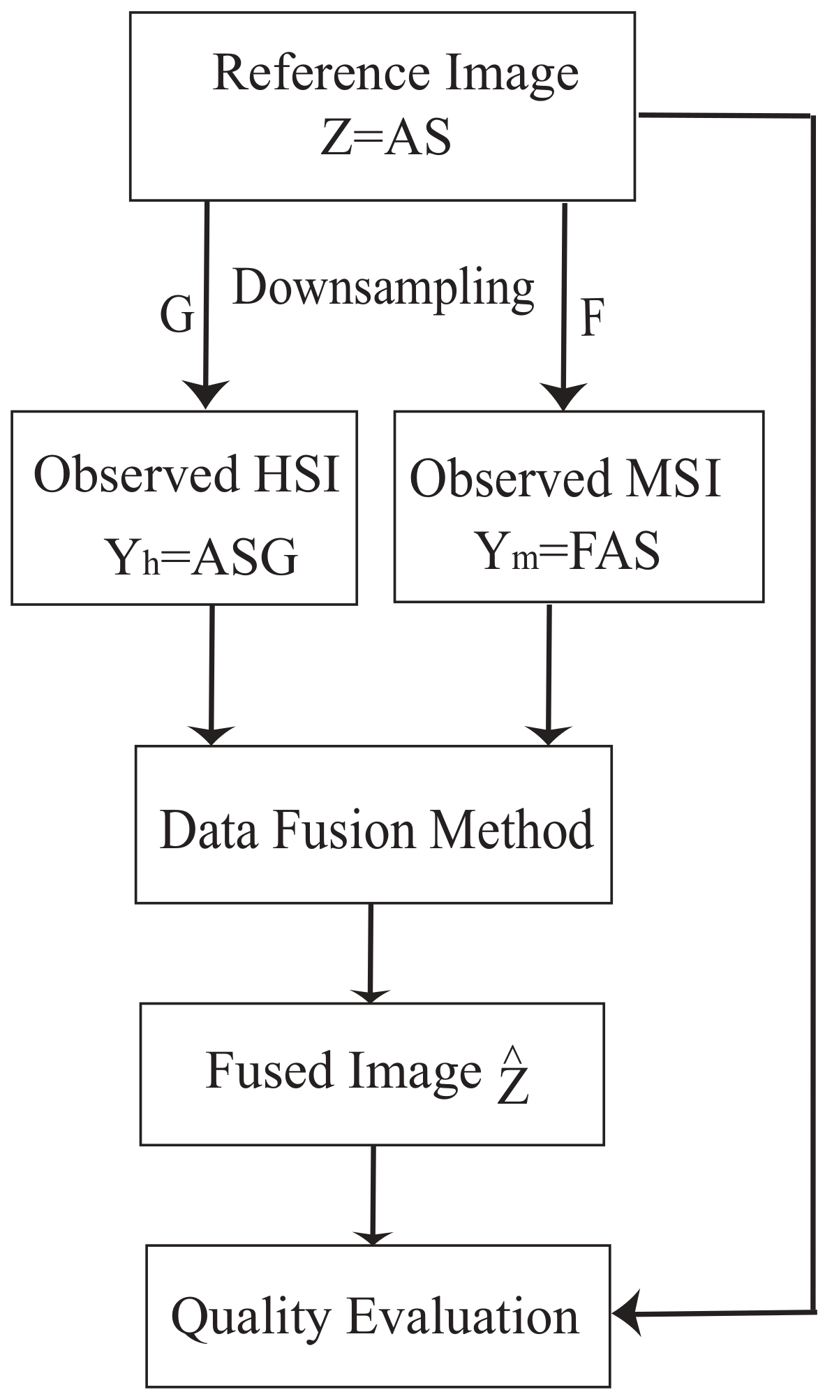
4.1. Experimental Methodology

Generally speaking, Wald’s protocol is widely used for quality assessment of fused images [5,25,47], in which the real dataset is thought of as the reference image $\mathbf{Z}$. According to the Guassian observed model, the observed HSI ${\mathbf{Y}}_h$ and MSI ${\mathbf{Y}}_m$, can be obtained by spatial and spectral degradation of high-resolution image $\mathbf{Z}$, respectively. As shown in Figure 4, the fusion method is designed to simulate the degraded images ${\mathbf{Y}}_h$ and ${\mathbf{Y}}_m$ for the fused image $\widehat{\mathbf{Z}}$. This flowchart can solve two difficulties in image fusion, including the registration of observed images and the acquisition of the ground truth for performance evaluation.

For comparison, four state-of-the-art methods were taken as the baseline, including the original CNMF [25], BSR [16], HySure [15] and tensor-based CSTF [20]. To drop the effect of randomness, the performances in the experiments were the means of multiple measurements. All the methods were tested on a laptop equipped with Intel CPU Core-3210 with 2.5 GHz speed and 16 GB RAM, using Mathworks Matlab R2015a.

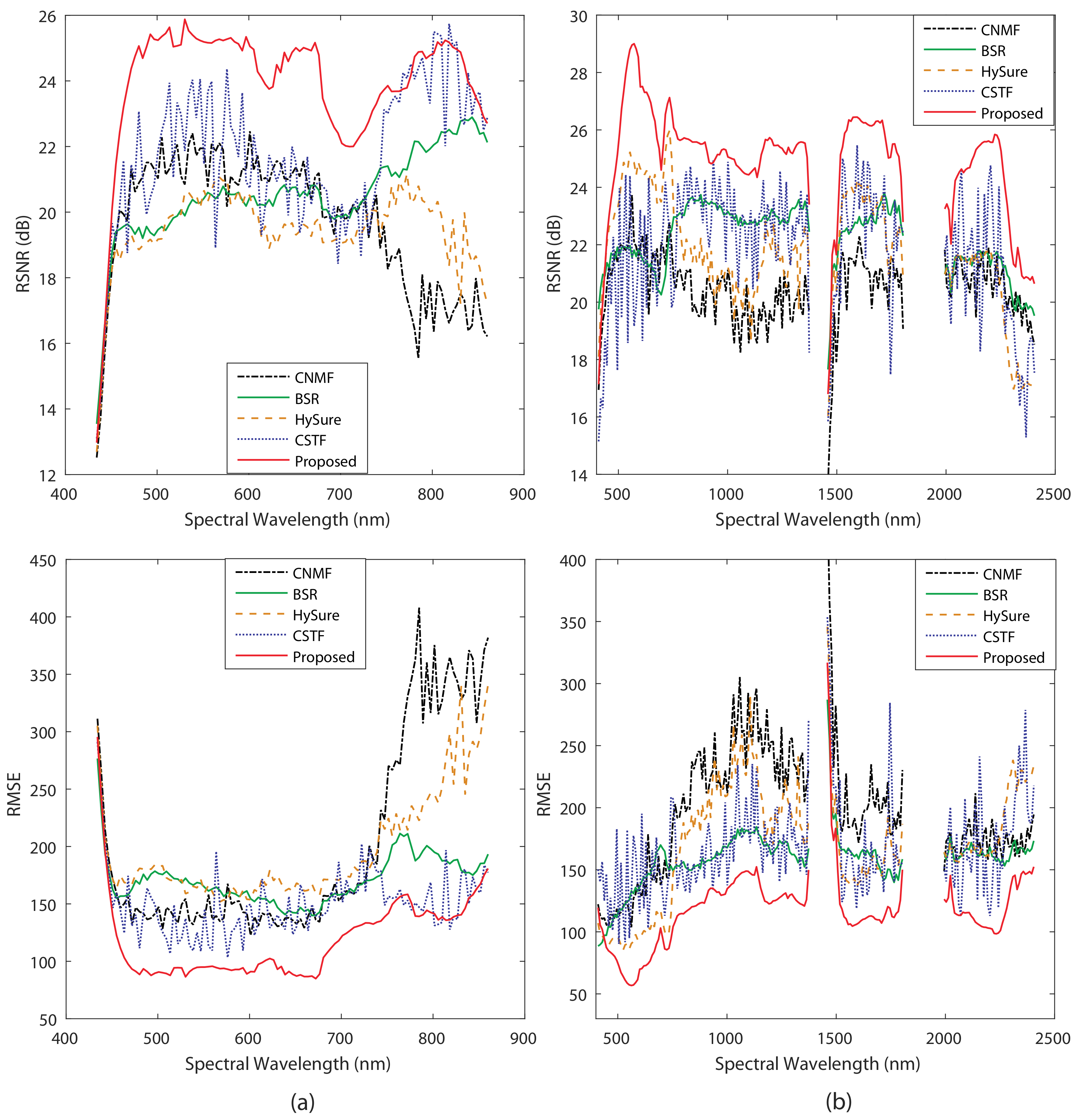
4.2. Performance Metrics

In order to quantitatively estimate the similarity between $\widehat{\mathbf{Z}}$ and $\mathbf{Z}$, some widely used performance metrics were adopted [5,16,25,32], including reconstruction signal-to-noise ratio (RSNR), root mean squared error (RMSE), spectral angle mapper (SAM), erreur relative globale adimensionnelle de synth$\stackrel{‘}{e}$se (ERGAS), degree of distortion (DD) and structural similarity index for measuring image quality (SSIM), as listed below.

• RSNR evaluates the spatial quality, defined as

  $$\mathrm{RSNR}=10{log}_{10}\left(\frac{{∥\mathbf{Z}∥}_F^2}{\parallel \widehat{\mathbf{Z}}{-\mathbf{Z}\parallel }_F^2}\right).$$
• RMSE evaluates the error of global quality by

  $$\mathrm{RMSE}=\sqrt{\frac{1}{ML}{\parallel \widehat{\mathbf{Z}}-\mathbf{Z}\parallel }_F^2}.$$

  (24)
• SAM evaluates the spectral distortion, defined as

  $$\begin{array}{c}\hfill \mathrm{SAM}=\frac{1}{L}\sum _{n=1}^L\arccos \left(\frac{{\left(\widehat{\mathbf{z}}\left[n\right]\right)}^T\mathbf{z}\left[n\right]}{\parallel \widehat{\mathbf{z}}{\left[n\right]\parallel }_2·{\parallel \mathbf{z}\left[n\right]\parallel }_2}\right)\end{array}$$

  where $\widehat{\mathbf{z}}\left[n\right]$ denotes the nth column of $\widehat{\mathbf{Z}}$.
• ERGAS evaluates the relative dimensionless global error, defined as

  $$\mathrm{ERGAS}=\frac{100}{r}\sqrt{\frac{1}{M}{\sum }_{m=1}^M\frac{{\mathrm{RMSE}}_m^2}{{\mu }_{{\mathbf{Z}}^{\left(m\right)}}^2}},$$

  where r is the blurring factor, ${\mu }_{{\mathbf{Z}}^{\left(m\right)}}$ is the mean of the mth row vector ${\mathbf{Z}}^{\left(m\right)}$ and ${\mathrm{RMSE}}_m$ is the RMSE of the mth band image.
• DD is an indicator to estimate the spectral quality, defined as

  $$\mathrm{DD}=\frac{1}{ML}{\parallel \mathrm{vec}\left(\widehat{\mathbf{Z}}\right)-\mathrm{vec}\left(\mathbf{Z}\right)\parallel }_1^2.$$
• SSIM is to measure the structure similarity between the reconstructed and reference images, defined in [48].

Generally, the higher the value of RSNR and SSIM, the better the evaluated performance. However, the lower the values of DD, RMSE, SAM and ERGAS, the less distortion. Besides theoretical complexity in order of magnitude (OM), the running time T (in seconds) is regarded as the metric of computational complexity for the fusion methods, while per-iteration running time (PRT, in seconds) is to evaluate a single time complexity of a simplified solution.

4.3. Datasets

In this study, we took two widely-used datasets acquired separately by different hyperspectral sensors to test the performance of fusion methods. The first dataset was collected over the area of Pavia University, northern Italy [49], by the reflective optics system imaging spectrometer (ROSIS) sensor, with a total of 103 spectral bands from 430 to 860 nm (corresponding to Landsat TM bands 1–4). The second dataset was captured by an airborne visible/infrared imaging spectrometer (AVIRIS) sensor over Moffett Field [50], CA, with which a total of 183 bands (ranging from 400 to 2500 nm) approximate to the Landsat TM bands 1–5 and 7. Therefore, we can separately construct the spectral response transform matrices ${\mathbf{F}}_1\in {\mathbb{R}}^{4\times 103}$ and ${\mathbf{F}}_2\in {\mathbb{R}}^{6\times 183}$, which spectrally degrade the reference data $\mathbf{Z}$ to generate their respective observed MSI data ${\mathbf{Y}}_m$ [16,25,32,36]. Furthermore, we selected the sub-scene of size $L=160\times 160$ as the target region for each dataset [16,32,36], as shown in the top row of Figure 5. With a Gaussian kernel of size $r=5$ and variance 2 [25,51], we were able to establish the matrix $\mathbf{G}\in {\mathbb{R}}^{25600\times 1024}$, which spatially degrades the reference data $\mathbf{Z}$ to obtain the observed HSI data ${\mathbf{Y}}_h$ with the size of $L_h=32\times 32$ pixels [38,52,53], which are depicted in the bottom row of Figure 5.

4.4. Parameter Settings

This article focuses on joint spatial-spectral smoothing in a minimum-volume simplex for hyperspectral image super-resolution, which is performed by incorporating four regularizers with the corresponding weights into the original CNMF method. The parameters, including ${\lambda }_a$, ${\lambda }_e$, ${\lambda }_h$ and ${\lambda }_s$ are to balance data fidelity terms and regularizers [32,51], which are relevant to the noise powers of HSIs and MSIs. For simplicity, all the weights in this article were set to the same value 0.001, i.e., ${\lambda }_a={\lambda }_e={\lambda }_h={\lambda }_s=0.001$, although the settings of these parameters deserve further study. The convergence of the proposed algorithm can be guaranteed by the threshold value and the iteration number of inner and outer loops. The stopping rule of the outer loop is that the relative difference threshold value between the successive updates of the objective function ${\mathbf{F}}_0(\mathbf{A},\mathbf{S})$ is set to $0.001$ [51]; that is,

$$\frac{{\mathbf{F}}_0({\mathbf{A}}^{k+1},{\mathbf{S}}^{k+1})-{\mathbf{F}}_0({\mathbf{A}}^k,{\mathbf{S}}^k)}{{\mathbf{F}}_0({\mathbf{A}}^k,{\mathbf{S}}^k)}\le 0.001.$$

(25)

Moreover, the experimental tests show that Algorithm 3 generally converges within 15 steps, which is faster than Algorithm 2 in iterating 50 steps. Considering the relation between inner and outer loops, the inner iterations need not run exhaustively to reach the stopping condition of (25), because varying the number of iterations will not have much effect on the convergence performance [51]. Thus, the iteration numbers of two ADMM-based inner loops are set to 30 [51], respectively. Therefore, the predefined stopping rule of two inner loops is that each algorithm run until it converges or iterates 30 times. That is, Algorithms 2 and 3 will stop if one of the convergence condition or the number of iterations is satisfied. Assume that the observed data ${\mathbf{Y}}_m$ and ${\mathbf{Y}}_h$ are corrupted by additive Gaussian white noise with three different sets of SNRs, in which the first set is 40 and 35 dB, the second set is 30 and 30 dB, and the third set is 25 and 20 dB.

The parameter N denotes the number of endmembers, which can be estimated by virtual dimensionality algorithm [54,55] as four and 10 for datasets, respectively. The spectral-unmixing-based CNMF has a property that the performance can remain stable as long as the number of endmembers is set larger than the ground truth [25]. To verify the robustness of N, the performance of two CNMF-based algorithms is estimated with the change of N, as shown in Figure 6. One can observe that the proposed JSMV-CNMF performs better than the original CNMF methods. When the value of N is very small, the performances of both algorithms decrease to different degrees. However, with the increase in N, the performances of two algorithms tend to be stable, although there are slight fluctuations. But setting $N>10$ does not significantly improve the performance of the algorithm, which indicates that the parameter is robust. Without loss of generality, the number of endmembers N is set to 10 in the experiments. With the above parameter settings, the reconstructed images by the proposed JSMV-CNMF and the baseline methods for two real datasets are displayed in Figure 7. From the figure, one can see that the reconstructed images are very similar to the reference image in Figure 5 for each dataset, but the spatial resolution is much higher than that of the observed image. Although the performance differences of these fusion algorithms are difficult to distinguish visually in the reconstructed images, they can be identified from the tables and curves.

4.5. Performance Evaluation

The regularizers based on total variation are used to achieve joint spatial-spectral smoothing of reconstructed images and improve the anti-noise performance of the fusion method. To evaluate the anti-noise performance, the test results of three sets of SNRs are summarized in

Table 2. Performance comparison of fusion algorithms for Pavia University dataset (the boldface numbers denote the best performance).

Methods		CNMF	BSR	HySure	CSTF	Proposed	Ideal
SNR(Ym) = 40 dB SNR(Yh) = 35 dB	DD	62.15	94.72	96.51	61.15	45.76	0
	RSNR(dB)	25.78	22.04	21.97	26.23	27.61	$+\infty$
	RMSE	96.38	148.24	149.49	91.52	78.11	0
	SAM	2.55	3.16	4.04	2.90	2.52	0
	ERGAS	1.38	2.07	2.10	1.30	1.13	0
	SSIM	0.97	0.96	0.96	0.97	0.98	1
SNR(Ym) = 30 dB SNR(Yh) = 30 dB	DD	80.80	102.41	110.38	72.13	63.59	0
	RSNR(dB)	24.20	21.74	21.10	25.31	25.90	$+\infty$
	RMSE	115.63	153.56	165.24	101.74	95.05	0
	SAM	3.23	3.43	4.42	3.24	3.03	0
	ERGAS	1.59	2.13	2.24	1.44	1.35	0
	SSIM	0.96	0.95	0.95	0.96	0.97	1
SNR(Ym) = 25 dB SNR(Yh) = 20 dB	DD	152.02	119.75	138.96	114.90	92.19	0
	RSNR(dB)	18.64	20.73	19.36	21.78	23.46	$+\infty$
	RMSE	219.22	172.35	201.77	152.74	125.83	0
	SAM	7.23	3.95	5.49	5.13	3.93	0
	ERGAS	2.59	2.37	2.63	2.15	1.69	0
	SSIM	0.87	0.93	0.91	0.91	0.94	1

and

Table 3. Performance comparison of fusion algorithms for Moffett dataset (the boldface numbers denote the best performance).

Methods		CNMF	BSR	HySure	CSTF	Proposed	Ideal
SNR(Ym) = 40 dB SNR(Yh) = 35 dB	DD	71.44	94.91	98.70	73.37	42.91	0
	RSNR(dB)	25.38	23.25	22.86	26.60	29.55	$+\infty$
	RMSE	111.49	142.55	149.01	103.12	68.98	0
	SAM	1.76	2.06	3.23	2.44	1.65	0
	ERGAS	1.18	1.53	1.55	1.05	0.80	0
	SSIM	0.98	0.97	0.97	0.972	0.99	1
SNR(Ym) = 30 dB SNR(Yh) = 30 dB	DD	88.56	100.92	107.84	80.80	60.72	0
	RSNR(dB)	24.23	22.93	22.38	25.58	27.63	$+\infty$
	RMSE	127.28	147.76	157.54	108.91	86.01	0
	SAM	2.37	2.38	3.44	2.62	2.04	0
	ERGAS	1.35	1.58	1.64	1.16	0.92	0
	SSIM	0.97	0.96	0.96	0.97	0.98	1
SNR(Ym) = 25 dB SNR(Yh) = 20 dB	DD	150.43	112.29	128.10	131.06	91.07	0
	RSNR(dB)	20.18	22.24	21.31	21.64	24.66	$+\infty$
	RMSE	202.99	159.99	178.24	171.45	121.16	0
	SAM	5.02	2.76	3.98	4.55	2.73	0
	ERGAS	2.07	1.71	1.86	1.89	1.28	0
	SSIM	0.91	0.95	0.94	0.92	0.96	1

for two datasets, in which the boldface numbers denote the best performance (i.e., the highest RSNR/SSIM, or the lowest DD/SAM/RMSE/ERGAS). From the tables, we can observe that the proposed JSMV-CNMF outperforms the baseline methods for two datasets in three noise environments. The performance of the original CNMF algorithm decreases rapidly with the increase in noise, while the proposed JSMV-CNMF can significantly improve its performance. Especially, the results of the proposed JSMV-CNMF at low SNRs provide improvements of 43% on RMSE and 46% on spectral quality over the original CNMF for two datasets, which must be caused by the regularization used in this paper. For the Pavia University dataset in Table 2, the performance of the CSTF is second only to that of the proposed JSMV-CNMF and almost better than that of other baseline methods. For the Moffett dataset in Table 3, the BSR method achieves the second best performance in the low-SNR environment with the SNR set of 25 and 20 dB. This fully shows the validity of the regularization in the proposed method.

To further study the performance of the methods in terms of spectral bands (wavelength), we drew the RSNR and RMSE curves w.r.t. wavelength in the environment, wherein the set of SNRs is 25 and 20 dB for two datasets in Figure 8. One can see that the proposed JSMV-CNMF yields better performance than all the baseline methods for the Pavia University and Moffett datasets, except for a small range of wavelengths, i.e., 750 to 850 nm, in the Pavia University dataset. In addition, from the perspective of smoothness, the curves of the JSMV-CNMF and BSR algorithms are relatively smooth, owing to good anti-noise performance, while the other three methods fluctuate violently because of their sensitivity to noise. In summary, the JSMV-CNMF algorithm can significantly improve the performance of CNMF, which fully verifies the effectiveness of the joint spatial-spectral smoothing regularization.

In experimental simulations, one may find that the iterations of $s^{j+1}$ and $u^{j+1}$ often run out of memory in Algorithm 2, and the complexities of $a^{j+1}$ and $b^{j+1}$ are relatively high in Algorithm 3. Therefore, complexity reduction needs to be conducted to address these bottlenecks separately for two ADMM-based algorithms. As shown in

Table 4. Complexity comparison of ADMM iterations in the proposed JSMV-CNMF algorithm for two datasets, in which the non-simplified (including Equations (17a), (17b), (21a) and (21b)) and simplified solutions (including Equations (18), (19), (22) and (23)) to various variables are compared for two datasets.

Variable	Equation	Complexity	Pavia University		Moffett
			OM	PRT (Seconds)	OM	PRT (Seconds)
$s^{j+1}$	(17a)	$\mathcal{O}\left(L_h{\left(NL\right)}^2\xi \right)$.	${10}^{16}$	31.225	${10}^{16}$	57.537
	(18)	$\mathcal{O}\left((N^2{r}^4+NL)\xi \right)$	${10}^7$	0.024	${10}^7$	0.028
$u^{j+1}$	(17b)	$\mathcal{O}\left(N^3{L}^3)\right)$	${10}^{16}$	0.257	${10}^{16}$	0.272
	(19)	$\mathcal{O}\left(N^{2}L\sqrt{L}\right)$	${10}^8$	0.087	${10}^8$	0.093
$a^{j+1}$	(21a)	$\mathcal{O}(N^4{M}^3+{\left(NM\right)}^2{\xi }^{\prime })$	${10}^{11}$	27.196	${10}^{11}$	42.635
	(22)	$\mathcal{O}\left(N^4{M}^3+N^{2}L\right)$	${10}^{10}$	0.023	${10}^{10}$	0.107
$b^{j+1}$	(21b)	$\mathcal{O}\left(N^3{M}^3\right)$	${10}^9$	0.009	${10}^9$	0.013
	(23)	$\mathcal{O}\left(M^3+N{M}^2\right)$	${10}^6$	0.002	${10}^6$	0.002

, compared with the original closed-form solutions (17a) and (17b), the complexities of the simplified solutions (18) and (19) are reduced by eight OMs for two datasets. We can see that some variables, i.e., (18) and (19), have the same theoretical complexity, but their PRTs vary greatly owing to the sparsity and structure of the matrices. The theoretical complexity of $a^{j+1}$ is reduced by only one OM between equations (21a) and (22), but the running time of $a^{j+1}$ is greatly improved owing to structured matrices. However, in spite of the complexity decrease of three OMs, the improvement of $b^{j+1}$ in running time is almost negligible, given that M and N are far less than L. Without the reduction in complexity described above, the proposed JSMV-CNMF algorithm would take at least 3000 s. Furthermore, comparing the time complexity of all methods, the running time is listed in

Table 5. Running time (in seconds) comparison of fusion algorithms (the boldface numbers denote the best performances).

Dataset	Running Time (Seconds)
	CNMF	BSR	HySure	CSTF	Proposed
Pavia University	6.5	103.2	18.7	19.6	152.9
Moffett	9.2	94.5	17.6	20.6	178.3

for two datasets. One can observe that the original CNMF algorithm has the best running time for each dataset. The proposed JSMV-CNMF takes much more running time than the baseline methods, affected by a number of factors, such as the size of target image, matrix sparsity, convergence accuracy and stopping rules, which still need further improvement.

5. Conclusions

This article imposes the regularization of joint spatial-spectral smoothing in the minimum-volume simplex on the original CNMF to propose the JSMV-CNMF fusion method. AO and ADMM algorithms have been used to carefully design the solvers. Then, complexity reduction was conducted to solve the bottleneck of heavy computation. To evaluate the performance of the proposed algorithm, the experimental tests have been conducted based on Wald’s protocol, using two real datasets collected by different sensors. Then, three different noise conditions were set to test the anti-noise performance, in which the curves of RSNR and RMSE in the low-SNR environment were drawn to show the image performance changes of the fused images with the spectral bands (or wavelengths). Simultaneously, the computational complexities of non-simplified and simplified solutions were compared, and the running time was computed as the complexity measure of the complete fusion methods. Experimental results show that the proposed JSMV-CNMF algorithm has outperformed the state-of-the-art methods, which may not only enhance the spatial resolution of reconstructed images, but also greatly improve the anti-noise performance of the original CNMF method. At the same time, it fully verifies the validity of the regularization used in this article. Planned future work includes (i) further exploring the parameter tuning of the regularization weights; (ii) further studying the iteration stopping rules for convergence and efficiency; and (iii) investigating the effect of low-rank $\mathbf{A}$ and $\mathbf{S}$ on the fusion method, which will improve the performance of the proposed algorithm and enhance the quality of the reconstructed images.

References

1. Bioucas-Dias, J.M.; Plaza, A.; Camps-Valls, G.; Scheunders, P.; Nasrabadi, N.; Chanussot, J. Hyperspectral Remote Sensing Data Analysis and Future Challenges. IEEE Trans. Geosci. Remote Sens. 2013, 1, 6–36. [Google Scholar] [CrossRef] [Green Version]
2. Ma, W.K.; Bioucas-Dias, J.M.; Chan, T.H.; Gillis, N.; Gader, P.; Plaza, A.J.; Ambikapathi, A.; Chi, C.Y. A signal Processing Perspective on Hyperspectral Unmixing. IEEE Signal Process. Mag. 2014, 31, 67–81. [Google Scholar] [CrossRef] [Green Version]
3. Khan, M.J.; Khan, H.S.; Yousaf, A.; Khurshid, K.; Abbas, A. Modern Trends in Hyperspectral Image Analysis: A Review. IEEE Access 2018, 6, 14118–14129. [Google Scholar] [CrossRef]
4. Yokoya, N.; Grohnfeldt, C.; Chanussot, J. Hyperspectral and Multispectral Data Fusion: A Comparative Review of the Recent Literature. IEEE Geosci. Remote Sens. Mag. 2017, 5, 29–56. [Google Scholar] [CrossRef]
5. Loncan, L.; de Almeida, L.B.; Bioucas-Dias, J.M.; Briottet, X.; Chanussot, J.; Dobigeon, N.; Fabre, S.; Liao, W.; Licciardi, G.A.; Simoes, M.; et al. Hyperspectral Pansharpening: A Review. IEEE Geosci. Remote Sens. Mag. 2015, 3, 27–46. [Google Scholar] [CrossRef] [Green Version]
6. Mura, M.D.; Prasad, S.; Pacifici, F.; Gamba, P.; Chanussot, J.; Benediktsson, J.A. Challenges and Opportunities of Multimodality and Data Fusion in Remote Sensing. Proc. IEEE 2015, 103, 1585–1601. [Google Scholar] [CrossRef] [Green Version]
7. Vivone, G.; Restaino, R.; Licciardi, G.; Mura, M.D.; Chanussot, J. MultiResolution Analysis and Component Substitution techniques for hyperspectral Pansharpening. In Proceedings of the 2014 IEEE Geoscience and Remote Sensing Symposium, Quebec City, QC, Canada, 13–18 July 2014; pp. 2649–2652. [Google Scholar]
8. Aiazzi, B.; Baronti, S.; Selva, M. Improving Component Substitution Pansharpening through Multivariate Regression of MS +Pan Data. IEEE Trans. Geosci. Remote Sens. 2007, 45, 3230–3239. [Google Scholar] [CrossRef]
9. Vivone, G.; Restaino, R.; Mura, M.D.; Licciardi, G.; Chanussot, J. Contrast and Error-Based Fusion Schemes for Multispectral Image Pansharpening. IEEE Geosci. Remote Sens. Lett. 2014, 11, 930–934. [Google Scholar] [CrossRef] [Green Version]
10. Liu, J.G. Smoothing Filter-based Intensity Modulation: A Spectral Preserve Image Fusion Technique for Improving Spatial Details. Int. J. Remote Sens. 2000, 21, 3461–3472. [Google Scholar] [CrossRef]
11. Yang, J.; Zhao, Y.Q.; Chan, J.C.W. Hyperspectral and Multispectral Image Fusion via Deep Two-Branches Convolutional Neural Network. Remote Sens. 2018, 10, 800. [Google Scholar] [CrossRef] [Green Version]
12. Chang, Y.; Yan, L.; Fang, H.; Zhong, S.; Liao, W. Hyperspectral Image Restoration via Convolutional Neural Network. IEEE Trans. Geosci. Remote Sens. 2019, 57, 667–682. [Google Scholar] [CrossRef]
13. Han, X.; Yu, J.; Luo, J.; Sun, W. Hyperspectral and Multispectral Image Fusion Using Cluster-Based Multi-Branch BP Neural Networks. Remote Sens. 2019, 11, 1173. [Google Scholar] [CrossRef] [Green Version]
14. Hardie, R.C.; Eismann, M.T.; Wilson, G.L. MAP Estimation for Hyperspectral Image Rresolution Enhancement Using an Auxiliary Sensor. IEEE Trans. Image Process. 2004, 13, 1174–1184. [Google Scholar] [CrossRef] [PubMed]
15. Simoes, M.; Bioucas-Dias, J.; Almeida, L.B.; Chanussot, J. A Convex Formulation for Hyperspectral Image Superresolution via Subspace-Based Regularization. IEEE Trans. Geosci. Remote Sens. 2015, 53, 3373–3388. [Google Scholar] [CrossRef] [Green Version]
16. Wei, Q.; Bioucas-Dias, J.; Dobigeon, N.; Tourneret, J.Y. Hyperspectral and Multispectral Image Fusion Based on a Sparse Representation. IEEE Trans. Geosci. Remote Sens. 2015, 53, 3658–3668. [Google Scholar] [CrossRef] [Green Version]
17. Wei, Q.; Dobigeon, N.; Tourneret, J.Y. Fast Fusion of Multi-Band Images Based on Solving a Sylvester Equation. IEEE Trans. Image Process. 2015, 24, 4109–4121. [Google Scholar] [CrossRef] [Green Version]
18. Kolda, T.G.; Bader, B.W. Tensor Decompositions and Applications. SIAM Rev. 2009, 51, 455–500. [Google Scholar] [CrossRef]
19. Kanatsoulis, C.I.; Fu, X.; Sidiropoulos, N.D.; Ma, W. Hyperspectral Super-Resolution: A Coupled Tensor Factorization Approach. IEEE Trans. Signal Process. 2018, 66, 6503–6517. [Google Scholar] [CrossRef] [Green Version]
20. Li, S.; Dian, R.; Fang, L.; Bioucas-Dias, J.M. Fusing Hyperspectral and Multispectral Images via Coupled Sparse Tensor Factorization. IEEE Trans. Image Process. 2018, 27, 4118–4130. [Google Scholar] [CrossRef]
21. Zhang, K.; Wang, M.; Yang, S.; Jiao, L. Spatial–Spectral-Graph-Regularized Low-Rank Tensor Decomposition for Multispectral and Hyperspectral Image Fusion. IEEE J. Sel. Topics Appl. Earth Observ. Remote Sens. 2018, 11, 1030–1040. [Google Scholar] [CrossRef]
22. Wang, Y.; Chen, X.; Han, Z.; He, S. Hyperspectral Image Super-Resolution via Nonlocal Low-Rank Tensor Approximation and Total Variation Regularization. Remote Sens. 2017, 9, 1286. [Google Scholar] [CrossRef] [Green Version]
23. Qian, Y.; Xiong, F.; Zeng, S.; Zhou, J.; Tang, Y.Y. Matrix-Vector Nonnegative Tensor Factorization for Blind Unmixing of Hyperspectral Imagery. IEEE Trans. Geosci. Remote Sens. 2017, 55, 1776–1792. [Google Scholar] [CrossRef] [Green Version]
24. Craig, M.D. Minimum-volume Transforms for Remotely Sensed Data. IEEE Trans. Geosci. Remote Sens. 1994, 32, 542–552. [Google Scholar] [CrossRef]
25. Yokoya, N.; Yairi, T.; Iwasaki, A. Coupled Nonnegative Matrix Factorization Unmixing for Hyperspectral and Multispectral Data Fusion. IEEE Trans. Geosci. Remote Sens. 2012, 50, 528–537. [Google Scholar] [CrossRef]
26. Sigurdsson, J.; Ulfarsson, M.O.; Sveinsson, J.R. Blind Hyperspectral Unmixing Using Total Variation and q Sparse Regularization. IEEE Trans. Geosci. Remote Sens. 2016, 54, 6371–6384. [Google Scholar] [CrossRef]
27. Lanaras, C.; Baltsavias, E.; Schindler, K. Hyperspectral Super-Resolution with Spectral Unmixing Constraints. Remote Sens. 2017, 9, 1196. [Google Scholar] [CrossRef] [Green Version]
28. Nezhad, Z.H.; Karami, A.; Heylen, R.; Scheunders, P. Fusion of Hyperspectral and Multispectral Images Using Spectral Unmixing and Sparse Coding. IEEE J. Sel. Top. Appl. Earth Observ. Remote Sens. 2016, 9, 2377–2389. [Google Scholar] [CrossRef]
29. Bioucas-Dias, J.M.; Figueiredo, M.A.T. Alternating direction algorithms for constrained sparse regression: Application to hyperspectral unmixing. In Proceedings of the 2010 2nd Workshop on Hyperspectral Image and Signal Processing: Evolution in Remote Sensing, Reykjavik, Iceland, 14–16 June 2010; pp. 1–4. [Google Scholar]
30. Yang, J.; Wright, J.; Huang, T.S.; Ma, Y. Image Super-resolution via Sparse Representation. IEEE Trans. Image Process. 2010, 19, 2861–2873. [Google Scholar] [CrossRef]
31. Wycoff, E.; Chan, T.H.; Jia, K.; Ma, W.K.; Ma, Y. A Non-negative Sparse Promoting Algorithm for High Resolution Hyperspectral Imaging. In Proceedings of the 2013 IEEE International Conference on Acoustics, Speech and Signal Processing, Vancouver, BC, Canada, 26–31 May 2013; pp. 1409–1413. [Google Scholar]
32. Lin, C.H.; Ma, F.; Chi, C.Y.; Hsieh, C.H. A Convex Optimization-Based Coupled Nonnegative Matrix Factorization Algorithm for Hyperspectral and Multispectral Data Fusion. IEEE Trans. Geosci. Remote Sens. 2018, 56, 1652–1667. [Google Scholar] [CrossRef]
33. Huang, W.; Xiao, L.; Liu, H.; Wei, Z. Hyperspectral Imagery Super-Resolution by Compressive Sensing Inspired Dictionary Learning and Spatial-Spectral Regularization. Sensors 2015, 15, 2041–2058. [Google Scholar] [CrossRef] [Green Version]
34. Zhang, Y.; Wang, Y.; Liu, Y.; Zhang, C.; He, M.; Mei, S. Hyperspectral and Multispectral Image Fusion Using CNMF with Minimum Endmember Simplex Volume and Abundance Sparsity Constraints. In Proceedings of the 2015 IEEE International Geoscience and Remote Sensing Symposium (IGARSS), Milan, Italy, 26–31 July 2015; pp. 1929–1932. [Google Scholar]
35. Zhao, W.; Lu, H.; Wang, D. Multisensor Image Fusion and Enhancement in Spectral Total Variation Domain. IEEE Trans. Multimedia 2018, 20, 866–879. [Google Scholar] [CrossRef]
36. Yang, F.; Ma, F.; Ping, Z.; Xu, G. Total Variation and Signature-Based Regularizations on Coupled Nonnegative Matrix Factorization for Data Fusion. IEEE Access 2019, 7, 2695–2706. [Google Scholar] [CrossRef]
37. Bioucas-Dias, J.; Plaza, A.; Dobigeon, N.; Parente, M.; Du, Q.; Gader, P.; Chanussot, J. Hyperspectral Unmixing Overview: Geometrical, Statistical, and Sparse Regression-based Approaches. IEEE J. Sel. Top. Appl. Earth Observ. Remote Sens. 2012, 5, 354–379. [Google Scholar] [CrossRef] [Green Version]
38. Farsiu, S.; Robinson, M.D.; Elad, M.; Milanfar, P. Fast and Robust Multiframe Super Resolution. IEEE Trans. Image Process. 2004, 13, 1327–1344. [Google Scholar] [CrossRef] [PubMed]
39. Chan, T.H.; Chi, C.Y.; Huang, Y.M.; Ma, W.K. A Convex Analysis Based Minimum-volume Enclosing Simplex Algorithm for Hyperspectral Unmixing. IEEE Trans. Signal Process. 2009, 57, 4418–4432. [Google Scholar] [CrossRef]
40. Li, J.; Bioucas-Dias, J.M.; Plaza, A. Collaborative Nonnegative Matrix Factorization for Remotely Sensed Hyperspectral Unmixing. In Proceedings of the 2012 IEEE International Geoscience and Remote Sensing Symposium, Munich, Germany, 22–27 July 2012; pp. 3078–3081. [Google Scholar]
41. Berman, M.; Kiiveri, H.; Lagerstrom, R.; Ernst, A.; Dunne, R.; Huntington, J.F. ICE: A Statistical Approach to Identifying Endmembers in Hyperspectral Images. IEEE Trans. Geosci. Remote Sens. 2004, 42, 2085–2095. [Google Scholar] [CrossRef]
42. Boyd, S.; Vandenberghe, L. Convex Optimization; Cambridge University Press: Cambridge, UK, 2004. [Google Scholar]
43. Arora, S.; Ge, R.; Halpern, Y.; Mimno, D.; Moitra, A.; Sontag, D.; Wu, Y.; Zhu, M. A Practical Algorithm for Topic Modeling with Provable Guarantees. arXiv 2012, arXiv:1212.4777. [Google Scholar]
44. Lin, C.H.; Chi, C.Y.; Wang, Y.H.; Chan, T.H. A Fast Hyperplane-Based Minimum-Volume Enclosing Simplex Algorithm for Blind Hyperspectral Unmixing. IEEE Trans. Signal Process. 2016, 64, 1946–1961. [Google Scholar] [CrossRef]
45. Boyd, S.; Parikh, N.; Chu, E.; Peleato, B.; Eckstein, J. Distributed Optimization and Statistical Learning via the Alternating Direction Method of Multipliers. Foundat. Trends Mach. Learn. 2011, 3, 1–122. [Google Scholar] [CrossRef]
46. Bertsekas, D.P.; Tsitsiklis, J.N. Parallel and Distributed Computation: Numerical Methods; Prentice Hall: Englewood Cliffs, NJ, USA, 1989. [Google Scholar]
47. Wald, L.; Ranchin, T.; Mangolini, M. Fusion of Satellite Images of Different Spatial Resolutions: Assessing the Quality of Resulting Images. Photogramm. Eng. Remote Sens. 1997, 63, 691–699. [Google Scholar]
48. Wang, Z.; Bovik, A.C.; Sheikh, H.R.; Simoncelli, E.P. Image quality assessment: From error visibility to structural similarity. IEEE Trans. Image Process. 2004, 13, 600–612. [Google Scholar] [CrossRef] [PubMed] [Green Version]
49. ROSIS. Free Pavia University Data. Available online: http://www.ehu.eus/ccwintco/index.php?title=Hyperspectral_Remote_Sensing_Scenes (accessed on 21 May 2019).
50. AVIRIS. Free Standard Data Products. Available online: http://aviris.jpl.nasa.gov/html/aviris.freedata.html. (accessed on 21 May 2019).
51. Wei, Q.; Bioucas-Dias, J.; Dobigeon, N.; Tourneret, J.Y.; Chen, M.; Godsill, S. Multiband Image Fusion Based on Spectral Unmixing. IEEE Trans. Geosci. Remote Sens. 2016, 54, 7236–7249. [Google Scholar] [CrossRef] [Green Version]
52. Stathaki, T. Image Fusion; Academic Press: Oxford, UK, 2008. [Google Scholar]
53. Gonzalez, R.C.; Woods, R.E. Digital Image Processing, 3rd ed.; Prentice-Hall, Inc.: Upper Saddle River, NJ, USA, 2006. [Google Scholar]
54. Chang, C. A Review of Virtual Dimensionality for Hyperspectral Imagery. IEEE J. Sel. Top. Appl. Earth Obs. Remote Sens. 2018, 11, 1285–1305. [Google Scholar] [CrossRef]
55. Chang, C.I.; Du, Q. Estimation of Number of Spectrally Distinct Signal Sources in Hyperspectral Imagery. IEEE Trans. Geosci. Remote Sens. 2004, 42, 608–619. [Google Scholar] [CrossRef] [Green Version]
Figure 1. Diagram of LMM and spatial degradation matrix G with the parameter g R 25 ( r = 5 ).
Applsci 10 00237 g001
Figure 2. Schematic diagram of the minimum-volume simplex with three vertices or endmembers a 1 , a 2 and a 3 .
Applsci 10 00237 g002
Figure 3. The curves of endmember signature, in which the curve of each color represents an endmember or substance.
Applsci 10 00237 g003
Figure 4. Flowchart of Wald’s protocol.
Applsci 10 00237 g004
Figure 5. Display of (top row) the reference images and (bottom row) observed hyperspectral images (HSIs) for the two datasets; i.e., (a) Pavia University and (b) Moffett.
Applsci 10 00237 g005
Figure 6. The performance curves of CNMF (□) and the proposed JSMV-CNMF (∘), in terms of (a) reconstruction signal-to-noise ratio (RSNR) and (b) spectral angle mapper (SAM), with respect to the number of endmembers N for the two datasets; i.e., (top row) Pavia University and (bottom row) Moffett datasets, respectively.
Applsci 10 00237 g006
Figure 7. The reconstructed images by such fusion methods as (a) CNMF, (b) BSR, (c) HySure, (d) CSTF and (e) JSMV-CNMF for (top row) Pavia University and (bottom row) Moffett datasets, respectively.
Applsci 10 00237 g007
Figure 8. The performance curves of (top row) RSNR and (bottom row) RMSE w.r.t. wavelength (i.e., spectral bands), including CNMF (black dash-dotted line), BSR (green solid line), HySure (cyan dashed line), CSTF (blue dotted line) and the proposed JSMV-CNMF (red solid line) for (a) Pavia University and (b) Moffett datasets, respectively.
Applsci 10 00237 g008