Prediction of Ambient PM2.5 Concentrations Using a Correlation Filtered Spatial-Temporal Long Short-Term Memory Model

Abstract

Due to the increasingly serious air pollution problem, air quality prediction has been an important approach for air pollution control and prevention. Many prediction methods have been proposed in recent years to improve the prediction accuracy. However, most of the existing methods either did not consider the spatial relationships between monitoring stations or overlooked the strength of the correlation. Excluding the spatial correlation or including too much weak spatial inputs could influence the modeling and reduce the prediction accuracy. To overcome the limitation, this paper proposes a correlation filtered spatial-temporal long short-term memory (CFST-LSTM) model for air quality prediction. The model is designed based on the original LSTM model and is equipped with a spatial-temporal filter (STF) layer. This layer not only takes into account the spatial influence between stations, but also can extract highly correlated sequential data and drop weaker ones. To evaluate the proposed CFST-LSTM model, hourly PM2.5 concentration data of California are collected and preprocessed. Several experiments are conducted. The experimental results show that the CFST-LSTM model can effectively improve the prediction accuracy and has great generalization.

1. Introduction

In the last decades, along with the rapid development of urbanization and industrialization, emissions of air pollutants, such as PM2.5, PM10, CO, and $\mathrm{S}{\mathrm{O}}_2$, have caused serious environmental problems. Each year, millions of people die from exposure to serious air pollutants [1,2]. Billions of wealth is lost due to direct and indirect effects of air pollution [3]. Deteriorating air quality has become a critical environmental concern. A number of policies and measurements have been introduced to reduce the emissions of air pollutants and mitigate the impacts of air pollution on human society [4]. Air pollution monitoring stations have also been constructed in many areas to monitor and collect air pollution data.

In academia, scholars also have put lots of effort in studying how to better manage the air pollution. Commonly seen literature covers topics like air pollution dispersion mechanism modeling [5], influential factors analysis [6,7] as well as air quality prediction [8,9]. Air quality prediction is one of the main areas in this domain. Based on accurate air pollution forecasting, early warnings can be given. The public can then prepare themselves in advance to mitigate the impact of air pollution and the government can adopt effective measurements such as traffic restriction to control air pollution.

In order to obtain better forecasting results, statistical methods and machine learning techniques have been widely adopted for modeling the air quality. Statistical methods refer to methods developed based on large amounts of statistical data and linear mathematical functions. For example, Davis and Speckman [10] took a generalized additive model (GAM) approach to predict the ozone concentrations one day in advance for Houston. Li et al. [11] employed a set of numerical forecasting models such as autoregressive integrated moving average (ARIMA) to improve the forecast of air pollutants including PM2.5, $\mathrm{N}{\mathrm{O}}_2$, and ${\mathrm{O}}_3$ in Hong Kong. Kulkarni et al. [12] also adopted ARIMA time series model for forecasting air pollution in India.

Machine learning techniques also predict air pollution based on historical data. They model the data in a non-linear way, which is more consistent with the non-linearity of the real-world air pollution data and therefore can generate higher prediction accuracy. For example, Osowski and Garanty [13] presented a method for daily air pollution forecasting based on support vector machine (SVM) and wavelet decomposition. Gardner and Dorling [14] trained multilayer perceptron (MLP) neural networks to model hourly $\mathrm{N}{\mathrm{O}}_{\mathrm{x}}$ and $\mathrm{N}{\mathrm{O}}_2$ pollutant concentrations in Central London. Jusoh and Ibrahim [15] utilized artificial neural networks (ANNs) for air pollution index forecasting.

Beside algorithms developed based on traditional statistical methods and machine learning methods, more and more studies recently started to implement deep learning technologies for air pollution modeling. Deep learning is one kind of advanced non-linear modeling techniques that was designed based on artificial neural networks but grows the neural-like calculation unit deeper for a better modeling. It has been tested by several studies and was reported to have outstanding prediction performance in air quality forecasting. For example, Prakash et al. [16] proposed a wavelet-based recurrent neural network (RNN) model to forecast one step ahead hourly, daily mean, and daily maximum concentrations of ambient CO, NO, PM2.5, and other most prevalent air pollutants. Li et al. [17] extended a long short-term memory (LSTM) network for air pollution prediction, and achieved better performance than existing methodologies.

However, although most of the aforementioned approaches have generated accurate forecasting results, the majority of them only modeled the prediction based on the historical air pollutants data and meteorological data. Only a few considered the temporal and spatial correlation of the data recorded by neighbor stations. Yang et al. [18] developed a space-time support vector regression (STSVR) model to predict hourly PM2.5 concentrations, incorporating spatial dependence and spatial heterogeneity into the modeling process. Li et al. [17] proposed a long short-term memory neural network extended (LSTME) model that inherently considers spatial-temporal correlation for air pollutant concentration prediction. Szpiro et al. [19] described a methodology for assigning individual estimates of long-term average air pollution concentrations that accounts for a complex spatial-temporal structure and can accommodate spatial-temporally misaligned observations. Still, these papers have a common limitation. Since the distribution of air quality monitoring stations is dense and balanced in some places but sparse and imbalanced in other places, spatial and temporal correlation of the air pollutant concentrations between two neighboring stations could be different. It might be strong when the distribution of stations is dense, and weak when the distribution is sparse. Weak correlation, on the other hand, might add more noise during the modeling process and influence the model performance. However, most of the previous studies did not well address this point. Therefore, a model that considers the strength of spatial and temporal correlation of air pollutant concentrations is required to further improve the air quality prediction accuracy.

To this end, this paper proposes a correlation filtered spatial-temporal long short-term memory (CFST-LSTM) neural network for air quality prediction. A special spatial-temporal filter (STF) layer is designed into the ordinary LSTM network to optimize the various spatial-temporal time series from the input layer. In this way, highly correlated inputs are filtered, the influence of noisy data is mitigated, the complexity of the model is reduced, and therefore, the model performance can be improved. In this paper, PM2.5 concentration is selected as the prediction target. Historical PM2.5 data of California are collected.

2. Research Framework

In this paper, a deep learning-based CFST-LSTM model is proposed for air quality prediction. Deep learning, also known as deep structured learning or hierarchical learning, is a class of machine learning that uses multiple layers of non-linear processing units for feature selection and data modeling [20]. Due to its powerful learning ability, deep learning has been applied to a number of fields such as computer vision, speech recognition, language processing [21,22], and has achieved state-of-the-art performance [23].

Development of deep learning can be traced back to the machine learning technology. Due to the intrinsic linear assumption of traditional statistical methods, scholars tried to adopt non-linear machine learning methods to better fit the non-linear mechanism of real-world data like air pollution. For example, Singh et al. [24] identified pollution sources and predicted urban air quality using tree-ensemble machine learning methods. Their results demonstrated that the prediction accuracy of machine learning methods outperformed statistical methods. Wang et al. [25] developed an online air quality prediction model based on support vector machine and achieved high prediction accuracy. Among various machine learning methods, artificial neural networks (ANNs) have been proved to have better prediction performance for air pollution compared with other models [26].

Typical ANNs usually contain three kinds of layers, including input layer, hidden layer, and output layer [27,28]. Based on three-layer ANNs, scholars further found that as the architecture of a neural network becomes deeper and more complicated, its modeling performance becomes better. Therefore, deep learning is developed. Deep learning models are vaguely inspired by the information processing and communication patterns in biological nervous systems [20]. It normally contains multiple layers and the relationship between layers and neurons of each layer could be rather complicated. Commonly seen deep learning architectures include deep neural networks, deep belief networks, and recurrent neural networks. Among these networks, the recurrent neural network (RNN) is specially designed for time series data such as air pollution data modeling [29]. It can take the output of the last layer as the input of the current layer and therefore estimate the temporal mechanism of the data.

Although RNN can pass on the information of the previous moment to the next moment, its modeling performance will become unsatisfactory for long-term data due to the vanishing or exploding gradient [30]. To overcome the limitation, a gated recurrent neural network named long short-term memory (LSTM) is proposed. It overcomes the vanishing/exploding gradient problem of RNN through several control gates and can learn from long-term dependencies. Its modeling performance for time series data has also been evaluated and proved by many studies [31,32,33,34]. However, only a few of them have explored the implementation of LSTM on air quality prediction.

Therefore, this paper adopts LSTM as the base prediction model for air pollutant concentrations and further proposes an extended LSTM model, namely correlation filtered spatial-temporal long short-term memory (CFST-LSTM). The research framework of this paper is shown in Figure 1. It consists of five parts. First is data collection. In this study, air quality datasets of California, the U.S., are collected for experiments. The collected data are then preprocessed to be more model-friendly. Missing data imputation and data normalization are conducted. After that, the CFST-LSTM model is constructed to forecast the PM2.5 concentrations. Its model structure and parameters are optimized and its modeling performance is compared with other commonly seen machine learning models and neural networks. Later, for each station in the study area, a CFST-LSTM model and an ordinary LSTM model are constructed to explore the model generalization. Their performances are compared and evaluated with the help of geographical information system (GIS).

3. Data and Methods

3.1. Data Collection

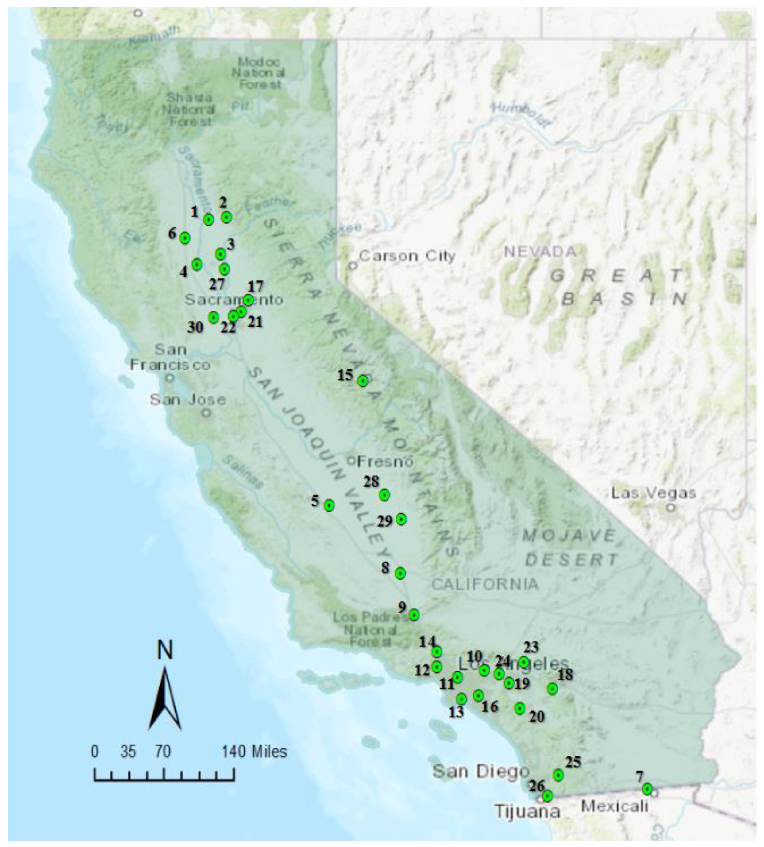
To validate the effectiveness of the proposed methodology, a case study was conducted in this paper. California, US was selected as the study area due to data availability. Hourly PM2.5 concentrations data of California from 2016 to 2017 were collected from the United States Environmental Protection Agency (EPA). Data of 30 monitoring stations were covered. A brief summary of the data is shown in

Table 1. A brief summary of the collected PM2.5 data.

Attribute	Value
Data content	PM2.5 concentrations
Temporal resolution	1 h
Location	California State, the U.S.
Duration	2016/01-2017/07
Number of stations	30
Average 1st quantile	5.3933
Average Mean	11.3668
Average Median	9.3133
Average 3rd quantile	14.7833
Average Standard Deviation	10.0275
Unit	Micrograms/Cubic Meter

. The distribution of these 30 stations is presented in Figure 2. It can be seen that the distribution is imbalanced. It is dense in the northern and southeastern areas of California but sparse in the middle areas. As mentioned in Section 0, spatial and temporal correlation of the air pollutant concentrations between two neighboring stations could be different due to the spatial distribution of stations. Take station 11 as an example. It may have higher correlation with station 12 but lower correlation with station 5 since station 5 is geospatially farther. The data from station 5 may have smaller impact on predicting the air quality in station 11 but increase the risk of noisy data contamination and lower computation speed. Therefore, it is important to consider the spatial-temporal correlation among stations when building the forecasting model. Regarding this, this paper developed a correlation filtered spatial-temporal LSTM (CFST-LSTM) model, which can automatically determine the highly correlated data segments and simultaneously optimize the model from both temporal and spatial aspects. Detailed modeling process of CFST-LSTM will be introduced later.

3.2. Data Preprocessing

After the raw data were collected, data preprocessing needed to be performed. The collected datasets unavoidably involve some missing values due to machine failure, routine maintenance, human error, insufficient sampling, and other factors. The missing values normally are required to be removed or filled to ensure the performance of modeling [35].The missing rate in this experiment was relatively small, at 2.65%. We implemented the linear interpolation methods following [36] to fill the empty values. After this procedure, each station resulted in 17,544 records of PM2.5 concentrations.

Furthermore, to mitigate the impact of dimension and speed up the model training, min-max normalization was adopted to normalize the data. Calculation of the normalization can be formulated as Equation (1)

$${\mathrm{x}}^{\ast }=\frac{\mathrm{x}-{\mathrm{x}}_{\min }}{{\mathrm{x}}_{\max }-{\mathrm{x}}_{\min }}$$

(1)

where ${\mathrm{x}}_{\max }$ represents the maximum value in the dataset and ${\mathrm{x}}_{\min }$ represents the minimum value.

3.3. Methods

3.3.1. Long Short-Term Memory (LSTM)

After the data collection and preprocessing, the modeling algorithm could be applied to model the data and predict PM2.5 concentrations. In this paper, a correlation filtered spatial-temporal long short-term memory (CFST-LSTM) model was proposed to accomplish the task. Future air quality of a target station was predicted based on the historical data of itself and surrounding stations.

The proposed CFST-LSTM network was developed based on the long short-term memory (LSTM) model. LSTM is a special architecture of recurrent neural network (RNN) proposed by Hochreiter and Schmdhuber [30]. It overcomes the vanishing and exploding gradient problem of RNN and is capable of learning from long dependencies through a gating mechanism. Due to the strong ability of LSTM in modeling temporal sequential data, it has been reported to have state-of-the-art performance in many domains, such as speech recognition, language modeling, and sequence forecasting [37,38,39,40].

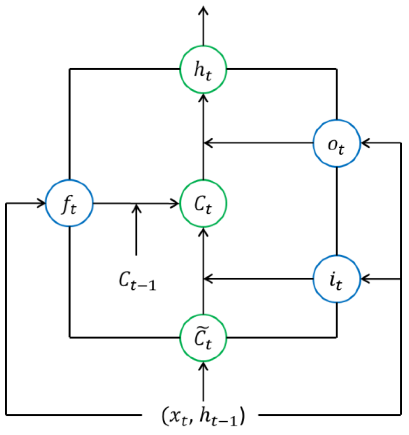
The network structure of LSTM consists of an input layer, an output layer, and a plurality of hidden layers. The specialty of LSTM lies in the compositions of its hidden layers, which are composed of one or more self-recurrent memory blocks. These blocks allow a value (forward pass) or gradient (backward pass) that flows into the block to be preserved and subsequently retrieved at the required time step [41]. The basic structure of the memory block is shown in Figure 3. It consists of three gates, including the forget gate ${\mathrm{f}}_{\mathrm{t}}$, the input gate ${\mathrm{i}}_{\mathrm{t}}$, the output gate ${\mathrm{o}}_{\mathrm{t}}$, and a recurrent connection cell ${\mathrm{C}}_{\mathrm{t}}$. ${\mathrm{x}}_{\mathrm{t}}$ is the input to the current block, ${\mathrm{h}}_{\mathrm{t}-1}$ is the hidden state of the last block, and ${\mathrm{h}}_{\mathrm{t}}$ is the state of the current block. At time step t, the LSTM memory block can be defined with the following set of equations:

$${\mathrm{f}}_{\mathrm{t}}= \mathsf{\sigma }\left({\mathrm{W}}_{\mathrm{f}}·\left[{\mathrm{h}}_{\mathrm{t}-1},{\mathrm{x}}_{\mathrm{t}}\right]+{ \mathrm{b}}_{\mathrm{f}}\right),$$

(2)

$${\mathrm{i}}_{\mathrm{t}} = \mathsf{\sigma }\left({\mathrm{W}}_{\mathrm{i}}·\left[{\mathrm{h}}_{\mathrm{t}-1},{\mathrm{x}}_{\mathrm{t}}\right]+{ \mathrm{b}}_{\mathrm{i}}\right),$$

(3)

$${\tilde{\mathrm{C}}}_{\mathrm{t}} = \tan \mathrm{h}\left({\mathrm{W}}_{\mathrm{c}}·\left[{\mathrm{h}}_{\mathrm{t}-1},{\mathrm{x}}_{\mathrm{t}}\right]+{ \mathrm{b}}_{\mathrm{c}}\right),$$

(4)

$${\mathrm{C}}_{\mathrm{t}}={\mathrm{f}}_{\mathrm{t}} ·{ \mathrm{C}}_{\mathrm{t}-1}+{\mathrm{i}}_{\mathrm{t}}·{\tilde{\mathrm{C}}}_{\mathrm{t}},$$

(5)

$${\mathrm{o}}_{\mathrm{t}}= \mathsf{\sigma }\left({\mathrm{W}}_{\mathrm{o}}·\left[{\mathrm{h}}_{\mathrm{t}-1},{\mathrm{x}}_{\mathrm{t}}\right]+{ \mathrm{b}}_{\mathrm{o}}\right),$$

(6)

$${\mathrm{h}}_{\mathrm{t}}={ \mathrm{o}}_{\mathrm{t}}·\tan \mathrm{h}\left({\mathrm{C}}_{\mathrm{t}}\right),$$

(7)

where W represents the connection weights between neurons, b represents deflection, and $\mathsf{\sigma }$ denotes the sigmoid activation the gates used.

3.3.2. CFST-LSTM

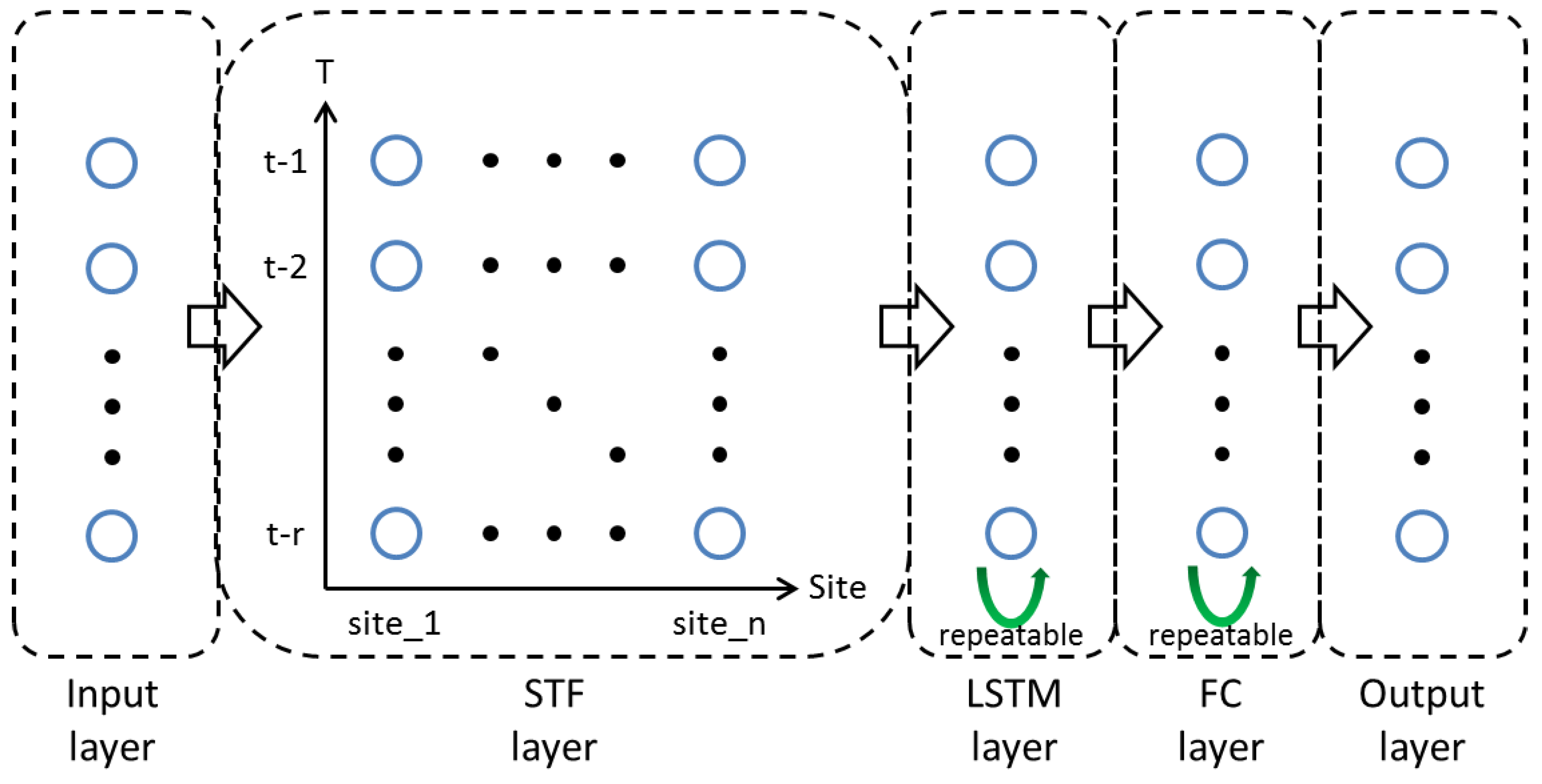
However, when predicting air pollutant concentrations, the ordinary LSTM model neither takes into account the spatial correlation among the monitoring stations nor considers the strength of the spatial-temporal correlations. Consequently, its performance is limited when the air pollution in one area is largely influenced by other areas. To overcome the problem, this study proposed a correlation filtered spatial-temporal long short-term memory (CFST-LSTM) model, which can analyze the lagged spatial-temporal correlation of the input data and select the time series data that meet the pre-set threshold. The architecture of the CFST-LSTM model is presented in Figure 4. It consists of five layers, including input layer, STF layer, LSTM layer, fully connected (FC) layer, and output layer. Working process of the CFST-LSTM model is shown as follows.

Firstly, given a dataset X, STF layer calculates the correlation coefficient matrix R for the time series of the target stations and the lagged time series of all the other stations (including the target station itself). The formulation of R is shown in Equation (8).

$$\mathrm{R}=\mathrm{Corr}\left({\mathrm{S}}_{\mathrm{target}\_\mathrm{site}},{\mathrm{S}}_{\mathrm{other}\_\mathrm{sites}}\right)$$

(8)

where $\mathrm{Corr}(·)$ denotes the function for calculating the correlation coefficient matrix, ${\mathrm{S}}_{\mathrm{target}\_\mathrm{site}}$ represents the time series of the target station, ${\mathrm{S}}_{\mathrm{other}\_\mathrm{sites}}$ represents the lagged time series matrix of other sites, which can be formulated as Equation (9).

$${\mathrm{S}}_{\mathrm{other}\_\mathrm{sites}}=\left[\begin{array}{ccc}{\mathrm{S}}_{\mathrm{site}\_1}^{\mathrm{t}-1}& \dots & {\mathrm{S}}_{\mathrm{site}\_1}^{\mathrm{t}-\mathrm{r}}\\ \dots & \dots & \dots \\ {\mathrm{S}}_{\mathrm{site}\_\mathrm{n}}^{\mathrm{t}-1}& \dots & {\mathrm{S}}_{\mathrm{site}\_\mathrm{n}}^{\mathrm{t}-\mathrm{r}}\end{array}\right]$$

(9)

where n represents the number of sites, r represents the largest time lag, t represents the length of time series, each ${\mathrm{S}}_{\mathrm{site}\_\mathrm{i}}^{\mathrm{t}-\mathrm{j}}$ represents the lagged j-moment time series of the number ith station for the target station, $1\le \mathrm{i}\le \mathrm{n}, 1\le \mathrm{j}\le \mathrm{r}$. For $\mathrm{Corr}(·)$, each ${\mathrm{R}}_{\left(\mathrm{i},\mathrm{j}\right)}=\mathsf{\rho }\left({\mathrm{S}}_{{\mathrm{target}}_{\mathrm{site}}},{\mathrm{S}}_{\mathrm{site}\_\mathrm{i}}^{\mathrm{t}-\mathrm{j}}\right)$. $\mathsf{\rho }(·)$ is the Pearson correlation function. Its calculation is shown in Equation (10).

$$\mathsf{\rho }\left(\mathrm{X},\mathrm{Y}\right)=\frac{\mathrm{Cov}\left(\mathrm{X},\mathrm{Y}\right)}{{\mathsf{\sigma }}_{\mathrm{X}}{\mathsf{\sigma }}_{\mathrm{Y}}}$$

(10)

where X represents the original input of the model, Y represents the output, $\mathrm{Cov}\left(\mathrm{X},\mathrm{Y}\right)$ represents the covariance of X and Y, ${\mathsf{\sigma }}_{\mathrm{X}}$ and ${\mathsf{\sigma }}_{\mathrm{Y}}$ represent the standard deviation of X and Y, respectively, $\mathsf{\rho }\in \left(-1,1\right)$. The formulation of X can be expressed as Equation (11).

$$\mathrm{X}=\left[\begin{array}{ccc}\mathrm{site}\_1^{\mathrm{t}-1}& \dots & \mathrm{site}\_1^{\mathrm{t}-\mathrm{r}}\\ \dots & \dots & \dots \\ \mathrm{site}\_{\mathrm{n}}^{\mathrm{t}-1}& \dots & \mathrm{site}\_{\mathrm{n}}^{\mathrm{t}-\mathrm{r}}\end{array}\right]$$

(11)

where $\mathrm{site}\_{\mathrm{i}}^{\mathrm{t}-\mathrm{j}}$ represents the recorded value of the ith station at time t-j.

Secondly, transform the R based on the correlation threshold ${\mathsf{\rho }}_{\mathrm{th}}$, as shown in Equation (12).

$${\mathrm{R}}^{\mathrm{I}}=\mathrm{I}\left(\mathrm{R},{\mathsf{\rho }}_{\mathrm{th}}\right)$$

(12)

where $\mathrm{I}(·)$ represents the indicator function. When ${\mathrm{R}}_{\left(\mathrm{i},\mathrm{j}\right)}\ge {\mathsf{\rho }}_{\mathrm{th}}$, ${\mathrm{R}}_{\left(\mathrm{i},\mathrm{j}\right)}^{\mathrm{I}}=1$. When ${\mathrm{R}}_{\left(\mathrm{i},\mathrm{j}\right)}<{\mathsf{\rho }}_{\mathrm{th}}$, ${\mathrm{R}}_{\left(\mathrm{i},\mathrm{j}\right)}^{\mathrm{I}}=0$.

Thirdly, apply the element-wise product to X and ${\mathrm{R}}^{\mathrm{I}}$. Then, the final output ${\mathrm{X}}^{\prime }$ of STF layer is given, as presented in Equation (13).

$${\mathrm{X}}^{\prime }={\left({\mathrm{X}\ast \mathrm{R}}^{\mathrm{I}}\right)}^{\mathrm{T}}$$

(13)

where $\ast$ represents the element-wise product and ${(·)}^{\mathrm{T}}$ represents the matrix transpose.

After the ${\mathrm{X}}^{\prime }$ is given, it is input into the LSTM layer. The following steps are the same as the ordinary LSTM model.

4. Results and Discussions

4.1. LSTM Structure Optimization

To validate the effectiveness of the proposed model, hourly PM2.5 data of 30 stations in California were collected. After the data were preprocessed, they were input into the model. However, before that, parameters of the model need to be optimized at first. For illustration purpose, monitoring station 11 is used as an example. It contains 17,544 records of PM2.5 concentrations; 70% of its data are used as training samples while the remained 30% are used as testing samples. The number of samples relies on the largest time lag value. If time lag is 12, then there will have 12,272 training samples, and 5260 testing samples. Note that the calculated optimization results in the following paper are all based on the performance from the testing set.

Before applying the proposed model on further experiments, its parameters need to be identified and optimized for a better result. Although this study designed an STF layer into the LSTM network, some parameters of the deep neural network setting can be re-used. Following the study of V et al., [42], this paper sets the epoch and batch size as 1000 and 48, respectively. MSE is selected as the loss function, and RMSprop is adopted as the optimizer. The learning rate of the model is set as 0.001. The number of fully connected layer is set as 1. The number of neurons of fully connected layer is set as 64. The linear active function is used. The number of neurons of output layer is set as 1. The discussion on the largest time lag of STF layer and ${\mathsf{\rho }}_{\mathrm{threshold}}$ will be introduced in later sections, and we pre-set them as 12 and 0.4 first.

The most important parameters that need to be tuned before model implementation is the structure of the stacked LSTM layer. The optimization performance is evaluated using root mean square error (RMSE), mean absolute error (MAE), and ${\mathrm{R}}^2$. Calculations of the three metrics are presented in Equations (14), (15) and (16), respectively.

$$\mathrm{RMSE}=\sqrt{\frac{1}{\mathrm{N}}{\displaystyle \sum }_{\mathrm{i}=1}^{\mathrm{N}}{\left({\mathrm{y}}_{\mathrm{true}}^{\mathrm{i}}-{\mathrm{y}}_{\mathrm{pred}}^{\mathrm{i}}\right)}^2}$$

(14)

$$\mathrm{MAE}=\frac{1}{\mathrm{N}}{\displaystyle \sum }_{\mathrm{i}=1}^{\mathrm{N}}|{\mathrm{y}}_{\mathrm{true}}^{\mathrm{i}}-{\mathrm{y}}_{\mathrm{pred}}^{\mathrm{i}}|$$

(15)

$${\mathrm{R}}^2=1-\frac{{{\displaystyle \sum }}_{\mathrm{i}=1}^{\mathrm{N}}{\left({\mathrm{y}}_{\mathrm{true}}^{\mathrm{i}}-{\mathrm{y}}_{\mathrm{pred}}^{\mathrm{i}}\right)}^2}{{{\displaystyle \sum }}_{\mathrm{i}=1}^{\mathrm{N}}{\left({\mathrm{y}}_{\mathrm{true}}^{\mathrm{i}}-{\mathrm{y}}_{\mathrm{mean}}^{\mathrm{true}}\right)}^2}$$

(16)

where N represents the number of samples, ${\mathrm{y}}_{\mathrm{true}}^{\mathrm{i}}$ represents the true value of the ith sample, ${\mathrm{y}}_{\mathrm{pred}}^{\mathrm{i}}$ represents the predicted value of the ith sample, and ${\mathrm{y}}_{\mathrm{mean}}^{\mathrm{true}}$ represents the mean value of true values.

The number of neurons in each LSTM layer is set as the same. Candidates of the number of LSTM layers narrowed down to {2–4} after a trial and error process, and the number of neurons at each layer was set as {32, 64, 128}. Optimization results are shown in

Table 2. Optimization of the structure of the LSTM layer.

Layers	Nodes	RMSE $(\mathsf{\mu }\mathbf{g}/{\mathit{m}}^3)$	MAE $(\mathsf{\mu }\mathbf{g}/{\mathit{m}}^3)$	${\mathbf{R}}^2$
2	32	2.0122	1.5385	0.9534
	64	1.9926	1.5161	0.9583
	128	2.1270	1.5687	0.9477
3	32	2.1156	1.6306	0.9483
	64	2.0934	1.5553	0.9494
	128	2.1378	1.6026	0.9471
4	32	2.1632	1.6269	0.9458
	64	2.1998	1.6904	0.9439
	128	2.1744	1.7027	0.9453

. It can be observed that when the number of LSTM layers is 2 and the number of neurons of each layer is 64, the model has the lowest scores of RMSE and MAE and the highest score of ${\mathrm{R}}^2$. Therefore, this paper sets the number of LSTM layers as 2 and the number of neurons as 64.

4.2. Comparison of Different Correlation Threshold

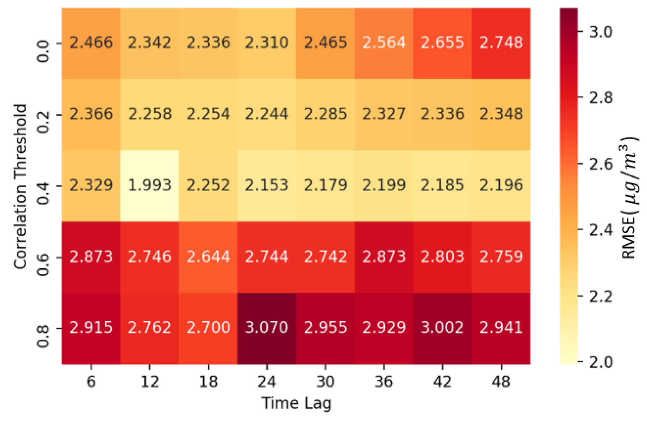
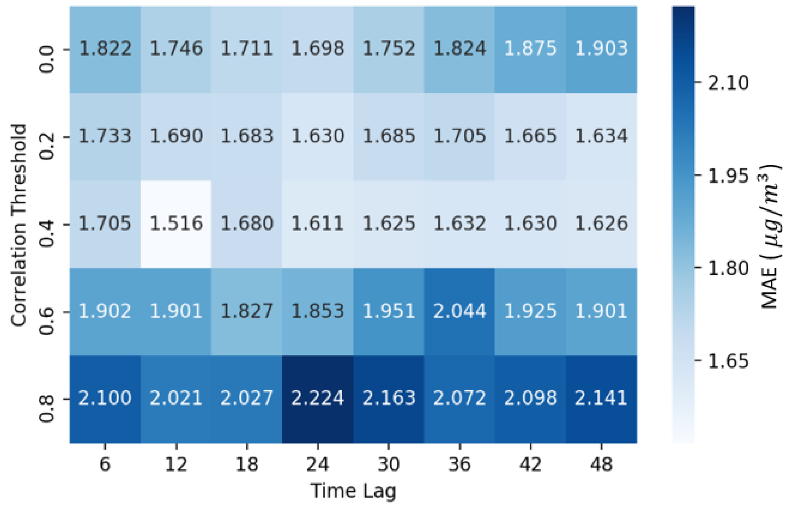
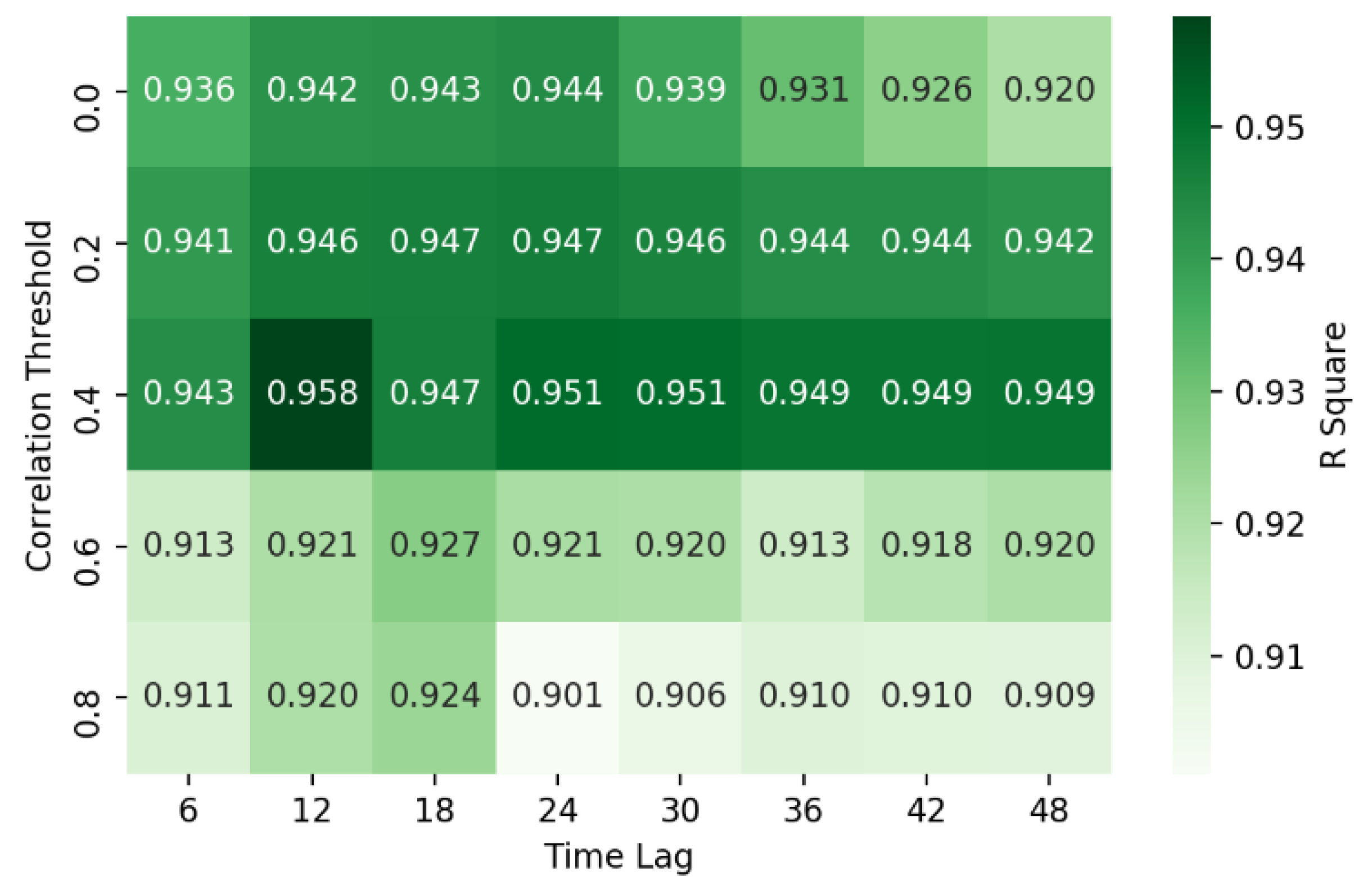
Besides the structure of the stacked LSTM layer, it is also important to optimize the largest time lag r and correlation threshold ${\mathsf{\rho }}_{\mathrm{th}}$. These two parameters are the key parameters in the newly designed STF layer. Time lag r decided the feature pool of the model. Correlation threshold ${\mathsf{\rho }}_{\mathrm{th}}$ decided the quality of the feature pool. Since the air quality time series pattern in one place usually follows a daily period, and one day may not enough to extract the useful pattern, we therefore set the test range of r as 48 h, and calculated the model performance using different pairs of r and ${\mathsf{\rho }}_{\mathrm{th}}$. The results are shown in Figure 5, Figure 6 and Figure 7.

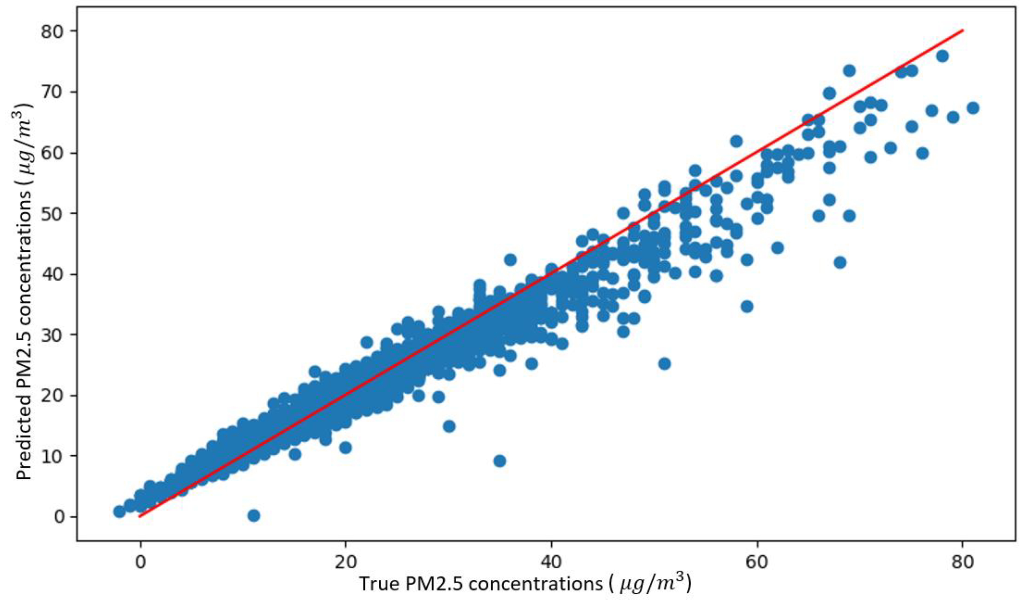
It can be seen from Figure 5, Figure 6 and Figure 7 that both two parameters can affect the model performance a lot. For example, the ${\mathrm{R}}^2$ value can change from the lowest 0.909 to 0.958. It is almost 5% performance. The setting of ${\mathsf{\rho }}_{\mathrm{th}}$ shows a clear separation for model performance. When ${\mathsf{\rho }}_{\mathrm{th}}$ ≤ 0.4, the ${\mathrm{R}}^2$ value never gets lower than 0.920, and when ${\mathsf{\rho }}_{\mathrm{th}}>0.4$, most of the ${\mathrm{R}}^2$ values are lower than 0.920. This is because when ${\mathsf{\rho }}_{\mathrm{th}}$ is too large, many useful inputs will be filtered out, and result in limited knowledge to learn. But when ${\mathsf{\rho }}_{\mathrm{th}}$ goes too low, the inputs will keep much noise, and therefore the model performance drops. Overall, it can be seen from Figure 5, Figure 6 and Figure 7 that when r = 12, and ${\mathsf{\rho }}_{\mathrm{th}}$ = 0.4, the model has the lowest RMSE, MAE and highest ${\mathrm{R}}^2$ value. This pair is then the optimal pair for these two parameters. The goodness of fit plot is shown in Figure 8.

4.3. Model Comparison

To prove the effectiveness of the CFST-LSTM model, its prediction performance is compared with other traditional machine learning models and commonly seen neural networks. These contain three traditional machine learning models, including LASSO regression, Ridge regression, and support vector regression (SVR), and two commonly seen neural networks, including artificial neural network (ANN) and recurrent neural network (RNN) [43,44,45,46,47]. The parameters of these algorithms were all tuned using the same grid search process.

Table 3. Model comparison.

Model	RMSE $(\mathsf{\mu }\mathbf{g}/{\mathit{m}}^3)$	MAE $(\mathsf{\mu }\mathbf{g}/{\mathit{m}}^3)$	${\mathbf{R}}^2$
LASSO	2.93213	1.951243	0.915126
Ridge	2.89453	1.932423	0.918705
SVR	2.79312	1.892831	0.925028
ANN	2.78484	1.882643	0.925734
RNN	2.70294	1.853425	0.929810
CFST-LSTM	1.99257	1.516072	0.958348
CFST-ANN	2.62591	1.79819	0.930665
CFST-RNN	2.53594	1.70958	0.939712

presents the results of the model comparison. (1) It can be seen from the first six rows that compared with other models, the two deep learning neural networks, RNN and CFST-LSTM, have lower RMSE/MAE and higher ${\mathrm{R}}^2$. This is because compared with Lasso and Ridge, neural network-based learning algorithms are better at modeling non-linear real-world relationships. Therefore, ANN, RNN, and CFST-LSTM have better performance. (2) Also, compared with traditional machine learning methods SVR and ANN, the other two deep learning based models (RNN and CFST-LSTM) have lower error and higher ${\mathrm{R}}^2$. This is because they are specifically designed for time series problems. It is easier for them to learn the impact from historical data. (3) Lastly, CFST-LSTM outperforms RNN, and exhibits the lowest RMSE and the highest ${\mathrm{R}}^2$. It can be seen that the difference is quite significant. The main reason is that except CFST-LSTM, other models did not consider the influence from nearby stations.

Since the newly designed STF layer in CFST-LSTM is one kind of neural network layer, it can also be added into ANN and RNN. To test how much it can help increase the performance of neural network models, this study also calculated the ${\mathrm{R}}^2$ value of CFST-ANN and CFST-RNN. The results are shown in the last two columns in Table 3. It can be seen that the ${\mathrm{R}}^2$ values of these two neural networks have improved. This, on another angle, proved the effectiveness of the proposed STF layer. However, the overall performance of CFST-ANN and CFST-RNN are still behind CFST-LSTM. This is because the LSTM layer in CFST-LSTM is better at learning long-term dependency from time series data.

4.4. Comparison of Ordinary LSTM and CFST-LSTM

Besides the comparison between CFST-LSTM and other commonly seen machine learning/deep learning algorithms, this study also compared the performance of CFST-LSTM and the ordinary LSTM network. To better illustrate the comparison and the advantages of the proposed CFST-LSTM model, this experiment expands the test site form site 11 to all the sites within California State. For each site, we will separate the data into 70% training set and 30% testing set, and then train the models using ordinary LSTM (O-LSTM), full site inputs LSTM (F-LSTM), and CFST-LSTM. The differences between these three models are shown in Equations (17) to (19).

$$Input{s}_{Site i}\stackrel{O-LSTM}{\to }Prediction{s}_{Site i}$$

(17)

$$Input{s}_{All Sites}\stackrel{F-LSTM}{\to }Prediction{s}_{Site i}$$

(18)

$$Input{s}_{All Sites}\stackrel{CFST-LSTM}{\to }Prediction{s}_{Site i}$$

(19)

The results are all calculated based on the testing sets of different sites, and they are shown in Figure 9. Figure 9 (left) is the ${\mathrm{R}}^2$ values on different sites. $R_O^2$ means the ${\mathrm{R}}^2$ value calculated using O-LSTM, and is marked using a blue line. $R_F^2$ means F-LSTM, and is marked using a green line. $R_C^2$ means CFST-LSTM, and is presented using an orange line. It can be seen that overall, CFST-LSTM performs the best, O-LSTM the second, and F-LSTM the third. To show the difference between these three models more clear, we calculated the values of $R_O^2-R_F^2$ and $R_O^2-R_C^2$, and also plotted them on Figure 9 (right). In this way, it can be seen that O-LSTM performs better than F-LSTM in most sites, while it also seldom surpasses CFST-LSTM.

The average values of these three indicators on all sites are shown in

Table 4. Average R Square value of different LSTM models on all sites.

Models	CFST-LSTM	O-LSTM	F-LSTM
Average R Square	0.9155	0.8899	0.8613

. It can be seen that CFST-LSTM has the highest average ${\mathrm{R}}^2$ with a value of 0.9155, and it is 2.88% better than O-LSTM and 6.29% better than F-LSTM. This is reasonable since CFST-LSTM not only considered the influence from nearby stations, but also filtered out less related time series inputs. F-LSTM performs the worst with a value of 0.8613, which is 3.32% lower than O-LSTM. This is also understandable since it contains too much noise when modeling the PM2.5 concentrations.

Overall, the comparison between these three models helps prove the effectiveness of the proposed CFST-LSTM. This reflects that retaining the stations with higher correlation and dropping those with lower correlation can effectively improve the prediction accuracy of PM2.5 concentrations.

4.5. Improvements Interpolation

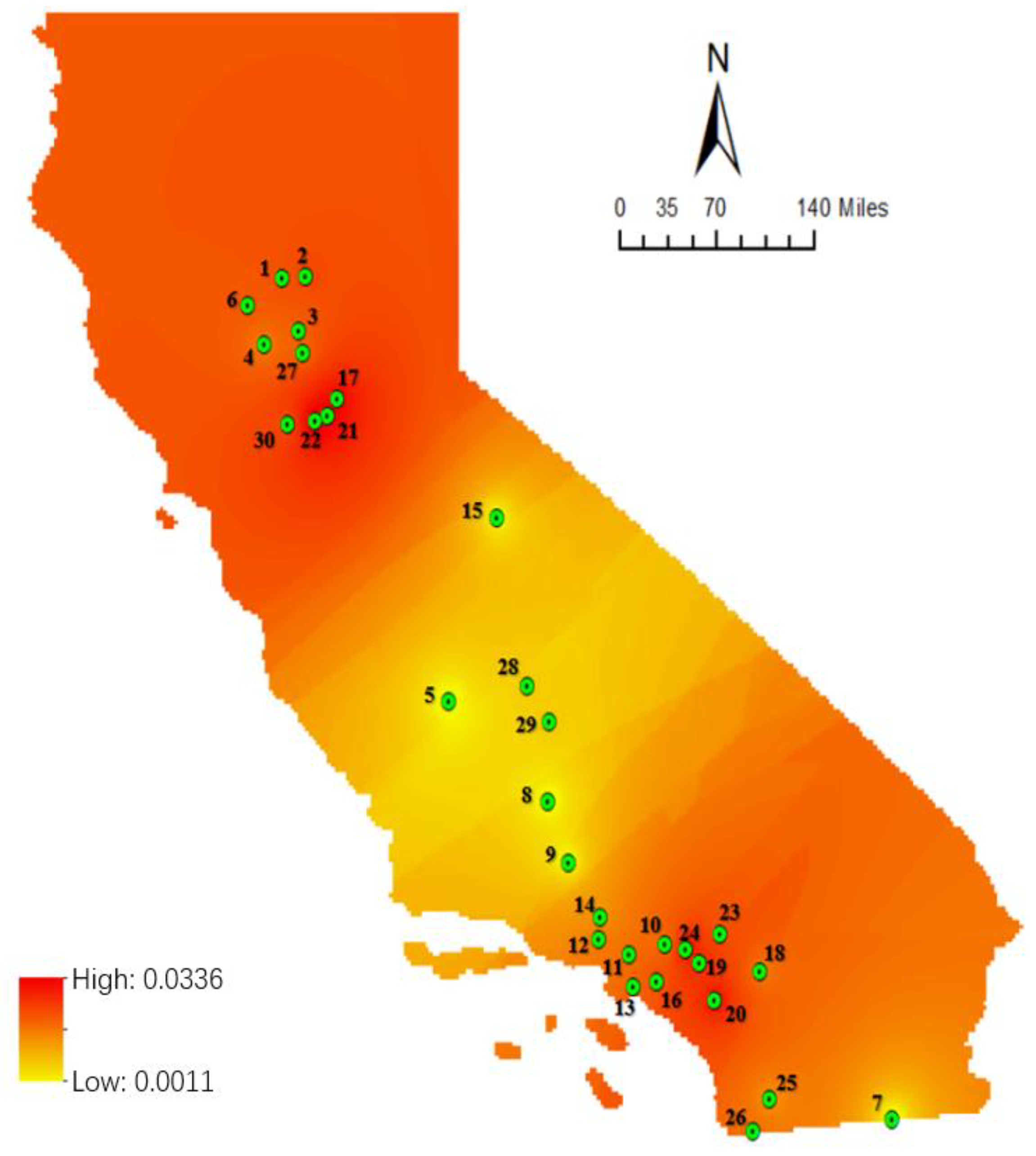
To further explore the features of CFST-LSTM, this study interpolates the ${\mathrm{R}}^2$ improvements geospatially. The inverse distance weighted (IDW) technique of GIS [48] is used to visualize and interpolate the value of $R_{\Delta }^2=R_C^2-R_O^2$ in the map of California. The spatial change of $R_{\Delta }^2$ is presented in Figure 10. Red means the value of $R_{\Delta }^2$ is high while yellow means the value of $R_{\Delta }^2$ is low. It can be seen that for areas with denser stations, the improvement is higher than those with sparser stations. This is because in areas with higher density of stations, more stations remained during the modeling process of CFST-LSTM, and therefore more related information are utilized to learn the temporal patterns. However, in areas with lower density of stations, only one or two stations might be retained by CFST-LSTM as the inputs. The prediction result, therefore, could be similar to the ordinary model, which uses the historical data of the target station only.

5. Conclusions

This paper proposed a correlation filtered spatial-temporal long short-term memory (CFST-LSTM) model for PM2.5 concentrations prediction. For a target station, not only the historical data of itself, but also the data of its surrounding stations are used. A spatial-temporal filter (STF) layer was designed to automatically remove the station data with low correlation with the target station. Hourly PM2.5 concentrations data of 30 stations in California were collected to validate the model effectiveness. Prediction performance of the CFST-LSTM model was compared with other traditional machine learning models and commonly seen neural networks. Results show that:

• The proposed CFST-LSTM model outperforms other commonly seen machine learning/deep learning models with a better fitting degree and higher prediction accuracy. Its ${\mathrm{R}}^2$ can reach 0.9583.
• Compared with ordinary LSTM, our method not only considers the influence from nearby stations but also filters out less related time series inputs, and this helps increase 2.88% ${\mathrm{R}}^2$ performance in our tests on 30 sites. On the other hand, if only simply adding the time series inputs from other stations, the model performance will drop 3.32% due to a higher level of noise.
• According to the experiment on the ${\mathrm{R}}^2$ improvements over the sites in California, the proposed method exhibited a higher improvement over ordinary LSTM in areas with denser sites, but lower improvement in sparser districts. This reflects that our method performs better at places with denser spatial inputs.
• Parameter optimization of the newly designed STF layer is quite important to the proposed method. The experiment showed that the difference in ${\mathrm{R}}^2$ between proper and improper parameters can reach around 5.39% of the overall performance.

The main contribution of this study is that we proposed an improved neural network model for spatial-temporal time series predictions. The model is modified based on deep learning techniques. Besides the prediction of PM2.5 concentrations, the model is expected to be applicable to other types of spatial-temporal time series problems, such as the prediction of weather, wind power, and other types of air pollutants. Of course, further studies need to be conducted for verifications.

Due to the data availability, only the historical PM2.5 concentration data are collected and tested in this paper. Other possible influential factors of PM2.5, such as meteorological characteristics and traffic emissions, are not considered. Further studies could be conducted to explore the feasibility of implementing the proposed method on multivariate inputs.

References

1. Cakmak, S.; Dales, R.E.; Rubio, M.A.; Vidal, C.B. The risk of dying on days of higher air pollution among the socially disadvantaged elderly. Environ. Res. 2011, 111, 388–393. [Google Scholar] [CrossRef]
2. Bai, L.; He, Z.; Li, C.; Chen, Z. Investigation of yearly indoor/outdoor PM2.5 levels in the perspectives of health impacts and air pollution control: Case study in Changchun, in the northeast of China. Sustain. Cities Soc. 2019, 101871. [Google Scholar] [CrossRef]
3. Xia, Y.; Guan, D.; Jiang, X.; Peng, L.; Schroeder, H.; Zhang, Q. Assessment of socioeconomic costs to China’s air pollution. Atmos. Environ. 2016, 139, 147–156. [Google Scholar] [CrossRef]
4. Lin, C.; Lau, A.K.H.; Fung, J.C.H.; He, Q.; Ma, J.; Lu, X.; Li, Z.; Li, C.; Zuo, R.; Wong, A.H.S. Decomposing the Long-term Variation in Population Exposure to Outdoor PM2.5 in the Greater Bay Area of China Using Satellite Observations. Remote Sens. 2019, 11, 2646. [Google Scholar] [CrossRef] [Green Version]
5. Tiwari, A.; Kumar, P.; Baldauf, R.; Zhang, K.M.; Pilla, F.; Di Sabatino, S.; Brattich, E.; Pulvirenti, B. Considerations for evaluating green infrastructure impacts in microscale and macroscale air pollution dispersion models. Sci. Total. Environ. 2019, 672, 410–426. [Google Scholar] [CrossRef] [PubMed] [Green Version]
6. Ma, J.; Ding, Y.; Cheng, J.C.P.; Jiang, F.; Tan, Y.; Gan, V.J.L.; Wan, Z. Identification of high impact factors of air quality on a national scale using big data and machine learning techniques. J. Clean. Prod. 2019, 118955. [Google Scholar] [CrossRef]
7. Zhao, D.; Chen, H.; Li, X.; Ma, X. Air pollution and its influential factors in China’s hot spots. J. Clean. Prod. 2018, 185, 619–627. [Google Scholar] [CrossRef]
8. Ma, J.; Cheng, J.C.P.; Lin, C.; Tan, Y.; Zhang, J. Improving air quality prediction accuracy at larger temporal resolutions using deep learning and transfer learning techniques. Atmos. Environ. 2019, 214, 116885. [Google Scholar] [CrossRef]
9. Ma, J.; Ding, Y.; Gan, V.J.L.; Lin, C.; Wan, Z. Spatiotemporal Prediction of PM2.5 Concentrations at Different Time Granularities Using IDW-BLSTM. IEEE Access 2019, 7, 107897–107907. [Google Scholar] [CrossRef]
10. Davis, J.M.; Speckman, P. A model for predicting maximum and 8h average ozone in Houston. Atmos. Environ. 1999, 33, 2487–2500. [Google Scholar] [CrossRef]
11. Liu, T.; Lau, A.K.H.; Sandbrink, K.; Fung, J.C.H. Time Series Forecasting of Air Quality Based On Regional Numerical Modeling in Hong Kong. J. Geophys. Res. Atmos. 2018, 123, 4175–4196. [Google Scholar] [CrossRef] [Green Version]
12. Kulkarni, G.E.; Muley, A.A.; Deshmukh, N.K.; Bhalchandra, P.U. Autoregressive integrated moving average time series model for forecasting air pollution in Nanded city, Maharashtra, India. Model. Earth Syst. Environ. 2018, 4, 1435–1444. [Google Scholar] [CrossRef]
13. Osowski, S.; Garanty, K. Forecasting of the daily meteorological pollution using wavelets and support vector machine. Eng. Appl. Artif. Intell. 2007, 20, 745–755. [Google Scholar] [CrossRef]
14. Gardner, M.W.; Dorling, S.R. Neural network modelling and prediction of hourly NOx and NO2 concentrations in urban air in London. Atmos. Environ. 1999, 33, 709–719. [Google Scholar] [CrossRef]
15. Jusoh, N.; Ibrahim, W.J.W. Evaluating Fuzzy Time Series and Artificial Neural Network for Air Pollution Index Forecasting. In Proceedings of the Second International Conference on the Future of ASEAN (ICoFA) 2017—Volume 2; Saian, R., Abbas, M.A., Eds.; Springer: Singapore, 2018; pp. 113–121. [Google Scholar]
16. Prakash, A.; Kumar, U.; Kumar, K.; Jain, V.K. A Wavelet-based Neural Network Model to Predict Ambient Air Pollutants’ Concentration. Environ. Model. Assess 2011, 16, 503–517. [Google Scholar] [CrossRef]
17. Li, X.; Peng, L.; Yao, X.; Cui, S.; Hu, Y.; You, C.; Chi, T. Long short-term memory neural network for air pollutant concentration predictions: Method development and evaluation. Environ. Pollut. 2017, 231, 997–1004. [Google Scholar] [CrossRef]
18. Yang, W.; Deng, M.; Xu, F.; Wang, H. Prediction of hourly PM2.5 using a space-time support vector regression model. Atmos. Environ. 2018, 181, 12–19. [Google Scholar] [CrossRef]
19. Szpiro, A.A.; Sampson, P.D.; Sheppard, L.; Lumley, T.; Adar, S.D.; Kaufman, J.D. Predicting intra-urban variation in air pollution concentrations with complex spatio-temporal dependencies. Environ. 2010, 21, 606–631. [Google Scholar] [CrossRef] [Green Version]
20. Deep Learning. Wikipedia. 2019. Available online: https://en.wikipedia.org/w/index.php?title=Deep_learning&oldid=887765315 (accessed on 18 March 2019).
21. Ma, J.; Ding, Y.; Cheng, J.C.P.; Tan, Y.; Gan, V.J.L.; Zhang, J. Analyzing the Leading Causes of Traffic Fatalities Using XGBoost and Grid-Based Analysis: A City Management Perspective. IEEE Access 2019, 7, 148059–148072. [Google Scholar] [CrossRef]
22. Ma, J.; Cheng, J.C.P. Identification of the numerical patterns behind the leading counties in the U.S. local green building markets using data mining. J. Clean. Prod. 2017, 151, 406–418. [Google Scholar] [CrossRef]
23. Schmidhuber, J. Deep learning in neural networks: An overview. Neural Netw. 2015, 61, 85–117. [Google Scholar] [CrossRef] [PubMed] [Green Version]
24. Singh, K.P.; Gupta, S.; Rai, P. Identifying pollution sources and predicting urban air quality using ensemble learning methods. Atmos. Environ. 2013, 80, 426–437. [Google Scholar] [CrossRef]
25. Wang, W.; Men, C.; Lu, W. Online prediction model based on support vector machine. Neurocomputing 2008, 71, 550–558. [Google Scholar] [CrossRef]
26. Russo, A.; Raischel, F.; Lind, P.G. Air quality prediction using optimal neural networks with stochastic variables. Atmos. Environ. 2013, 79, 822–830. [Google Scholar] [CrossRef] [Green Version]
27. Kumar, R.; Aggarwal, R.K.; Sharma, J.D. Energy analysis of a building using artificial neural network: A review. Energy Build. 2013, 65, 352–358. [Google Scholar] [CrossRef]
28. Tealab, A. Time series forecasting using artificial neural networks methodologies: A systematic review. Future Comput. Inform. J. 2018, 3, 334–340. [Google Scholar] [CrossRef]
29. Ma, J.; Ding, Y.; Cheng, J.C.P.; Jiang, F.; Wan, Z. A temporal-spatial interpolation and extrapolation method based on geographic Long Short-Term Memory neural network for PM2.5. J. Clean. Prod. 2019, 237, 117729. [Google Scholar] [CrossRef]
30. Hochreiter, S.; Schmidhuber, J. Long Short-Term Memory. Neural Comput. 1997, 9, 1735–1780. [Google Scholar] [CrossRef]
31. Azzouni, A.; Pujolle, G. A Long Short-Term Memory Recurrent Neural Network Framework for Network Traffic Matrix Prediction. arXiv 2017, arXiv:170505690. Available online: http://arxiv.org/abs/1705.05690 (accessed on 29 September 2018).
32. Ma, J.; Ding, Y.; Cheng, J.C.P.; Jiang, F.; Xu, Z. Soft detection of 5-day BOD with sparse matrix in city harbor water using deep learning techniques. Water Res. 2019, 170, 115350. [Google Scholar] [CrossRef]
33. Peng, L.; Liu, S.; Liu, R.; Wang, L. Effective long short-term memory with differential evolution algorithm for electricity price prediction. Energy 2018, 162, 1301–1314. [Google Scholar] [CrossRef]
34. Salman, A.G.; Heryadi, Y.; Abdurahman, E.; Suparta, W. Single Layer & Multi-layer Long Short-Term Memory (LSTM) Model with Intermediate Variables for Weather Forecasting. Procedia Comput. Sci. 2018, 135, 89–98. [Google Scholar] [CrossRef]
35. Ma, J.; Cheng, J.C.P. Estimation of the building energy use intensity in the urban scale by integrating GIS and big data technology. Appl. Energy 2016, 183, 182–192. [Google Scholar] [CrossRef]
36. Junninen, H.; Niska, H.; Tuppurainen, K.; Ruuskanen, J.; Kolehmainen, M. Methods for imputation of missing values in air quality data sets. Atmos. Environ. 2004, 38, 2895–2907. [Google Scholar] [CrossRef]
37. Graves, A.; Fernández, S.; Schmidhuber, J. Bidirectional LSTM Networks for Improved Phoneme Classification and Recognition. In Artificial Neural Networks: Formal Models and Their Applications—ICANN 2005, Warsaw, Poland, 11–15 September 2005; Duch, W., Kacprzyk, J., Oja, E., Zadrożny, S., Eds.; Springer: Berlin/Heidelberg, Germany, 2005; pp. 799–804. [Google Scholar]
38. Ma, J.; Li, Z.; Cheng, J.C.P.; Ding, Y.; Lin, C.; Xu, Z. Air quality prediction at new stations using spatially transferred bi-directional long short-term memory network. Sci. Total Environ. 2019, 135771. [Google Scholar] [CrossRef]
39. Graves, A.; Jaitly, N.; Mohamed, A. Hybrid speech recognition with Deep Bidirectional LSTM. In Proceedings of the 2013 IEEE Workshop Autom. Speech Recognit. Underst., Olomouc, Czech Republic, 8–12 December 2013; pp. 273–278. [Google Scholar] [CrossRef]
40. Shi, X.; Chen, Z.; Wang, H.; Yeung, D.Y.; Wong, W.; Woo, W. Convolutional LSTM Network: A Machine Learning Approach for Precipitation Nowcasting. In Advances in Neural Information Processing 28; Cortes, C., Lawrence, N.D., Lee, D.D., Sugiyama, M., Garnett, R., Eds.; The MIT Press: Cambridge, MA, USA; London, UK, 2015; pp. 802–810. Available online: http://papers.nips.cc/paper/5955-convolutional-lstm-network-a-machine-learning-approach-for-precipitation-nowcasting.pdf (accessed on 7 September 2018).
41. Bengio, Y.; Simard, P.; Frasconi, P. Learning long-term dependencies with gradient descent is difficult. IEEE Trans. Neural Netw. Learn. Syst. 1994, 5, 157–166. [Google Scholar] [CrossRef]
42. Athira, V.; Geetha, P.; Vinayakumar, R.; Soman, K.P. DeepAirNet: Applying Recurrent Networks for Air Quality Prediction. Procedia Comput. Sci. 2018, 132, 1394–1403. [Google Scholar] [CrossRef]
43. Ma, J.; Cheng, J.C.P. Identifying the influential features on the regional energy use intensity of residential buildings based on Random Forests. Appl. Energy 2016, 183, 193–201. [Google Scholar] [CrossRef]
44. Cheng, J.C.P.; Ma, L.J. A data-driven study of important climate factors on the achievement of LEED-EB credits. Build. Environ. 2015, 90, 232–244. [Google Scholar] [CrossRef]
45. Cheng, J.C.P.; Ma, L.J. A non-linear case-based reasoning approach for retrieval of similar cases and selection of target credits in LEED projects. Build. Environ. 2015, 93, 349–361. [Google Scholar] [CrossRef]
46. Ma, J.; Cheng, J.C.P. Data-driven study on the achievement of LEED credits using percentage of average score and association rule analysis. Build. Environ. 2016, 98, 121–132. [Google Scholar] [CrossRef]
47. Jun, M.A.; Cheng, J.C.P. Selection of target LEED credits based on project information and climatic factors using data mining techniques. Adv. Eng. Inform. 2017, 32, 224–236. [Google Scholar] [CrossRef]
48. Inverse Distance Weighting, Wikipedia. 2018. Available online: https://en.wikipedia.org/w/index.php?title=Inverse_distance_weighting&oldid=834154831 (accessed on 7 September 2018).
Figure 1. Research framework.
Applsci 10 00014 g001
Figure 2. The distribution and code number of the 30 stations.
Applsci 10 00014 g002
Figure 3. The basic structure of the long short-term memory (LSTM) memory block.
Applsci 10 00014 g003
Figure 4. The architecture of the correlation filtered spatial-temporal long short-term memory (CFST-LSTM) model.
Applsci 10 00014 g004
Figure 5. Root mean square error (RMSE) values of the model using different pairs of r and ρ th .
Applsci 10 00014 g005
Figure 6. Mean absolute error (MAE) values of the model using different pairs of r and ρ th .
Applsci 10 00014 g006
Figure 7. R 2 values of the model using different pairs of r and ρ th .
Applsci 10 00014 g007
Figure 8. The goodness of fit plot of the CFST-LSTM model.
Applsci 10 00014 g008
Figure 9. Comparison of different LSTM models on different sites.
Applsci 10 00014 g009
Figure 10. The spatial interpolation of R Δ 2 in California State.
Applsci 10 00014 g010