Modeling the Connection between Bank Systemic Risk and Balance-Sheet Liquidity Proxies through Random Forest Regressions

Abstract

Balance-sheet indicators may reflect, to a great extent, bank fragility. This inherent relationship is the object of theoretical models testing for balance-sheet vulnerabilities. In this sense, we aim to analyze whether systemic risk for a sample of US banks can be explained by a series of balance-sheet variables, considered as proxies for bank liquidity for the 2004:1–2019:1 period. We first compute Marginal Expected Shortfall values for the entities in our sample and then imbed them into a Random Forest regression setup. Although we discover that feature importance is rather bank-specific, we notice that cash and available-for-sale securities are the most relevant factors in explaining the dynamics of systemic risk. Our findings emphasize the need for heightened prudential regulation of bank liquidity, particularly in what concerns cash and immediate liquidity instrument weights. Moreover, systemic risk could be consistently tamed by consolidating bank emergency liquidity provision schemes.

1. Introduction

The recent global crisis that showed strong credit and liquidity issues motivated bank supervisors and regulators to reconsider the basics of banking regulations. The general approach of considering the health of individual banks was appended with previsions of macro-prudential measures in a bid to deter potential systemic risk problems. There is a consensus about the fact that systemic risk generates negative externalities in the financial system that cannot be internalized by individual institutions. Negative shocks to bank capital are usually followed by asset selling and adjustments in lending. As capital shortages are rarely specific to one bank, such situations can amplify the impact of the original shock, so that systemic risk induces an overall scarcity of capital in the financial sector. As highlighted by Buch et al. (2019) systemic risk expansion is catalyzed by the tendency of banks to be undercapitalized at moments when the entire financial system is undercapitalized, which further motivates the need for macro-prudential instruments.

The issue of systemic risk is anything but new for financial markets. However, the attention of academia and policymakers has been draught towards systemic risk only recently, when the 2008 financial crisis proved that it has been, yet again, conspicuously underestimated. The 2008 crisis actually represented a turning point for research targeting the causes, accumulation, spread, or mitigation of system-wide risks.

Expected shortfall methods gained great popularity with the onset of the crisis and kept being intensively used due to their ease and friendly data requirements. Perhaps the widest body of literature dealing with systemic risk measurement ever since has resorted to Conditional Capital Shortfall methods. The seminal work of Acharya et al. (2010) put forward the Marginal Expected Shortfall, which measures the expected loss of a firm conditional on the system being in distress, and is calculated using the lower 5% quantile of returns of the value-weighted market index. Several other works have followed their footsteps and used Marginal Expected Shortfall based methodologies to tackle systemic risk issues (Idier et al. 2014; Billio et al. 2016; Kleinow et al. 2017; Lin et al. 2018). Many of them used Marginal Expected Shortfall based methods as explicit risk measurement tools in various instances (see Engle et al. 2014; Ben Ameur et al. 2017; Battaglia and Gallo 2013), while others took on the challenge of testing their performance in measuring systemic risk: Pederzoli and Torricelli (2017), Bănulescu and Dumitrescu (2015), or Grundke and Tuchscherer (2018). We may go as far as saying that Marginal Expected Shortfall is not only widely recognized, but it is among the staple reference methods in measuring systemic risk.

Moreover, the nexus between bank fundamentals and systemic risk has been addressed time and again. Naturally, balance-sheet indicators can reflect bank fragility to a great extent. This inherent relationship is the object of theoretical models testing for balance-sheet vulnerabilities. It may be already common knowledge that bank liquidity shortages are linked with higher probabilities of bank runs (Morris and Shin 2008; Diamond and Rajan 2005; Pierret 2015). Some studies expand on this issue and find strong evidence that balance-sheet data do hint towards systemic vulnerabilities (Bell and Hindmoor 2018), or that systemic risk is higher for banks with weak balance-sheet characteristics (Idier et al. 2014).

We base our study on the findings of these works and investigate the explanatory power of five liquidity balance-sheet proxies, namely cash, available-for-sale securities, demand deposits, transactions deposits, and brokered deposits for 11 US banks1 during 2004:1–2019:1 for bank expected losses. We compute the Marginal Expected Shortfall individually for the sample period and use it as an endogenous variable in a Random Forest regression framework. Broadly put, Random Forest methods generate a large number of decision trees that stand as individual regression functions. Under this procedure, the result of the Random Forest regression is given by the average value of the results of all the decision trees. Random Forest methods have been used before for financial risk assessments—see, for example, Ballings et al. (2015) or Alessi and Detken (2018). However, from what we know so far, no other study employed Random Forest regressions to assess the explanatory power of balance-sheet liquidity proxies on bank systemic risk exposure.

Our investigation is motivated by the relevant role played by liquidity in systemic risk modeling for the case of the banking sector. As reported by Adrian and Boyarchenko (2018), standard economic intuition stipulates that banks perform liquidity transformation managing a binomial connection between runnable debt and illiquid investments. However, the most recent financial crisis has shown that problems in liquidity for a specific institution can quickly propagate through the entire financial sector generating a systemic liquidity crisis.

Moreover, in a very recent contribution, Wegner (2020) disentangles market liquidity and funding liquidity. If the former is related to the asset side of the balance sheet, the latter deals with the liability side. Furthermore, both sides of liquidity play a capital role in the formation and dynamics of financial crises constituting a key determinant of financial fragility.

First, our approach differs from previous studies in what concerns the use of Random Forest regressions, which allow us to rank the importance of the selected factors in driving systemic risk. Second, although the body of studies addressing balance-sheet fragilities is wide, from our knowledge, no other author tests the explanatory power of liquidity proxies for bank risk in a similar framework. Building on this literature vein, we incorporate balance-sheet data in our analysis to scrutinize the effects of market liquidity. We use novel proxies for liquidity that, first of all, are chosen on a clear theoretical underpinning. In addition to this, our selection is motivated by data availability, given the fact that there is scarcity in balance-sheet time series that relate to liquidity for the US banking sector.

We find that the feature importance is bank-specific most of the time. However, cash and available-for-sale securities hold the first ranks in all cases. This provides evidence that liquid instruments, or their lack thereof, drive a great amount of bank systemic risk. Our analysis gives better insight into the link between balance-sheet liquidity proxies and systemic risk and calls for the need for heightened prudential regulation of bank liquidity.

The remainder of this article is organized as follows. Section 2 covers the related literature. Section 3 details our methodological construction dealing with both MES and regression estimation. Section 4 presents our main results while Section 5 concludes.

2. Literature Review

Systemic risk means of modeling have developed at a very fast pace in the last decade, in hindsight of the 2008 financial crisis. A particular wave of interest has been generated by Conditional Capital Shortfall methods, ever since the seminal work of Acharya et al. (2010). The Marginal Expected Shortfall (MES) put forward by Acharya et al. (2010) measures the expected loss of a firm conditional on the system being in distress and is calculated using the lower 5% quantile of returns of the value-weighted market index. They find that MES provides significant explanation for the losses that occurred during the crisis. Brownlees and Engle (2016) based their also widely recognized method—Systemic Risk Index (SRISK)—on the MES component. Brownlees and Engle (2016) measure systemic risk as the potential loss of a firm, conditional on a severe market decline. They employ SRISK for 94 US financial institutions: banks, insurance companies, brokers, dealers, and others and investigate the time-varying nature of systemic risk for the sample institutions.

Subsequently, a wide body of literature used MES based methodologies to tackle systemic risk issues: Caporin and Santucci de Magistris (2012), Idier et al. (2014), Engle et al. (2014), Cai et al. (2015), Billio et al. (2016), Kleinow et al. (2017), and Lin et al. (2018).

Several studies targeted the performance of expected shortfall based methods in measuring systemic risk. Allen et al. (2012) estimate systemic risk in parametric and non-parametric expected shortfall frameworks. CATFIN, as they call the method, manages to signal financial crises six months in advance. Bănulescu and Dumitrescu (2015) develop a modified version of MES, called CES—Component Expected Shortfall. They demonstrate that CES does identify properly the systemically important institutions during the 2008 financial crisis. Pederzoli and Torricelli (2017) test the predictive power of the Marginal Expected Shortfall. They compare its performance to the results of the stress tests conducted by the European Banking Authority in 2014 and find that using a financial market index as a benchmark, rather than a global one, leads to better estimates. Grundke and Tuchscherer (2018) also test the performance of reference systemic risk measurement instruments, including the MES of Acharya et al. (2010) and the Systemic Risk Index of Brownlees and Engle (2016). They investigate various measures’ predictive power of a systemic event and indicate that SRISK has the greatest significance.

Another strand of literature focused on using MES based methods as explicit risk measurement tools in various instances. For example, Engle et al. (2014) apply the Systemic Risk Index to a range of large European banks and state that there are cases when the bailout incurs costs so high that some banks may actually be “too big to be saved”. Ben Ameur et al. (2017) use high-frequency data to assess the co-movements of MES in the European Union and the United States. Battaglia and Gallo (2013) investigate the impact of securitization on systemic risk in Italy. They do so by calculating both the Expected Shortfall and the Marginal Expected Shortfall, for Italian banks during the crisis and show that securitization activities actually generate higher losses for the primary institutions. Cipra and Heyndrich (2017) investigate systemic risk on the Czech financial market using MES as well. More recently, Lin et al. (2018) estimate MES, Systemic Risk Index, as well as CoVaR and ΔCoVaR of Adrian and Brunnermeier (2016), for banking, insurance, and other financial companies in Taiwan. Coleman et al. (2018) and Chang et al. (2018) focus on systemic risk in the insurance sectors. Coleman et al. (2018) modify the Systemic Risk Index. They exclude the actuarial debt from the total debt of the insurance companies and change the prudential capital threshold. They apply this modified version to the Canadian banking and insurance sectors and find that the Systemic Risk Index tends to overestimate the risk in the insurance sector. Chang et al. (2018) apply the Systemic Risk Index to the insurance sector in Taiwan and argue that the size and leverage of insurance companies are key explaining factors in determining the risk that this industry is generating.

Several authors investigate the nexus between bank balance-sheets and systemic risk: van den End and Tabbae (2012), Ahrend and Goujard (2015), Sum (2015), Hautsch et al. (2015), Greenwood et al. (2015), and Aldasoro and Faia (2016).

Blau et al. (2017) demonstrate that financial market efficiency is reduced by banks’ “opacity”, driven in part by the asset composition of their balance sheets. Schuermann (2014) also calls bank balance sheets “notoriously opaque”. According to Jean-Loup (2017), balance-sheet indicators do reflect, to an extent, potential bank fragility to liquidity shocks. Bell and Hindmoor (2018) also analyze the relevance of balance-sheet data in assessing systemic risk. They compare liquidity and leverage variables in the wake of and after the crisis and conclude that balance-sheet data hint towards systemic vulnerabilities still. Sum (2015) considers balance-sheet indicators as straight-forward proxies of systemic risk when conducting an empirical analysis of the relationship between them and prudential regulation. Results indicate that further regulation is needed to target balance-sheet variables. Tirole (2011) also stresses the need for increased prudential regulation. Idier et al. (2014) conduct a panel study with MES and balance-sheet variables for 68 US banks and show that MES is higher on average for the banks with weaker balance-sheet characteristics.

The link between bank fundamentals and bank defaults has been discussed extensively. Morris and Shin (2008), Diamond and Rajan (2005), or Pierret (2015) agree that bank liquidity shortages are strongly correlated with potential bank runs. Moreover, debtors and creditors tend to run from banks that seem vulnerable in terms of liquidity. Ahrend and Goujard (2015) argue that a higher level of liquidity mitigates shock transmission to international bank assets.

Although Random Forest techniques have been used before in the literature of the field—see, for example, Ballings et al. (2015), Alessi and Detken (2018), Tanaka et al. (2016), and Jabeur and Fahmi (2018), from our knowledge, no other study employed Random Forest regressions to assess the explanatory power of BS liquidity proxies on bank systemic risk exposure. We calculated MES for the sample US banks from 2004:1 to 2019:1. Given the recognized relevance of balance-sheet data for bank risk, we selected five liquidity proxies and ran them as exogenous variables on systemic risk for each bank. The Random Forest regressions allowed us to obtain the feature importance ranking. Feature importance factors show how relevant the selected BS variables are in explaining the $\widehat{Y}$ variable, which in our case is bank Marginal Expected Shortfall.

3. Data and Methodology

Our approach relies on two types of data. First of all, we computed the Marginal Expected Shortfall (MES) of Acharya et al. (2010) for our sample of 11 US banks, using Bloomberg data. We employed our initial MES results as a dependent variable in the Random Forest regression that will be presented below. We transformed our MES results in order to fit a quarterly frequency by taking the first difference of the natural log.

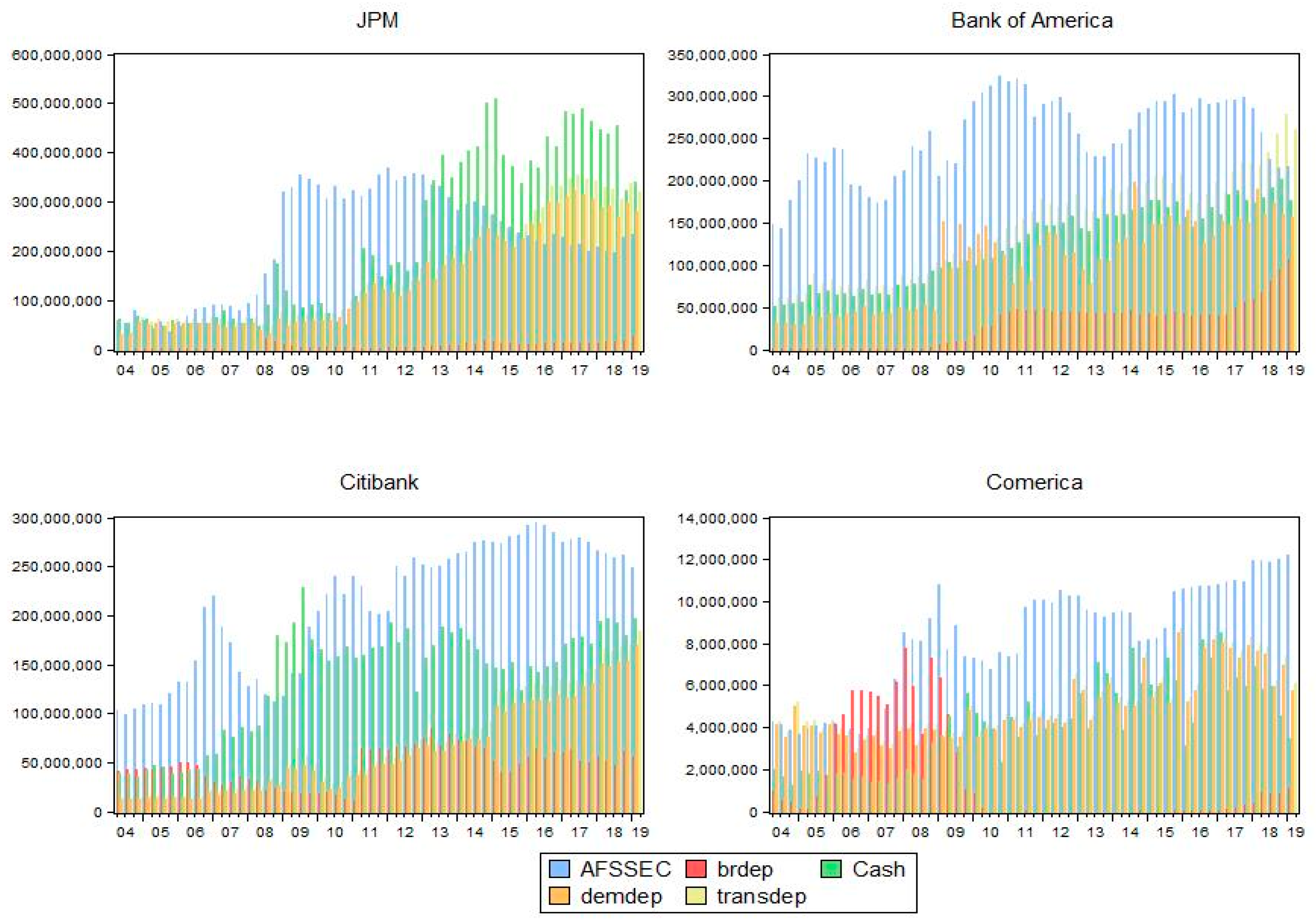
In addition to this, we employed balance-sheet data associated with the banks in our sample. The variables selected were cash (RCFD0010), available-for-sale securities, total (RCFD1773), demand deposits (RCON2210), transactions deposits (RCON2215), and brokered deposits (RCON2365). These were collected from the Compustat platform for the interval marked by 2004:1 and 2019:1 and had a quarterly frequency. We employed a data selection scheme for both banks and variables that was based on data availability and the quality of the time series. As mentioned in both the introduction and the above paragraph, our variable selection relies first of all on a theoretical consideration of market liquidity present in recent empirical works, see, for example, Wegner (2020). Besides this, at present at least, dedicated databases do not report other liquidity-related balance-sheet variables for the US banking sector. Appendix A shows the time evolution of the variables for each bank.

3.1. Marginal Expected Shortfall

Our methodology is built around two major steps. First of all, we computed the Marginal Expected Shortfall for every bank included in the sample. These estimations would be treated later in the empirical construction as an input of our regression approach. From the perspective of Acharya et al. (2010), MES is a systemic risk measure that captures the potential losses should a tail event occur on the market. MES is built on the logic that the conditional returns for a specific institution should point out any systemic event. Acharya et al. (2010) highlight the construction, predictive power, and properties from a firm-level risk management perspective, and further studies such as Löffler and Raupach (2013) demonstrate its capacity to isolate systemic relations.

In order to compute MES, the expected shortfall must be defined as:

$$E{S}_j=-E\left[E|R\le -Va{R}_j\right]$$

(1)

The contribution of a bank to the expected shortfall of the system is given by:

$$E{S}_j=-{\displaystyle \sum }_k^n{y}_{k}E\left[r_k|R\le -Va{R}_j\right]$$

(2)

where $r_k$ is the bank’s stock return, R is the group return, $y_k$ is the weighting of bank k in the system.

It follows that $ME{S}_j^k$ shows the contribution of each bank to systemic risk. Broadly put, $MES$ estimates the bank’s loss when the entire system is financially distressed:

$$ME{S}_j^k=\frac{\partial E{S}_j}{\partial y_k }=-E\left[r_k|R\le -Va{R}_j\right]$$

(3)

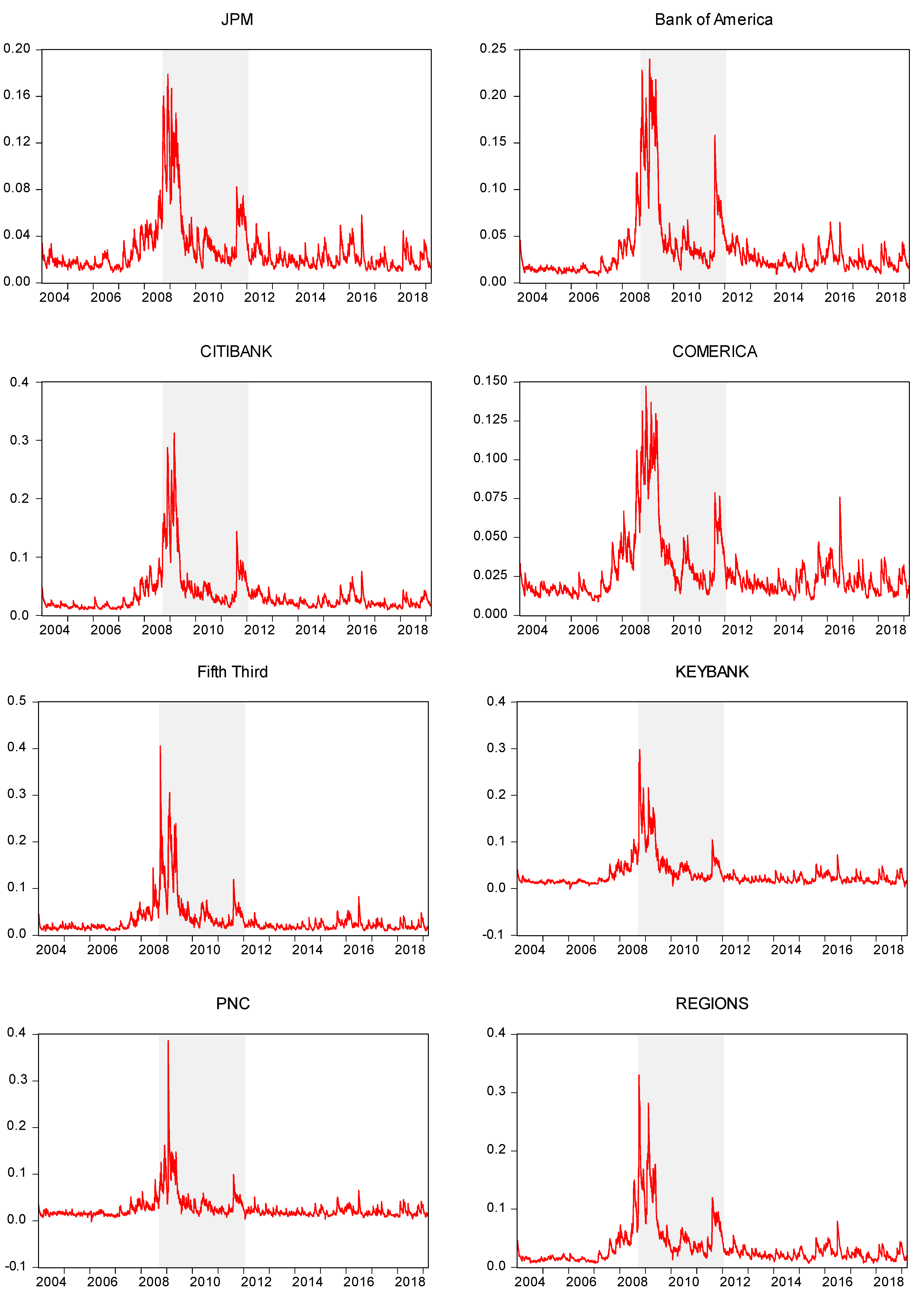
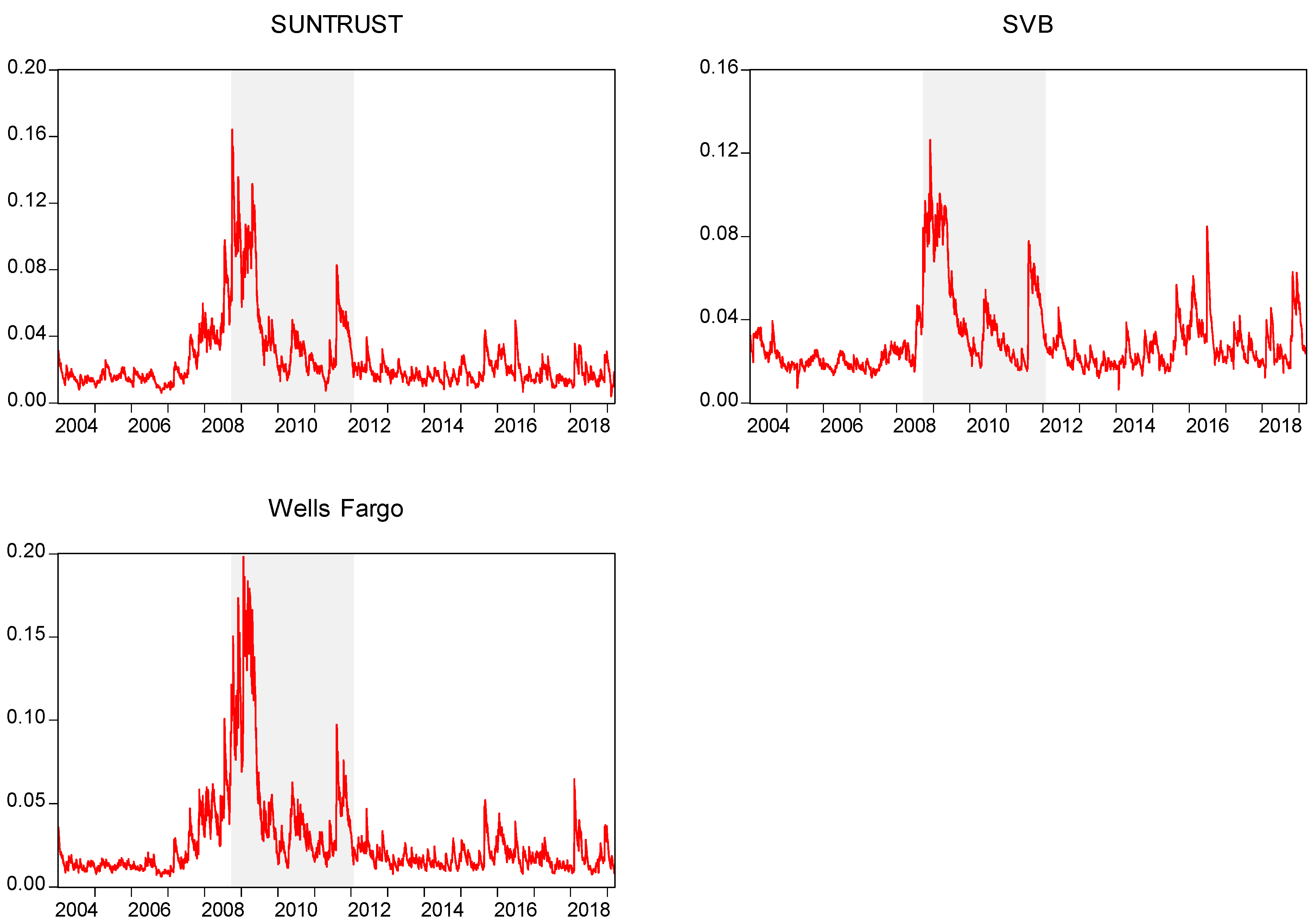
Estimations were conducted following the approach of Engle (2009). Appendix B shows a detailed analytical perspective on the dynamics of MES for the selected US Banks.

3.2. Random Forest Regression

The second step of our methodology is dedicated to our Random Forest regression procedure. As mentioned above, in this step we paired the previously obtained MES estimations for every bank in the sample with the balance-sheet liquidity proxies obtained from Compustat North America. Random Forest (hereafter RF) generates a large number of decision trees that stand as individual regression functions. Under this procedure, the result of the Random Forest regression is given by the average value of the results of all the decision trees. Breiman et al. (1984) introduce the concept of Classification and Regression Trees (CARTs), which denote nonparametric decision trees. As observed by Li et al. (2018), CARTs do not assume prior class densities, nor do they rely on a fixed tree structure. The input data determines the growth of the tree during the learning process given by a structure of decision and leaf nodes.

If we denote by Z the input vector containing m features with $Z=\left\{z_1,z_2, \cdots ,z_m\right\}$ and Y the output, $S_n$ the n-observation training set is given by:

$$S_n=\left\{(Z_1,Y_1),(Z_2,Y_2), \cdots ,(Z_n,Y_n)\right\}, Z\in {\mathbb{R}}^m,Y\in \mathbb{R}$$

(4)

In the training phase, the algorithm breaks the inputs at each node in order to optimize the parameters of the split functions so as to fit the training set. This breaking of the sample continues until a tree leaf—terminal node—is reached (Li et al. 2018).

As a consequence of the training process, a prediction function $\widehat{h}\left(Z,S_n\right)$ is formed over $S_n$.

Random Forest regressions are built on the CART specification and rely on the formation of multiple uncorrelated decision trees which are later combined via a bagging procedure. Bagging or bootstrap aggregation has been introduced by Breiman (1996) and is a valuable instrument in improving prediction performance.

The logic behind RF modeling relies on randomly incorporating a feature subset for each tree in addition to randomly considering a training data subset, again for each tree. In this setup, a bootstrap sample is formed by the randomly selecting n observations from $S_n$. As efficiently explained by Li et al. (2018), the bagging algorithm isolates various samples $\left(S_n^{{\mathsf{\Theta }}_1},\cdots , S_n^{{\mathsf{\Theta }}_q}\right)$ and deploys the above-referenced decision tree approach so as to generate a stack of q prediction trees.

$$\widehat{h}\left(X,S_n^{{\mathsf{\Theta }}_1}\right),\cdots , \widehat{h}\left(X,S_n^{{\mathsf{\Theta }}_q}\right)$$

(5)

The procedure produces q results analogous to each tree which can be expressed as:

$${\widehat{Y}}_1=\widehat{h}\left(X,S_n^{{\mathsf{\Theta }}_1}\right), {\widehat{Y}}_2=\widehat{h}\left(X,S_n^{{\mathsf{\Theta }}_2}\right), \cdots , {\widehat{Y}}_q=\widehat{h}\left(X,S_n^{{\mathsf{\Theta }}_q}\right),$$

(6)

The next step of the algorithm executes the average of the results of all trees which leads to the estimation of $\widehat{Y}.$ This is formally written as:

$$\widehat{Y}=\frac{1}{q}{\displaystyle \sum }_{l=1}^q{\widehat{Y}}_l=\frac{1}{q}{\displaystyle \sum }_{l=1}^q\widehat{h}\left(X,S_n^{{\Theta }_l}\right)$$

(7)

The Random Forest approach is built around two basic concepts: a bootstrap resampling technique and training decision trees on the samples. Both of these benefit from an extensive dataset but do not suffer from limitations on our sample of 11 banks observed for our investigation period. In addition to this, Random Forest classification and regression models have been previously confirmed to be efficient even in the case of small to medium size samples, see, for example, Shaikhina et al. (2019), Couronné et al. (2018), or Qi (2012).

4. Results

We conducted Random Forest regressions employing 1000 random decision trees in order to obtain the feature importance ranking specific to the RF methodology. Feature importance factors show how relevant a $z_i$ element is in explaining the $\widehat{Y}$ variable.

Table 1. Feature importance.

Bank	Feature Importance
JPM	AFSSEC	Brdep	Demdep	Cash	Transdep
	0.24	0.24	0.2	0.18	0.14
Bank of America	Cash	Brdep	AFSSEC	Transdep	Demdep
	0.25	0.25	0.22	0.14	0.13
Citibank	Cash	AFSSEC	Brdep	Demdep	Transdep
	0.29	0.27	0.22	0.12	0.1
Comerica	Cash	AFSSEC	Brdep	Demdep	Transdep
	0.3	0.2	0.2	0.17	0.13
Wells Fargo	Brdep	Cash	Transdep	AFSSEC	Demdep
	0.36	0.26	0.14	0.12	0.12
SunTrust	AFSSEC	Cash	Brdep	Transdep	Demdep
	0.31	0.26	0.19	0.13	0.11
Fifth Third	Brdep	AFSSEC	Cash	Transdep	Demdep
	0.34	0.24	0.18	0.13	0.11
KeyBank	Cash	Brdep	AFSSEC	Transdep	Demdep
	0.31	0.25	0.22	0.12	0.1
SVB	Cash	AFSSEC	Demdep	Transdep	-
	0.3	0.28	0.22	0.2
Regions	Cash	Brdep	AFSSEC	Demdep	Transdep
	0.29	0.2	0.19	0.19	0.12
PNC	Cash	AFSSEC	Brdep	Demdep	Transdep
	0.31	0.25	0.18	0.14	0.13

AFFSEC—Available-for-sale securities; Brdep—Brokered deposits; Demdep—Demand deposits; Transdep—Transactions deposits. Source: Author’s computation.

shows the feature importance for each bank included in our sample.

We noticed from the start that our results are rather bank-specific. This is in line with the work of Jean-Loup (2017) who also finds liquidity conditions and risks to be heterogeneous among banks. Despite this fact, several patterns are evident. Our results show that “cash” is the balance-sheet variable that is the most efficient in explaining systemic risk for the banks included in the sample. It holds the first rank in 63.6% of cases with values ranging from 25% to 31%. In addition to this, “available-for-sale securities, total” and “brokered deposits” also appear as top variables in explaining systemic risk proxied by MES, both in 18.18% of the cases. In this respect, our finding is similar to that of van den End and Tabbae (2012). They argue, like we do, that cash, readily marketable securities, as they call them, and several other types of deposits provide key insights into bank behavior and risk exposure. In a broad sense, these balance-sheet variables, although rather descriptive, convey a great amount of information and even uncover market-wide trends and forward proclivities. Available-for-sale securities are particularly relevant in what concerns fire-selling processes. Naturally, a higher share of securities available for immediate sale, decrease bank vulnerability to liquidity shocks. Greenwood et al. (2015) give an explanation of the vulnerability of banks to systemic deleveraging. More exactly, when a negative equity shock occurs, banks try to deleverage by selling assets, which further induces spillover effects. Brokered deposits, although considered riskier and allowed only for well-capitalized banks, prove to be a great source of liquidity and confidence, thus being an important feature in explaining bank risk. Cont et al. (2020) specifically demonstrate the negative impact of liquidity shortages—through the new financing costs that arise—and of fire sales on bank solvency. Our results confirm their assertions.

We notice more homogeneity for the features that are the least valuable in explaining our dependent variable, these being demand deposits and transactions deposits.

For the case of JPMorgan Chase & Co, we remarked that 24% of the systemic risk measured in our analysis by Marginal Expected Shortfall is explained by the balance-sheet position concerning the total value of available-for-sale securities. The same contribution is brought by brokered deposits (24%), while the third position is held by demand deposits. Contrary to several other cases, the systemic risk for JPMorgan Chase & Co is explained by cash only by a margin of 18%. The least significant feature is the value placed in transactions deposits.

In Bank of America’s case, cash—or the lack, thereof—drives 25% of its systemic risk, just the same as brokered deposits. Not far behind, available-for-sale securities account for 22%. Lower feature importance is attributed to transactions and demand deposits (with 14% and 13%, respectively).

The following two institutions, Citibank and Comerica, have similar rankings. Cash is the main explanatory variable for risk for Citibank with 29%, followed closely by available-for-sale securities with 27%. Brokered deposits rank third, with 22%. Transactions and demand deposits have a lower explanatory power for systemic risk (12% and 10% during the sample period). For Comerica, cash is also the most important feature (30%). Available-for-sale securities and brokered deposits have equal contributions to Marginal Expected Shortfall at 20% each. Demand (17%) and transactions deposits (13%) occupy, once again, the last positions.

Brokered deposits explain the most of Wells Fargo’s potential losses (36%). Cash is the second runner with 26%. Unlike all the other cases, available-for-sale securities do not seem to drive much of the risk. Their importance accounts for only 12%, an equal amount to demand deposits.

Similar to JPMorgan Chase & Co, SunTrust’s Marginal Expected Shortfall is partly driven by available-for-sale securities (31%) and cash (26%). Lower importance weightings are assigned to brokered deposits (19%), transactions deposits (13%), and demand deposits (11%).

For the case of Fifth Third, 34% of the potential loss is explained by brokered deposits, while available-for-sale securities contribute 24%. Surprisingly, cash is third with 18%. Transactions (13%) and demand deposits (11%) have the lowest implications on systemic risk.

Cash renders most of KeyBank’s expected loss (31%), followed by brokered deposits (25%) and available-for-sale securities (22%). Transactions deposits (12%) and demand deposits (10%) come last.

SVB is a particular case where the brokered deposits data were not available. However, we noticed similar patterns with the other banks; cash (30%) and available-for-sale securities (28%) have comparable feature importance values. A lower contribution to Marginal Expected Shortfall is given by demand deposits (22%) and transactions deposits (20%).

In the case of Regions Bank, the expected loss is influenced by cash availability in a proportion of 29%, followed by brokered deposits with 20%. An equal contribution is made by available-for-sale securities and demand deposits at 19%.

Last, but not least, PNC’s risk is explained to a great extent by cash (31%) and available-for-sale securities (25%). Brokered deposits occupy the third position (18%). Demand deposits (14%) and transactions deposits (13%) contribute to a lesser extent to systemic risk exposure.

As mentioned above, the results are heterogeneous but display specific patterns. From a broad perspective, we can confirm the connection between balance-sheet variables and systemic risk, as also argued by Idier et al. (2014), Bell and Hindmoor (2018), or Jean-Loup (2017). Moreover, we find evidence that the variability of some liquidity proxies from the balance-sheet does explain the variability of systemic risk. Out of the five exogenous variables, cash, available-for-sale securities, and brokered deposits occupy the first three places in most cases during the observed period.

5. Conclusions

The nexus between bank fundamentals and systemic risk has been addressed time and again. Naturally, balance-sheet indicators can reflect bank fragility to a great extent. This relationship is the object of theoretical models testing for balance-sheet vulnerabilities. It may be already common knowledge that bank liquidity shortages are linked with higher probabilities of bank runs (Morris and Shin 2008; Diamond and Rajan 2005; Pierret 2015). Some studies expand on this issue and find strong evidence that balance-sheet data do hint towards systemic vulnerabilities (Bell and Hindmoor 2018), or that systemic risk is higher for banks with weak balance-sheet characteristics (Idier et al. 2014).

Our investigation is motivated by the relevant role played by liquidity in systemic risk modeling for the case of the banking sector. In this paper, we aim to study the extent to which systemic risk dynamics are determined by a series of balance-sheet liquidity proxies. Our analysis focuses on a batch of US banks, observed in the 2004–2019 interval. We use as a systemic risk measure the Marginal Expected Shortfall (MES) introduced by Acharya et al. (2010) and balance-sheet elements for each bank retrieved from Compustat.

Our first relevant result is that the feature importance is bank-specific, in the sense that we obtain heterogeneous results for the main drivers of systemic risk. Nevertheless, we notice that the largest influence is rendered, in most cases, by cash, available-for-sale securities, and brokered deposits. Besides focusing on this general perspective, we also consider each bank in turn and determine both rank and percentage for each feature importance. Cash is the balance-sheet variable that is the most efficient in explaining marginal losses. Available-for-sale securities are particularly relevant in what concerns fire-selling processes. Naturally, a higher share of securities available for immediate sale decreases bank vulnerability to liquidity shocks. From this point of view, our findings are in line with Greenwood et al. (2015). Since cash and available-for-sale securities are the most liquid assets on a bank’s balance sheet, it is fairly normal for them to be volatile and to drive most of the Marginal Expected Shortfall. More recently, Bakoush et al. (2019) or Nguyen et al. (2020) also stress the importance of highly liquid instruments in avoiding systemic liquidity risk.

Our results give better insight into the link between balance-sheet liquidity proxies and systemic risk and call for the need for heightened prudential regulation of bank liquidity. This evidence-based assertion is also put forward by Tirole (2011) and Sum (2015). The findings yield some relevant implications for supervisory authorities. A point often overlooked, the straight-forward regulation of balance-sheet items as such may be a plausible prudential instrument. More exactly, imposing minimum weights for cash and immediate liquidity assets should prove useful in avoiding systemic risk build-up and liquidity runs. We must agree with van den End and Tabbae (2012) that a sufficient provision of liquid buffers could prevent shocks and spillovers. Furthermore, systemic risk and consequent systemic crises could be consistently tamed by consolidating bank emergency liquidity provision schemes.

In general terms, the present research could be extended by incorporating more balance-sheet elements that can offer information about bank liquidity. As stated before, one strong limitation of the present study derives from the lack of data available for our investigation period.

References

1. Acharya, Viral V., Lasse H. Pedersen, Thomas Philippon, and Matthew Richardson. 2010. Measuring Systemic Risk. Federal Reserve Bank of Cleveland Working Paper 2010. Available online: https://www.clevelandfed.org/en/newsroom-and-events/publications/working-papers/working-papers-archives/2010-working-papers/wp-1002-measuring-systemic-risk.aspx (accessed on 4 August 2020).
2. Adrian, Tobias, and Nina Boyarchenko. 2018. Liquidity policies and systemic risk. Journal of Financial Intermediation 35: 45–60. [Google Scholar] [CrossRef] [Green Version]
3. Adrian, T., and M. K. Brunnermeier. 2016. CoVaR. American Economic Review 106: 1705–41. [Google Scholar] [CrossRef]
4. Ahrend, Rudiger, and Antoine Goujard. 2015. Global banking, global crises? The role of the bank balance-sheet channel for the transmission of financial crises. European Economic Review 80: 253–79. [Google Scholar] [CrossRef]
5. Aldasoro, Iñaki, and Ester Faia. 2016. Systemic loops and liquidity regulation. Journal of Financial Stability 27: 1–16. [Google Scholar] [CrossRef]
6. Alessi, Lucia, and Carsten Detken. 2018. Identifying excessive credit growth and leverage. Journal of Financial Stability 35: 215–25. [Google Scholar] [CrossRef]
7. Allen, Linda, Turan G. Bali, and Yi Tang. 2012. Does systemic risk in the financial sector predict future economic downturns? The Review of Financial Studies 25: 3000–36. [Google Scholar] [CrossRef]
8. Bakoush, Mohamed, Enrico H. Gerding, and Simon Wolfe. 2019. Margin requirements and systemic liquidity risk. Journal of International Financial Markets, Institutions and Money 58: 78–95. [Google Scholar] [CrossRef] [Green Version]
9. Ballings, Michel, Dirk Van den Poel, Nathalie Hespeels, and Ruben Gryp. 2015. Evaluating multiple classifiers for stock price direction prediction. Expert Systems with Applications 42: 7046–56. [Google Scholar] [CrossRef]
10. Bănulescu, Georgiana-Denisa, and Elena-Ivona Dumitrescu. 2015. Which are the SIFIs? A Component Expected Shortfall approach to systemic risk. Journal of Banking & Finance 50: 575–88. [Google Scholar]
11. Battaglia, Francesca, and Angela Gallo. 2013. Securitization and systemic risk: An empirical investigation on Italian banks over the financial crisis. International Review of Financial Analysis 30: 274–86. [Google Scholar] [CrossRef]
12. Bell, Stephen, and Andrew Hindmoor. 2018. Are the major global banks now safer? Structural continuities and change in banking and finance since the 2008 crisis. Review of International Political Economy 25: 1–27. [Google Scholar] [CrossRef] [Green Version]
13. Ben Ameur, Hachmi, Fredj Jawadi, Wael Louhichi, and Abdoulkarim Idi Cheffou. 2017. Modeling International Stock Price Comovements with High-Frequency Data. Macroeconomic Dynamics, 1–29. [Google Scholar] [CrossRef]
14. Billio, Monica, Roberto Casarin, Michele Costola, and Andrea Pasqualini. 2016. An entropy-based early warning indicator for systemic risk. Journal of International Financial Markets, Institutions and Money 45: 42–59. [Google Scholar] [CrossRef] [Green Version]
15. Blau, Benjamin M., Tyler J. Brough, and Todd G. Griffith. 2017. Bank opacity and the efficiency of stock prices. Journal of Banking & Finance 76: 32–47. [Google Scholar]
16. Breiman, Leo. 1996. Bagging predictors. Machine learning 24: 123–40. [Google Scholar] [CrossRef] [Green Version]
17. Breiman, Leo, Joseph Friedman, Charles Stone, and Richared Olshen. 1984. Classification and Regression Trees. Boca Raton: CRC Press. [Google Scholar]
18. Brownlees, Christian, and Robert F. Engle. 2016. SRISK: A conditional capital shortfall measure of systemic risk. The Review of Financial Studies 30: 48–79. [Google Scholar] [CrossRef]
19. Buch, Claudia M., Thomas Krause, and Lena Tonzer. 2019. Drivers of systemic risk: Do national and European perspectives differ? Journal of International Money and Finance 91: 160–76. [Google Scholar] [CrossRef] [Green Version]
20. Cai, Juan-Juan, John H. J. Einmahl, Laurens de Haan, and Chen Zhou. 2015. Estimation of the marginal expected shortfall: The mean when a related variable is extreme. Journal of the Royal Statistical Society: Series B: Statistical Methodology 77: 417–42. [Google Scholar] [CrossRef] [Green Version]
21. Caporin, Massimiliano, and Paolo Santucci de Magistris. 2012. On the evaluation of marginal expected shortfall. Applied Economics Letters 19: 175–79. [Google Scholar] [CrossRef]
22. Chang, Carolyn W., Xiaodan Li, Edward M. H. Lin, and Min-The Yu. 2018. Systemic risk, interconnectedness, and non-core activities in Taiwan insurance industry. International Review of Economics & Finance 55: 273–84. [Google Scholar]
23. Cipra, Tomáš, and Radek Heyndrich. 2017. Systemic Risk in Financial Risk Regulation. Czech Journal of Economics and Finance 67: 15–38. [Google Scholar]
24. Coleman, Thomas F., Alex LaPlante, and Alexey Rubtsov. 2018. Analysis of the SRISK measure and its appli-cation to the Canadian banking and insurance industries. Annals of Finance 14: 547–70. [Google Scholar] [CrossRef]
25. Cont, Rama, Artur Kotlicki, and Laura Valderrama. 2020. Liquidity at risk: Joint stress testing of solvency and liquidity. Journal of Banking & Finance 118: 105871. [Google Scholar]
26. Couronné, Raphael, Philipp Probst, and Anne-Laure Boulesteix. 2018. Random forest versus logistic regression: A large-scale benchmark experiment. BMC Bioinformatics 19: 270. [Google Scholar] [CrossRef] [PubMed]
27. Diamond, Douglas W., and Raghuram G. Rajan. 2005. Liquidity shortages and banking crises. Journal of Finance 60: 615–47. [Google Scholar] [CrossRef] [Green Version]
28. van den End, Jan Willem, and Mostafa Tabbae. 2012. When liquidity risk becomes a systemic issue: Empirical evidence of bank behaviour. Journal of Financial Stability 8: 107–20. [Google Scholar]
29. Engle, Robert. 2009. Anticipating Correlations: A New Paradigm for Risk Management. Princeton: Princeton University Press. [Google Scholar]
30. Engle, Robert, Eric Jondeau, and Michael Rockinger. 2014. Systemic Risk in Europe. Review of Finance 19: 145–90. [Google Scholar] [CrossRef]
31. Greenwood, Robin, Augustin Landier, and David Thesmar. 2015. Vulnerable banks. Journal of Financial Economics 115: 471–85. [Google Scholar] [CrossRef]
32. Grundke, Peter, and Michael Tuchscherer. 2018. Global systemic risk measures and their forecasting power for systemic events. The European Journal of Finance 25: 1–29. [Google Scholar] [CrossRef]
33. Hautsch, Nikolaus, Julia Schaumburg, and Melanie Schienle. 2015. Financial network systemic risk contributions. Review of Finance 19: 685–738. [Google Scholar] [CrossRef] [Green Version]
34. Idier, Julien, Gildas Lamé, and Jean-Stéphane Mésonnier. 2014. How useful is the Marginal Expected Shortfall for the measurement of systemic exposure? A practical assessment. Journal of Banking & Finance 47: 134–46. [Google Scholar]
35. Jabeur, Sami Ben, and Youssef Fahmi. 2018. Forecasting financial distress for French firms: A comparative study. Empirical Economics 54: 1173–86. [Google Scholar] [CrossRef]
36. Jean-Loup, Soula. 2017. Measuring heterogeneity in bank liquidity risk: Who are the winners and losers? The Quarterly Review of Economics and Finance 66: 302–13. [Google Scholar] [CrossRef] [Green Version]
37. Kleinow, Jacob, Fernando Moreira, Sascha Strobl, and Sami Vähämaa. 2017. Measuring systemic risk: A comparison of alternative market-based approaches. Finance Research Letters 21: 40–46. [Google Scholar] [CrossRef] [Green Version]
38. Li, Yi, Changfu Zou, Maitane Berecibar, Elise Nanini-Maury, Jonathan C. W. Chan, Peter van den Bossche, Joeri Van Mierlo, and Noshin Omar. 2018. Random forest regression for online capacity estimation of lithium-ion batteries. Applied Energy 232: 197–210. [Google Scholar] [CrossRef]
39. Lin, Edward MH, Edward W. Sun, and Min-Teh Yu. 2018. Systemic risk, financial markets, and performance of financial institutions. Annals of Operations Research 262: 579–603. [Google Scholar]
40. Löffler, Gunter, and Peter Raupach. 2013. Robustness and Informativeness of Systemic Risk Measures. Deutsche Bundesbank Research Centre, Discussion Papers 04/2013. Available online: https://www.econstor.eu/bitstream/10419/70922/1/739429647.pdf (accessed on 4 August 2020).
41. Morris, Stephen, and Hyun Song Shin. 2008. Financial regulation in a system context. Brookings Papers on Economic Activity 2008: 229–61. [Google Scholar] [CrossRef] [Green Version]
42. Nguyen, Thach Vu Hong, Shamim Ahmed, Thanaset Chevapatrakul, and Enrico Onali. 2020. Do stress tests affect bank liquidity creation? Journal of Corporate Finance 64: 101622. [Google Scholar] [CrossRef]
43. Pederzoli, Chiara, and Costanza Torricelli. 2017. Systemic risk measures and macroprudential stress tests: An assessment over the 2014 EBA exercise. Annals of Finance 13: 237–51. [Google Scholar] [CrossRef]
44. Pierret, Diane. 2015. Systemic Risk and the Solvency-Liquidity Nexus of Banks. International Journal of Central Banking 11: 193–227. [Google Scholar] [CrossRef] [Green Version]
45. Qi, Yanjun. 2012. Random forest for bioinformatics. In Ensemble Machine Learning. Boston: Springer, pp. 307–23. [Google Scholar]
46. Schuermann, Til. 2014. Stress testing banks. International Journal of Forecasting 30: 717–28. [Google Scholar] [CrossRef]
47. Shaikhina, Torgyn, Dave Lowe, Sunil Daga, David Briggs, Robert Higgins, and Natasha Khovanova. 2019. Decision tree and random forest models for outcome prediction in antibody incompatible kidney transplantation. Biomedical Signal Processing and Control 52: 456–62. [Google Scholar] [CrossRef]
48. Sum, Katarzyna. 2015. Basic indicators of systemic risk in the EU banking sector. Implications for banking regulation. International Journal of Management and Economics 47: 36–55. [Google Scholar] [CrossRef] [Green Version]
49. Tanaka, Katsuyuki, Takuji Kinkyo, and Shigeyuki Hamori. 2016. Random forests-based early warning system for bank failures. Economics Letters 148: 118–21. [Google Scholar] [CrossRef]
50. Tirole, Jean. 2011. Illiquidity and all its friends. Journal of Economic Literature 49: 287–325. [Google Scholar] [CrossRef] [Green Version]
51. Wegner, Danilo Lopomo Beteto. 2020. Liquidity policies and financial fragility. International Review of Economics & Finance. In press, Journal Pre-Proof. [Google Scholar]
1
JP Morgan Chase, Bank of America, Citibank, Comerica, Wells Fargo, SunTrust, Fifth Third, SVB, Regions, and PNC.