Article

Understanding the Accuracy Limitations of Quantifying Methane Emissions Using Other Test Method 33A

1
Department of Mechanical and Aerospace Engineering, Statler College of Engineering, West Virginia University, Morgantown, WV 26505, USA
2
Wadsworth Department of Civil and Environmental Engineering, Statler College of Engineering, West Virginia University, Morgantown, WV 26505, USA
*
Author to whom correspondence should be addressed.
Environments 2022, 9(4), 47; https://doi.org/10.3390/environments9040047
Submission received: 3 March 2022 / Revised: 22 March 2022 / Accepted: 31 March 2022 / Published: 6 April 2022

Abstract

:
Researchers have utilized Other Test Method (OTM) 33A to quantify methane emissions from natural gas infrastructure. Historically, errors have been reported based on a population of measurements compared to known controlled releases of methane. These errors have been reported as 2σ errors of ±70%. However, little research has been performed on the minimum attainable uncertainty of any one measurement. We present two methods of uncertainty estimation. The first was the measurement uncertainty of the state-of-the-art equipment, which was determined to be ±3.8% of the estimate. This was determined from bootstrapped measurements compared to controlled releases. The second approach of uncertainty estimation was a modified Hollinger and Richardson (H&R) method which was developed for quantifying the uncertainty of eddy covariance measurements. Using a modified version of this method applied to OTM 33A measurements, it was determined that uncertainty of any given measurement was ±17%. Combining measurement uncertainty with that of stochasticity produced a total minimum uncertainty of 17.4%. Due to the current nature of stationary single-sensor measurements and the stochasticity of atmospheric data, such uncertainties will always be present. This is critical in understanding the transport of methane emissions and indirect measurements obtained from the natural gas industry.

1. Introduction

An improved understanding of anthropogenic methane emissions from natural gas infrastructure is important as recent studies continue to show that current inventories underestimate methane emissions [1,2]. Uncertainty has been a major concern with respect to the indirect quantification of methane emissions. Top-down and bottom-up studies have historically resulted in large differences due to uncertainties associated with the propagation of estimates and measurement techniques, and research continues to focus on reconciling these divergent estimates [3]. Many new technologies have been developed to identify elevated methane emissions and many are focused on indirect quantification or single sensor point measurements [4]. Some indirect quantification methods focused on gas dispersion and downwind measurements from sites, but still require site access for the release of tracer gases [5,6,7]. In this work, we utilized different methods to determine the minimum uncertainty associated with a single-sensor indirect methane quantification method that does not require direct site access, can be completed at the fence line or beyond, and does not require the use of tracer releases. The method evaluated, which has been widely used by researchers and agencies to quantify methane emissions indirectly, was Other Test Method (OTM) 33A [8,9,10,11,12,13]. The Environmental Protection Agency (EPA) began development of the OTM 33 series in 2006 to focus on three primary areas: concentration mapping, source characterization, and emissions quantification. Here, we focus on the emissions quantification portion of OTM 33A, which will subsequently be referred to as OTM. The method was designed to target methane emissions from the natural gas infrastructure from sources that were near ground level, relatively small in source area, and within 150 m (m) of the measurement location [8]. The method produces a mass emission rate by utilizing a point source Gaussian methodology to measure a horizontal flux. OTM was recently compared with tracer methods and direct quantification techniques and tended to underpredict emissions, but it was noted to be a quick and non-invasive method to estimate emissions [7]. An additional benefit of the OTM approach is that its equipment can also be vehicle mounted to enable a slightly different method for mobile sensing [14,15,16]. Details on the OTM method have been extensively explained elsewhere [9,10,11,12,13]. To reduce the uncertainty of the method, a series of Data Quality Indicators (DQI) were developed. Multiple studies have been conducted on the accuracy of OTM with controlled release experiments. The initial releases, performed by the EPA, took place alongside the development of the method, and were used in development of the DQIs and detailed in Brantley et al. [9]. These tests consisted of 107 observations each spanning approximately 15–20 min. The method produced an initial accuracy which ranged from −84% to 184%. After eliminating periods of data that did not meet the primary DQIs, 74% remained. The errors of these measurements ranged from −60% to 52%; however, 71% of measurements were within ±30% of the actual release rate [13].
Robertson et al. performed a second series of controlled release experiments at Christman Airfield (CAF) in Fort Collins, CO for comparison with those performed by Brantley et al. [9,12]. This series of experiments consisted of 23 tests. Four of the measurements were eliminated from analysis because they did not pass one of the three primary DQIs. Robertson et al. combined these results with those from Brantley et al., which resulted in a dataset of 119 tests. These data had a 2σ error of ±56% and a 1σ error of ±28%. Robertson et al. reported a 10% low bias but noted that the Brantley et al. data did not share this bias [12].
A recent study by Edie et al. further investigated the controlled release experiments of Robertson et al. and performed a third set of controlled releases at the Methane Emissions Technology Evaluation Center (METEC), also in Fort Collins [12]. The study observed that across each test set the wind speed, number of sources, and leak height had no major impact on estimate accuracy. This research analyzed 34 total tests, 24 of which passed the DQI threshold. The total error range was −60% to +170% with a 68th percentile of error at ±38%. An ordinary least squares regression analysis confirmed the 10% low bias seen by Robertson et al. and a propensity to overestimate smaller releases. The study concluded that OTM measurements could generally expect a 2σ error of ±70% with a slight negative bias. A summary of the previously performed controlled release experiments and their resultant uncertainties is presented in the Materials and Methods section.
As presented, the uncertainty associated with the method can be large for a population of measurements. This means that the uncertainty of any individual measurement may be even more significant. Currently, the use of DQIs as a quality assurance is the most effective way to ensure an accurate measurement is performed. This method by no means guarantees any level of accuracy. Repeat measurements can increase the confidence of measurements. However, the stochastic nature of micrometeorological conditions makes such measurements difficult to obtain. Methods need to be explored to determine the minimum uncertainty of a given measurement based on the measurement principle itself.
We investigated the minimum obtainable uncertainty associated with the use of the OTM method. State-of-the-art equipment was utilized in a configuration commonly used for a method known as Eddy Covariance (EC). The EC method is generally used to measure vertical fluxes from homogenous emission sources; however, it relies on much of the same instrumentation as OTM. Methods were used in tandem during this research effort. The results from the combination of methods are presented in a concurrent publication [17]. Here, we focus on the uncertainty associated with the OTM method from the perspective of both minimum measurement error due to equipment specifications and the variability in measurements by utilizing an uncertainty technique common to the EC research community. This methodology, developed by Hollinger and Richardson (H&R) [18], was modified to quantify the measurement-to-measurement variability of the OTM method.

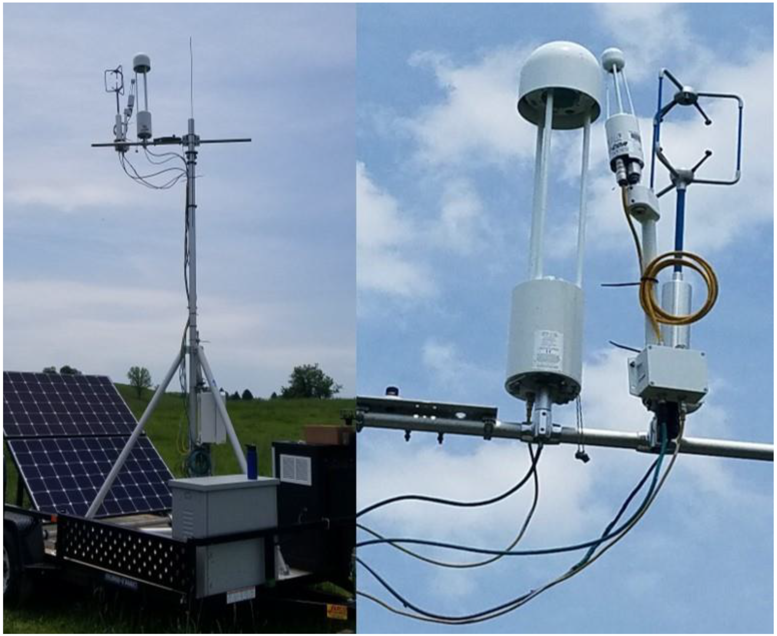
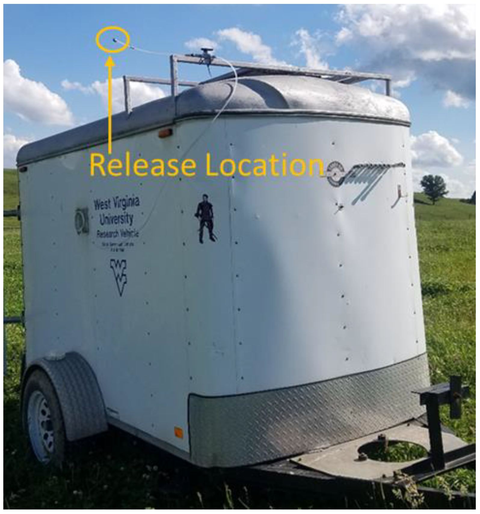
2. Materials and Methods

The primary method of data acquisition (DAQ) was an in-house developed Mobile Eddy Covariance Tower (MECT). The design of this DAQ system was specific to this research, as it was intended to be semi-mobile for easy movement and deployment. The tower was mounted on a towable trailer so that it could easily be moved within and among natural gas production sites. The MECT was designed for operation without an external power source. The DAQ equipment mounted on the tower was powered by a rechargeable battery bank which was maintained by two solar panels, also mounted on the trailer. This system could be transported and deployed at different sites as a single system with relative ease compared to conventional EC stationary systems. The DAQ system included a LICOR LI-7700 CH4 analyzer, LI-7500DS CO2/H2O analyzer, LI-200R pyranometer (Lincoln, NE, USA), a Gill® WindMaster 3-axis sonic anemometer (Lymington, UK), and an Omega iBTHx barometric pressure, temperature, and humidity sensor (Norwalk, CT, USA) [19,20,21,22,23]. Data from the system were recorded at a rate of 10 Hz. The LI-7700, LI-7500, and WindMaster were mounted vertically, 4 m from the base of the trailer. The trailer base was about 0.5 m above the ground; therefore, the sensor height was considered 4.5 m for data processing. Details of the DAQ system can be found in [11,24]. More details on the DAQ equipment specifications are presented in the Appendix A, Table A1. The DAQ setup is presented in Figure A1.
The initial deployment of the MECT for controlled release experiments occurred at the WVU JW Ruby Research Farm located in Reedsville, WV [25]. This site was used in this research due to its open fields which contained no high canopy vegetation or building interference, similar to conditions at well sites. Two open fields served as locations for experiments involving controlled releases of methane. These fields were normally used for cattle grazing; however, no cattle were present in the fields while they were used for experiments. It should be noted that at times the cattle were in adjacent fields and could have contributed to elevated background methane concentrations in the area. The MECT was deployed and collected data continuously during the controlled releases performed at the farm.
The controlled release experiments were designed based on previous OTM studies and directly quantified emissions from a local production site [26,27,28]. The designed release/distance matrix consisted of nine different release rate/distance (RRD) scenarios. Methane release rates ranged from 0.04 to 0.24 grams per second (g/s). Distances ranged from 40 to 120 m. The distances were approximated with a range finder and later calculated based on the GPS coordinates of the release point and the data collection point (the MECT location). The final controlled release matrix is presented in Table A2.
The controlled releases were produced from a three-bottle, pressure-controlled manifold of technical to high purity methane (98–99% composition by volume) connected in parallel to a mass flow controller. The release point was attached to the roof of the trailer at a height of approximately 2.3 m. The methane was released from this point at atmospheric pressure, simulating a release from an onsite blunt body, such as a tank. The release setup is presented in Figure A2.
Data collection occurred between 21 May and 11 September 2019. Information on initial data elimination can be found in [11]. The data used for this research were based on those averaging periods that produced valid results from both OTM and EC calculations. Averaging periods were 15 min in length to allow for the alignment of EC and OTM data and only those periods with an average prevailing wind direction within ±45° of the source to sensor (StS) direction were utilized.
During the entire farm deployment there were a possible 10,878 15 min periods. Of those, 7283 (67%) resulted in valid OTM and EC calculations. Of those 7283 valid OTM estimations, 4599 (63%) were from periods without a release present and 2684 (37%) were from periods with a release. Of the 2684 valid periods during controlled release periods, 804 (30%) were within ±45° of the StS direction. Of the 4459 valid background periods, 3124 (68%) occurred after the first controlled release was initiated. Of these 3124 periods, 1208 (39%) of them were within ±45° of the StS direction. These were considered the final background periods and were used for further analysis. The final available dataset consisted of 15 min periods recorded after the first release was initiated, with valid OTM and EC estimates and had an average wind direction within ±45° of the StS direction. The final number of background periods with these properties was 1208 and the final number of controlled release periods with these properties was 804. The valid periods broken down by distance and release rate are presented in Table 1.
Wind speed was considered one of the most critical variables for the success of various indirect quantification techniques. The average 15 min period mean wind speed was 1.6 m/s and the maximum was 5.3 m/s. This aligns with the recommendation of Robertson et al. that OTM measurements were most effective with average wind speeds of 1 to 10 m/s. The controlled releases of Robertson et al. experienced atmospheric stability indicator (ASI) values between 2–6 [12]. The ASI is a measure of atmospheric stability and aligns closely with the widely used Pasquill stability classes [9]. Edie et al. performed controlled release experiments with wind speeds between 2–8 m/s and ASI values between 3–6 [10]. The ASI values of this work varied between 2–7 but tended to be higher with a mean value of 5, which suggested that conditions tended to be more stable.
For comparison with the results of other research, the periods in this dataset with a low DQI were examined as a population. There were 181 averaging periods with a DQI below 10 based the criteria defined by Edie et al. [10]. The 1σ error of these periods was ±61%, which was closer to the 2σ errors reported by previous studies. One of the reasons was likely the larger number of sample periods which allowed for more potential that there would be a large outlier in the set. Another cause may have been that previous research tended to be performed in more favorable conditions for OTM. A complete comparison of the population of errors for those tests with a DQI less than ten is presented in Table 2. Data for the 181 averaging periods with a DQI less than ten are provided as Supplementary Materials.
These uncertainties are only for populations of data. The goal of this work was to determine the minimum achievable uncertainty of such methods. Currently, significant efforts are being made to reduce the uncertainty of indirect measurements in the field of methane quantification. However, instrumentation and stochasticity are likely to limit the potential improvements that can be made by more advanced methods. Understanding the limitations on uncertainty could enable better assessment of future modifications made to indirect techniques similar to OTM 33A.

3. Results and Discussion

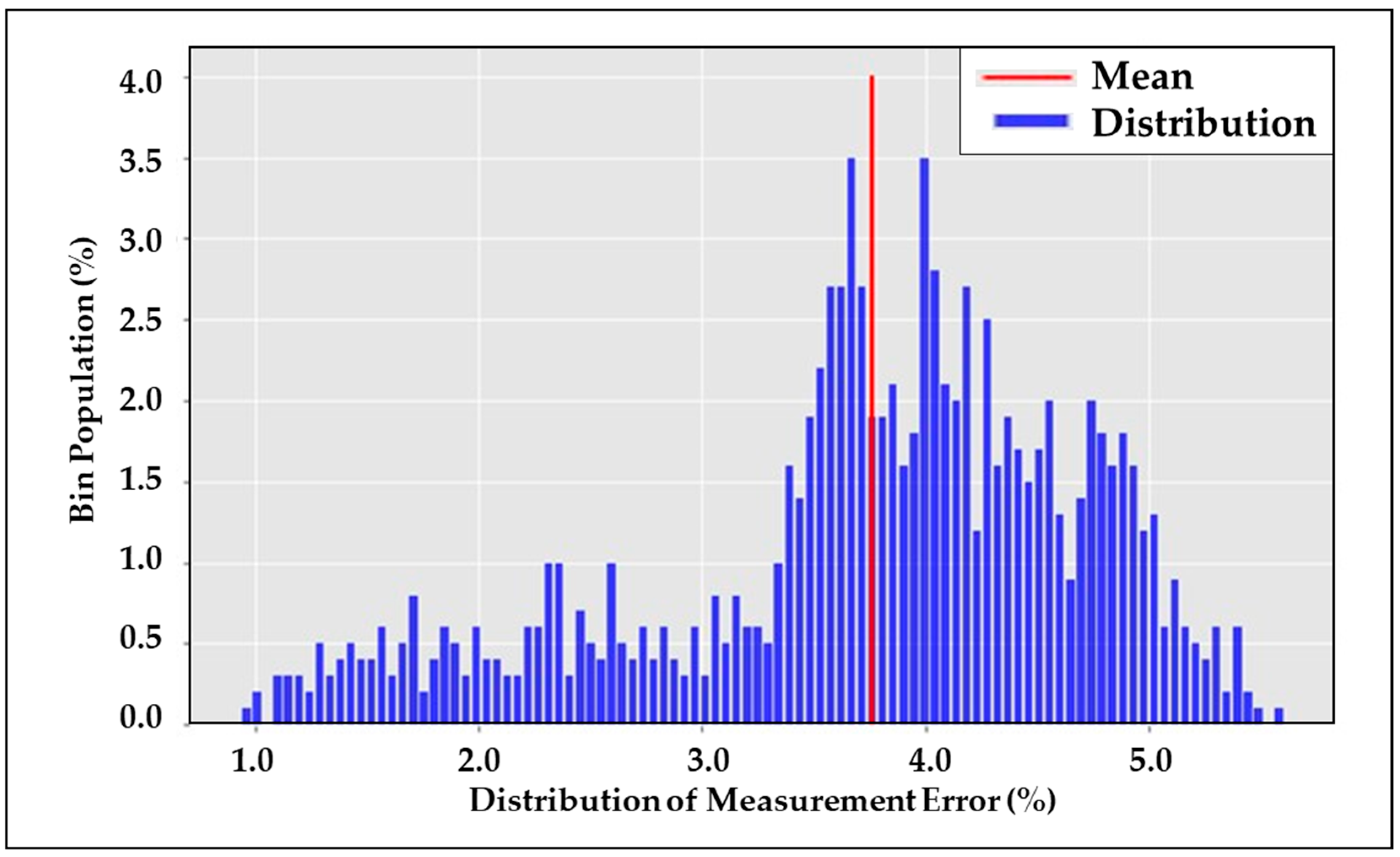
3.1. Instrument Uncertainty

The key variables used for OTM calculations were 3-D wind speeds, methane concentration, temperature, and pressure. The instruments used to measure these variables and their respective uncertainties are presented in Table 3.
The uncertainty of each instrument measurements was determined by combining the uncertainties associated with resolution and accuracy. The uncertainty of each individual data point collected at 10 Hz were determined for each of the respective instruments. The accuracy uncertainty was determined based on the interval within which the true value was known. If the accuracy of a device was presented as a percentage of the measurement, the actual value was assumed to fall within the range of the [measured value +/− the reported accuracy (%) multiplied by the measured value]. If the accuracy was presented as an engineering unit, the actual value was assumed to fall within the range of the [measured value +/− the unit value].
Regardless of how the accuracy was reported by the device manufacturer, the standard uncertainty due to accuracy was calculated as the half interval divided by the square root of three. This calculation was derived from the assumption that the accuracy of the device acts as a rectangular distribution. In other words, all possible values within the accuracy range are equally likely for each measurement point [29]. Examples of the individual measurement uncertainties due to accuracy are presented in Calculation A1 for methane (as a percentage) and temperature (as a unit value).
The instruments used for measurement also had uncertainties associated with their resolution. Since any digital instrument has a discrete value due to rounding, the true value could lie within ±0.5 multiples of the displayed value. To determine the standard resolution uncertainty of the device, the reported resolution was divided by the square root of three (again assuming that each possible value in the half interval were equally likely to occur) [30]. As an example, the resolution of the WindMaster is presented in Calculation A2.
The total standard uncertainty of each individual measurement could be calculated by combining the uncertainties due to resolution and accuracy [31]. The total standard uncertainty of each individual measurement point was calculated using Equation (1) for each variable.
ε   t o t a l = ε r e s o l u t i o n 2 + ε a c c u r a c y 2
A complete example of the total standard uncertainty in a measured methane concentration is presented in Calculation A3.
To determine the standard measurement uncertainty of an OTM averaging period, the total standard uncertainty of each measurement from each device was calculated. So, for each individual point (10 Hz data) the uncertainty of that measurement point was quantified. This resulted in an “upper”, “lower”, and “measured” value for each variable and each data point. There were six 10 Hz variables used in the OTM calculation (ch4, u, v, w, t, p). The three potential values of each variable are described below:
  • measured value = the value reported and recorded form the instrument
  • upper value = measured value + standard uncertainty of measured value
  • lower value = measured value − standard uncertainty of measured value
To analyze the uncertainty of an OTM averaging period estimate, a complete analysis of all the combinations of maximum measurement uncertainty were applied to each point in that period. Within a given 15 min period there were 9000 data points which could exhibit the full spectrum of measurement uncertainty. For simplicity it was assumed that the true value of every point of a given variable was either the “upper”, “lower”, or “measured” value. Applying this simplifying assumption to all six variables gave a total of 729 potential OTM estimates for each period based on the number of variables (m = 6) and number of potential values (n = 3), such that: n m = 3 6 = 729 .
For example, one of the estimates was calculated using the “upper” value for all ch4, u, and w measurements, the “lower” value for all v and t measurements, and the “measured” value for all p measurements. So, for each period 729 estimates were calculated using the OTM method and the different possible values of each variable. This produced an average and standard deviation of estimates for each period as a percentage of the actual estimate. The actual estimate was that which utilized the measured value for each of the variables.
From the 804 valid release periods, 100 random samples were selected. All 729 combinations were used to estimate mass emissions rates from these 100 periods. Measurement uncertainty as a percentage of the actual estimate was inferred from these 100 periods. The result from each combination of variables was quantified as a percentage of the measured estimate. The measurement uncertainty as percentage of the estimate was determined using the following methodology:
  • The percentage of the measured estimate was calculated for each of the 729 results for each period.
  • From these 729 results, a single estimate was randomly selected 100 times to represent the given period.
  • The mean, standard deviation (σ), and standard error (SE) of these periods were calculated. The SE was calculated using Equation (2), where n represents the number of samples (100).
  • The measurement uncertainty of the 100 samples was calculated as [±1.96 * SE] representing the 95% confidence interval (CI) of the standard normal distribution.
  • This process was repeated for 1000 iterations and the average measurement uncertainty was determined to be the measurement uncertainty for all estimates.
S E = σ n

3.2. Method Uncertainty

As stated, this project also focused on combining EC with OTM. Therefore, the data analyzed here were those averaging periods capable of producing both valid EC and OTM results. EC uncertainty methods were applied to these averaging periods. A widely used method of uncertainty estimation for EC fluxes is that of Hollinger and Richardson (H&R) [18]. The method allowed two options for quantifying flux uncertainty by quantifying the differences in measurements from periods that should produce similar results based on atmospheric drivers. One option was to utilize multiple towers to measure the same area and the other was to use a single tower measuring the same area at different times with similar conditions. The option involving only one tower utilized pairs of data measured exactly 24 h apart to reduce diurnal variability. To ensure that the periods of comparison were sufficiently similar, several qualifiers were utilized to govern accepted pairs. The original research was focused on differences in heat, water vapor, and CO2 fluxes. The qualifiers for acceptable periods were based on the drivers of these types of fluxes. The qualifiers for similar periods were defined as follows:
-
Photosynthetic Photon Flux Density (PPFD) difference less than 75 µmol/m2s
-
Air Temperature Difference less than 3 °C
-
Vapor Pressure Deficit Difference less than 200 Pa (0.2 kPa)
-
Wind Speed Difference less than 1 m/s
When two periods separated by 24 h met all defined criteria they were accepted for use in the calculation to determine the standard deviation of the measurement error [σ(δq)] as defined by H&R. The standard deviation of the measurement uncertainty can be calculated from the accepted 24 h periods with Equation (3).
σ ( δ q ) = σ ( x 1 , t x 2 , t ) 2
where σ ( δ q ) is the standard deviation of the measurement uncertainty, x 1 , t and x 2 , t are flux measurements taken 24 h apart which meet the defined criteria and σ ( x 1 , t x 2 , t ) is the standard deviation of the differences of those respective pairs. The derivation of σ ( δ q ) follows the logic that two periods with measured fluxes of x1 and x2 have measurement uncertainties associated with them of δq1 and δq2. Because the expected difference between x1 and x2 of sufficiently similar periods would be zero, it follows that the variance of (δq1 − δq2) would be equivalent to the variance of (x1x2). Hence, the standard deviation of the uncertainty was inferred from the standard deviation of the measurements whose expected values are equivalent [18]. We applied the same logic to OTM estimates. Sufficiently similar periods of measurement should yield similar results.
To quantify the uncertainty of measurements from the MECT at the farm, background (no release present) periods were used because it was expected that they would have the same value 24 h apart. Periods with controlled releases of the same rate and distance spaced 24 h apart were rare and variations in wind direction would greatly impact the estimations of these periods. The primary driver of the OTM background estimations was the natural methane flux from the soil. Yamulki et al., determined that the primary drivers of methane flux from soils in which grazing animals were sometimes active were ambient temperature and rainfall [32]. To determine the natural difference in methane flux, the qualifiers for acceptable periods were defined as follows:
-
No precipitation between periods
-
Air Temperature difference less than 3 °C
OTM relies on stability class assumptions and the estimates obtained from it are a direct product of the wind speed. Many methods of estimating stability class utilize solar loading or cloud cover in their classification [33,34]. Here, PPFD was utilized instead of solar loading or cloud cover since it provides the same information and H&R defined criteria for sufficiently similar periods. Therefore, in addition to the natural methane flux drivers, for OTM periods to be accepted they were required to meet the following additional criteria which were also defined by H&R:
-
PPFD difference less than 75 µmol/m2s
-
Wind speed difference less than 1 m/s
PPFD [µmol/m2s] is a measure of light intensity approximately equal to 4.6 W/m2 [23]. In this research the variable of solar loading in W/m2 was recorded by a pyranometer and converted to PPFD. From the background periods collected in between controlled releases there were 1208 periods that contained both valid OTM and EC estimates. From these 1208 periods there were 65 pairs of periods that met the criteria for OTM.
The goal was to determine the uncertainty from this method as a percentage of the OTM estimate, so that it could be compared with the measurement uncertainty. To determine the uncertainty as a percentage of the estimate a bootstrap of 1000 iterations on the 65 pairs was performed. For each of the iterations a sample size of 65 pairs was selected with replacement. The absolute mean of the estimates, the mean difference of the pairs, the standard deviation of measurement uncertainty, and the SE of the measurement uncertainty were calculated for each iteration. The SE was calculated as presented in Equation (2). We again used the assumption that [±1.96 * SE] was the 95% CI of the uncertainty, as was performed for the measurement uncertainty.

3.3. Instrument Uncertainy Results

The OTM measurement uncertainty due to instrument error was determined from a bootstrapped sample of 100 random periods during controlled releases. The 1000 iterations of measurement uncertainty as a percentage of the estimate are presented in Figure 1. The final measurement uncertainty of OTM estimates due to instrumentation alone was determined to be ±3.8% of the “measured” value. We see that this is similar to direct quantification measurement uncertainties for state-of-the-art systems [24,25,26,27]. Some recent research has examined low-cost sensors that could be deployed at sites to conduct measurements similar to ours. While reducing costs is important to ensure widespread implementation, our results suggest that current state-of-the-art sensors are accurate enough given the range of emissions typical at well sites. The predominant limiting factor in the method uncertainty is discussed below.

3.4. Method Uncertainy Results

In addition to the measurement uncertainty due to devices, the uncertainty due to the variability of estimates during similar micrometeorological conditions was quantified via a modified version of the H&R method traditionally used for EC uncertainty [18]. The H&R method had not previously been used for OTM estimation. OTM was designed around a Gaussian dispersion methodology which aimed to measure a horizontal flux from a target source. The same comparative logic was applied in that periods with similar methane emissions and similar atmospheric conditions should produce similar results. The modified H&R method was then used to determine the uncertainty in OTM measurements since the differences between periods with no emissions also had an expected difference of zero. To account for the distance variable in the OTM calculations, the OTM estimates for each pair of periods were calculated using each of the controlled release distances. This resulted in an increase in the magnitude of the estimate and an increase in the uncertainty with distance. The uncertainty as a percentage of the estimate, however, was linear with the increase in distance. This was because the OTM estimates were a near linear function with respect to StS distance. During the background periods, no controlled release was present. The resultant uncertainty therefore was the uncertainty in the measurement method to do lack of repeatability, rather than difference in wind direction, controlled release rate, or atmospheric stability. The mean results of the 1000 iterations are presented in Table 4. We see that the method uncertainty from the modified H&R method is ±17% compared to only ±3.8% for the measurement uncertainty. Thus, application of OTM 33A is more so limited by the stochastic micrometeorological conditions rather than limitations from measurement equipment.
The uncertainty methods and results are summarized in Table 5. For a final uncertainty estimation of OTM measurements the combined uncertainties of the instrument error and measurement variance of the modified H&R were combined using the sum of squares. The instrument error had a minimal effect on the estimated measurement uncertainty and the combined uncertainty was ±17%.
This uncertainty estimate was smaller than previously reported 1σ errors of ±28% and ±38%. The uncertainty presented here is the uncertainty associated with the measurement itself (i.e., the estimated value should be considered to have error bars of ±17.4%). This likely represents the absolute minimum uncertainty attainable and would never truly be achieved but may serve as a lower bound to target for any future modifications of OTM 33A. This minimal uncertainty definition helps to guide users of the current method and future methods. This value serves as a corollary to the use of the 1st and 2nd Law efficiencies in thermodynamics, where it makes little since to compare the 1st Law efficiency to 100% since it cannot be achieved, whereas comparing it to the best case of the 2nd Law efficiency helps realistically understand how well current systems perform. It makes little sense to compare indirect OTM 33A uncertainties to 0% or even just the measurement uncertainty of ±3.8% since the methods uncertainty is dominated by stochastic variances. In the case of Robertson et al., their 1σ error was likely approaching the minimum uncertainty attainable with OTM 33A, though a similar measurement uncertainty analysis should be considered.

4. Conclusions

Most of the research on the uncertainty and error of OTM 33A has focused on the error distribution of a population of measurements. This error can be large for a population of measurements, and our data show that uncertainty of any individual measurement may be even more significant. There is limited published research on the repeatability of the method or the baseline measurement error. Here, we have presented a methodology to estimate the baseline measurement error due to instrumentation and atmospheric stochasticity. These methods were used to determine the minimal attainable uncertainty under near perfectly repeatable conditions using state-of-the-art measurements. With state-of-the-art DAQ instrumentation, the average uncertainty due to measurement limitations was determined to be ±3.8% of the reported measurement. This value was obtained using a non-parametric bootstrap of randomly selected averaging periods collected during controlled release experiments. Only further improvement in instrument technology could further reduce already relatively low measurement errors.
A second measure of uncertainty was associated with stochastic measurements. A method developed by H&R for estimating EC uncertainty was modified for use with OTM 33A averaging periods. The method attempted to quantify the randomness of measurements by comparing averaging periods with similar environmental drivers. It would be expected that such periods would produce similar estimates. This method was utilized to estimate the OTM uncertainty due to the randomness of micrometeorological variables even when critical drivers were similar (precipitation between periods, air temperature, wind speed, solar loading, and therefore ASI). Such uncertainty will always be present in real-world measurements and represent a lack of repeatability. The uncertainty from this method was ±17% of the reported measurement, on average, across all measured distances. The combination of these two uncertainties resulted in a minimum obtainable uncertainty of ±17.4% for an individual measurement.
While some uncertainty, such as the measurement uncertainty due to the instrument limitations, will never be overcome, other forms of uncertainty could be reduced with different methods. The modified H&R uncertainty was based on the difference in measurements which should be similar. Similar modifications to the method as those applied here could benefit both EC and other indirect quantification methods given more long-term data were available to verify results. Such efforts could make it possible to better quantify differences in real-time to reduce errors. Novel machine learning methodologies could help to identify trends in averaging periods or even individual data points that are sufficiently similar, leading to an increase in the confidence of measurements. The stochastic nature of such measurements will never allow for ideal repeatability, but new methods could bring current uncertainties closer to the minimal attainable level.

Supplementary Materials

The following supporting information can be downloaded at: https://www.mdpi.com/article/10.3390/environments9040047/s1, Table S1: Periods with DQI Less than 10.

Author Contributions

Conceptualization, D.J.; data curation, R.H.; formal analysis, R.H.; funding acquisition, D.J. and O.I.A.-A.; investigation, R.H., M.Z. and A.G.; methodology, R.H.; project administration, D.J.; writing—review and editing, D.J., M.Z., A.G. and O.I.A.-A. All authors have read and agreed to the published version of the manuscript.

Funding

The research is funded by a grant from the U.S. National Science Foundation (NSF), awarded to Johnson and Abdul-Aziz (NSF CBET Environmental Engineering Award # 1804024). Any opinions, findings, and conclusions or recommendations expressed in this material are those of the author(s) and do not necessarily reflect the views of the National Science Foundation. This work was partially supported by the US Department of Energy and National Energy Technology Laboratory Project Number (DE-FE0024297).

Institutional Review Board Statement

Not applicable.

Informed Consent Statement

Not applicable.

Data Availability Statement

Data is available upon request.

Conflicts of Interest

The authors declare no conflict of interest. The funders had no role in the design of the study; in the collection, analyses, or interpretation of data; in the writing of the manuscript; or in the decision to publish the results.

Appendix A

Table A1. Summary of major MECT equipment and their specifications.
DeviceManufacturerDetection MethodMax Rate/
Used Rate
Parameters MeasuredRangeResolution (res)/Accuracy (acc)Operating Limits
Gill
WindMaster
Gill Instruments Ltd. (Hampshire, UK)Ultrasonic Pulse20 Hz/
10 Hz
3-D Wind Speed0–50 m/s<1.5% RMST: −40–70 °C
RH: <5–100%
LI-7700LI-COR Biosciences (Lincoln, NE, USA)Wavelength Modulation Spectroscopy20 Hz/
10 Hz
CH4 conc.
TemperaturePressure
CH4: 0–40 ppm at 25 °C5 ppb res.<1% linearityT: −25–50 °C
P: 50–110 kPa
RH: 0–100%
LI-7500LI-COR Biosciences (Lincoln, NE, USA)Non-dispersive spectroscopy20 Hz/
10 Hz
CO2 conc.
H2O conc.
Temperature
Pressure
CO2: 0–3000 µmol/molCO2: <1% of readingRH: 0–95%
H2O: 0–60 µmol/molH2O: <1% of reading
T: −20–70 °CT: ±0.3 °CT: −25–50 °C
P: 50–110 kPaP: 0.4 kPaP: 50–110 kPa
LI-200RLI-COR Biosciences (Lincoln, NE, USA)Photovoltaic1 × 105 Hz/
10 Hz
Solar Loading0–3000 W/m2±3% over readingT: −40–65 °C
RH: 0–100%
Omega iBTHxOmega™ Engineering (Norwalk, CT, USA)Various0.25 Hz/
0.25 Hz
Temperature
Pressure
Relative Humidity
T: 0–70 °CT: ±2 °C acc.
0.01 °C res.
T: 0–70 °C
P: 0–110 kPaP: ±0.2 kPa acc.0.01 kPa res.P: 0–110 kPa
RH: 0–100%RH: 2% for 10–90 acc. 0.03% res.RH: 0–100%
Figure A1. MECT deployed during controlled release experiments.
Environments 09 00047 g0a1
Table A2. Controlled release experiment test matrix.
Release Rates (g/s)Distances (m)
0.0364272119
0.1195772119
0.2394272119
Figure A2. Controlled release trailer at the Reedsville farm.
Environments 09 00047 g0a2
Calculation A1. Accuracy Uncertainty Example
The LI-7700 has a methane concentration accuracy of ±1% of reading. For example, if the reading was 2.0945 ppm. The standard uncertainty due to accuracy would be:
C H 4 a c c u r a c y u n c e r t a i n t y = ( 2.0945   ppm )   *   0.01   2 3 = ± 0.00605   ppm
The accuracy of the temperature measurement of the LI-7500 is ±0.3 °C. The standard uncertainty of any temperature measurement would be:
T a c c u r a c y u n c e r t a i n t y = ± 0.3   2 3 = ± 0.0866   ° C
Calculation A2. Resolution Uncertainty Example
The resolution of the WindMaster is 0.01 m/s for each of the coordinate directions of wind speed, so the standard uncertainty due to the resolution is calculated as follows:
W S r e s o l u t i o n u n c e r t a i n t y = ± 0.01 m s 3 = ± 0.00577   m / s
Calculation A3. Total Standard Uncertainty
  • The resolution of the LI-7700 is 5 parts per billion (ppb). The half interval in ppm is then 0.005.
r e s o l u t i o n u n c e r t a i n t y = ± 0.005 3 = ± 0.0029   ppm
2.
The accuracy of the analyzer is 1% of the reading across the full calibration range. So, if the concentration is 2.0945 ppm.
a c c u r a c y u n c e r t a i n t y = 2.0945   *   0.01   2 3 = ± 0.0061   ppm
3.
The total uncertainty is the sum of the squares of the resolution and accuracy uncertainty.
t o t a l u n c e r t a i n t y = ± 0.0029 2 + ± 0.0061 2 = ± 0.0068   ppm
C H 4 = 2.0945 ± 0.0068   ppm

References

  1. Miller, S.; Wofsy, S.; Michalak, A.; Sweeny, C. Anthropogenic Emissions of Methane in the United States. Proc. Natl. Acad. Sci. USA 2013, 110, 20018–20022. [Google Scholar] [CrossRef] [PubMed] [Green Version]
  2. Omara, M.; Zimmerman, N.; Sullivan, M.; Li, X.; Ellis, A.; Cesa, R.; Subramanian, R.; Presto, A.; Robinson, A. Methane Emissions from Natural Gas Production Sites in the United States: Data Synthesis and National Estimate. Environ. Sci. Technol. 2018, 42, 12915–12925. [Google Scholar] [CrossRef] [PubMed] [Green Version]
  3. Zavala-Araiza, D.; Lyon, D.; Alvarez, R.; Hamburg, S. Reconciling Divergent Estimates of Oil and Gas Methane Emissions. Proc. Natl. Acad. Sci. USA 2015, 112, 15597–15602. [Google Scholar] [CrossRef] [PubMed] [Green Version]
  4. Kimbrel, D.; Balasbas, J.; Zolnierek, J.; Fallah, J.; Thibodeaux, C. Sampling of Methane Emissions Detection Technologies and Practices for Natural Gas Distribution Infrastructure; National Association of Regulatory Utility Commissioners: Washington, DC, USA; Available online: https://pubs.naruc.org/pub/0CA39FB4-A38C-C3BF-5B0A-FCD60A7B3098 (accessed on 9 March 2021).
  5. Jakober, C.; Mara, S.; Hsu, Y.K.; Herner, J. Mobile Measurements of Climate Forcing Agents: Application to Methane Emissions from Landfill and Natural Gas Compression. J. Air Waste Manag. Assoc. 2015, 65, 404–412. [Google Scholar] [CrossRef] [PubMed] [Green Version]
  6. Omara, M.; Sullivan, M.; Li, X.; Subramanian, R.; Robinson, A.; Presto, A. Methane Emissions from Conventional and Unconventional Natural Gas Production Sites in the Marcellus Shale Basin. Environ. Sci. Technol. 2016, 50, 2099–2107. [Google Scholar] [CrossRef] [PubMed]
  7. Bell, C.; Vaughn, T.; Zimmerle, D.; Herndon, S.; Yacovitch, T.; Heath, G.; Petron, G.; Edie, R.; Field, R.; Murphy, S.; et al. Comparison of Methane Emission Estimates from Multiple Measurement Techniques at Natural Gas Production Pads. Elem. Sci. Anthr. 2017, 5, 79. [Google Scholar] [CrossRef] [Green Version]
  8. Thoma, E.D.; Brantley, H.; Squier, B.; DeWees, J.; Segall, R.; Merrill, R. Development of Mobile Measurement Method Series. In Proceedings of the 108th Annual Conference of the Air & Waste Management Association (AWMA), Raleigh, NC, USA, 23–26 June 2015; p. 15. [Google Scholar]
  9. Brantley, H.L.; Thoma, E.D.; Squier, W.C.; Guven, B.B.; Lyon, D. Assessment of Methane Emissions from Oil and Gas Production Pads using Mobile Measurements. Environ. Sci. Technol. 2014, 48, 14508–14515. [Google Scholar] [CrossRef] [PubMed] [Green Version]
  10. Edie, R.; Robertson, A.M.; Field, R.A.; Soltis, J.; Snare, D.A.; Zimmerle, D.; Bell, C.S.; Vaughn, T.L.; Murphy, S.M. Constraining the accuracy of flux estimates using OTM 33A. Atmos. Meas. Tech. 2020, 13, 341–353. [Google Scholar] [CrossRef] [Green Version]
  11. Heltzel, R.S.; Zaki, M.T.; Gebreslase, A.K.; Abdul-Aziz, O.I.; Johnson, D.R. Continuous OTM 33A Analysis of Controlled Releases of Methane with Various Time Periods, Data Rates and Wind Filters. Environments 2020, 7, 65. [Google Scholar] [CrossRef]
  12. Robertson, A.M.; Edie, R.; Snare, D.; Soltis, J.; Field, R.A.; Burkhart, M.D.; Bell, C.S.; Zimmerle, D.; Murphy, S.M. Variation in Methane Emission Rates from Well Pads in Four Oil and Gas Basins with Contrasting Production Volumes and Compositions. Environ. Sci. Technol. 2017, 51, 8832–8840. [Google Scholar] [CrossRef] [PubMed]
  13. OTM 33A V1.3. Environmental Protection Agency. 2014. Available online: https://www3.epa.gov/ttnemc01/prelim/otm33a.pdf (accessed on 1 January 2020).
  14. Albertson, J.; Harvey, T.; Foderaro, G.; Zhu, P.; Zhou, X.; Ferrari, S.; Sharooz Amin, M.; Modrak, M.; Brantley, H.; Thoma, E.D. Mobile Sensing Approach for Regional Surveillance of Fugitive Methane Emissions in Oil and Gas Production. Environ. Sci. Technol. 2016, 50, 2487–2497. [Google Scholar] [CrossRef] [PubMed] [Green Version]
  15. Yacovitch, T.; Herndon, S.; Petron, G.; Kofler, J.; Lyon, D.; Zahnizer, M.; Kolb, C. Mobile Laboratory Observations of Methane Emission in the Barnett Shale Region. Environ. Sci. Technol. 2015, 49, 7889–7895. [Google Scholar] [CrossRef] [PubMed]
  16. Lin, X.; Talbot, R.; Laine, P.; Torres, A. Characterizing Fugitive Methane Emissions in the Barnett Shale Area Using a Mobile Laboratory. Environ. Sci. Technol. 2015, 49, 8139–8146. [Google Scholar] [CrossRef] [PubMed]
  17. Heltzel, R.; Johnson, D.; Zaki, M.; Gebreslase, A.; Abdul-Aziz, O.I. Machine Learning Techniques to Increase the Performance of Indirect Methane Quantification from a Single, Stationary Sensor. Heyilon, 2022; under review. [Google Scholar]
  18. Hollinger, D.Y.; Richardson, A.D. Uncertainty in eddy covariance measurements and its application to physiological models. Tree Physiol. 2005, 25, 873–885. [Google Scholar] [CrossRef] [PubMed] [Green Version]
  19. Gill Instruments Limited WindMaster 3-Axis Ultrasonic Anemometer. Available online: http://www.gillinstruments.com/products/anemometer/windmaster.htm (accessed on 2 January 2020).
  20. LI-COR LI-7700. LI-COR Biosciences. Available online: https://www.licor.com/env/support/LI-7700/manuals.html (accessed on 8 March 2021).
  21. LI-COR LI-7500. LI-COR Biosciences. Available online: https://www.licor.com/env/support/LI-7500/home.html (accessed on 8 March 2021).
  22. Omega iBTHx. Available online: https://in.omega.com/pptst/IBTX_IBTHX.html (accessed on 9 March 2021).
  23. LI-COR LI-200R Pyranometer. Available online: https://www.licor.com/env/products/light/pyranometer (accessed on 28 August 2020).
  24. Heltzel, R.S. On the Improvement of the Indirect Quantification of Methane Emissions: A Stationary Single Sensor Approach; West Virginia University: Morgantown, WV, USA, 2021. [Google Scholar]
  25. J.W. Ruby Research Farm. Davis College of Agriculture, Natural Resources and Design, West Virginia University. Available online: https://www.davis.wvu.edu/about-davis-college/farms-and-forests/j-w-ruby-research-farm (accessed on 8 March 2021).
  26. Johnson, D.; Heltzel, R.; Oliver, D. Temporal Variations in Methane Emissions from an Unconventional Well Site. ACS Omega 2019, 4, 3708–3715. [Google Scholar] [CrossRef] [PubMed] [Green Version]
  27. Johnson, D.; Heltzel, R. On the Long-Term Temporal Variations in Methane Emissions from an Unconventional Natural Gas Well Site. ACS Omega 2021, 6, 14200–14207. [Google Scholar] [CrossRef] [PubMed]
  28. MSEEL. Available online: http://mseel.org/ (accessed on 2 January 2020).
  29. Probability Distributions for Measurement Uncertainty. Available online: https://www.isobudgets.com/probability-distributions-for-measurement-uncertainty/ (accessed on 8 March 2021).
  30. How to Calculate Resolution Uncertainty. Available online: https://www.isobudgets.com/calculate-resolution-uncertainty/ (accessed on 8 March 2021).
  31. Estimating Measurement Uncertainty. Available online: https://www.sml-inc.com/uncertainy.htm (accessed on 8 March 2021).
  32. Yamulki, S.; Jarvis, S.C.; Owen, P. Methane Emission and Uptake from Soils as Influenced by Excreta Deposition from Grazing Animals. J. Environ. Qual. 1999, 28, 676–682. [Google Scholar] [CrossRef]
  33. Koehn, A.C.; Leytem, A.B.; David, L. Bjorneberg Comparison of Atmospheric Stability Methods for Calculating Ammonia and Methane Emission Rates with WindTrax. Trans. ASABE 2013, 56, 763–768. [Google Scholar] [CrossRef]
  34. Environmental Growth Chambers. Available online: http://www.egc.com/useful_info_lighting.php (accessed on 9 March 2021).
Figure 1. Histogram of measurement uncertainty as a percentage of the OTM estimate. (100 random periods, bootstrapped 1000 times).
Environments 09 00047 g001
Table 1. Number of valid controlled release and background period for various release rates and distances.
Distance (m)Release Rate (g/s)
None0.0360.1190.239Total
4257723411038382
57224-473481
7228963100-163
119118986812178
Total120839532584804
Table 2. Comparison of results to previous studies with controlled releases (DQI < 10).
Robertson et al.Edie et al.Brantley et al.This Work
Count (#)1924107181
Release Rates (g/s)0.03–0.560.04–0.60.19–1.20.04–0.24
Full Range of % Error−75% to 60%−60% to 175%−60% to 52%−95% to 1070%
Tests within ±30% Error--71%30%
Tests within ±50% Error85%-56%
68th Percentile Error±28%±38%-±64%
Table 3. Relevant OTM instrumentation information.
DeviceRelevant VariableAcronymResolutionAccuracy
Gill WindMasterX wind speedu±0.01 m/s<1.5% RMS
Y wind speedv
Z wind speedw
LI-7700Methane Concentrationch4±0.005 ppm<1%
LI-7500Temperaturet±0.003 K±0.3 K
Pressurep±0.06 mbar±4 mbar
Table 4. Results of H&R method applied to OTM measurements.
Distance (m) for Calculationσ (x1x2)σ (δq)95% CIMean Estimate of Periods95% CI/Mean Estimate
[g/s][g/s][±g/s][g/s][%]
420.0070.0050.0010.00717%
570.0120.0080.0020.01217%
720.0180.0120.0030.01817%
1190.0450.0320.0080.04517%
Table 5. Summary of uncertainty quantification methods.
Quantification MethodUncertainty MethodHow It Is PresentedResult
OTMInstrument Measurement UncertaintyThe range of uncertainty as a percentage of the OTM estimate for any period based on the uncertainty of the instruments used to record data.±3.8%
OTMModified H&R 24 h Difference MethodThe range of measurement uncertainty of the method due to randomness in the measurement.±17%
OTMCombined UncertaintyThe minimal possible uncertainty from the OTM method, calculated as the combined uncertainty of the other two methods.±17.4%
Publisher’s Note: MDPI stays neutral with regard to jurisdictional claims in published maps and institutional affiliations.

