1. Introduction
Global warming and climate change have recently been considered as focal points of the public debate. Their importance and centrality role is due to the gradually negative effects on the current ecological system and economic scheme as well as the concern about the future effects of global warming [
1]. One of the main global warming reasons is air pollution, which is caused by human activities like agriculture, manufacturing, and transport. Undeniably, the air pollution levels have been exponentially increasing and the present emissions of greenhouse gases (GHG) have reached more than 70% compared to 40 years ago [
2]. The transport sector is widely recognized as a significant and increasing source of air contamination worldwide and as one of the main energy consumers. Indeed, due to the combustion of oils, it represents around 24% of global CO
2 emissions [
3].
Since the 1970s, many international agreements and policies concerning global warming prevention have been signed. One of the most cited treaties is the Kyoto Protocol, which represents the first treaty created to reduce GHG emissions, made by the United Nations Framework Convention on Climate Change (UNFCCC) [
4].
It can be considered as a landmark in worldwide climate policy and forces the Annex I countries to cut GHG emissions in order to protect, develop, and report actions they take to prevent climate change [
5]. The Kyoto Protocol was signed by 38 industrialized nations that were committed to reducing emissions of climate-damaging gases in order to reach an average of 5.2% by the end of 2012, below the 1990 emission levels. Following this path, emissions rose by around 38% at the global level. Unfortunately, in relation to the transport sector, there were no climate damaging gas emissions reduction targets expected under the Kyoto Protocol [
6].
Between 1990 and 2018, the EU’s greenhouse gas emissions were reduced by 23%, while the economy grew by 61% over the same period [
7]. The transportation sector includes the movement of people and goods by any kind of vehicle such as cars, trucks, ships, and airplanes. Indeed, it is possible to distinguish between road transport, rail transport, air transport, and sea transport. Almost a quarter of Europe’s greenhouse gas emissions is due to this particular sector; in fact, it is considered the main cause of air pollution in its big cities. Compared to other emission performance sectors, the transport one has not seen the same gradual reduction in climate-damaging gas emissions; the decline only started in 2007 and remained higher than in 1990. One of the most relevant greenhouse gas emitted from transportation is CO
2, which is caused by the combustion of petroleum-based products such as gasoline.
Within this sector, road transport is by far the biggest emitter. In fact, in 2017, the road transport sector was answerable for nearly 72% of total climate-damaging gas emissions. The largest sources of transportation-related greenhouse gas emissions were recognized from passenger cars (44%), light commercial vehicles (9%), and heavy-duty vehicles (19%) [
7]. The residual part of greenhouse gas emanations derived from the movement through air, rail, and sea [
8]. Through the Paris agreement, all states of the world agreed to decrease global warming to well below 2 degrees Celsius beyond pre-industrial levels. The subscription implied that environmental policies are decided at a national level, based on the needs and capacities of the singular country.
Each Member State is responsible to reach their national effort sharing targets (the effort sharing legislation institutes compulsory yearly emission targets for Member States for the periods 2013–2020 and 2021–2030. These targets concern emissions from most sectors not included in the EU Emissions Trading System (EU ETS) such as transport, building, agriculture, and waste thought the implementation of national policies [
9]. However, the identification of one or more actions of leading countries against climate change can push other nations to follow their example toward a low-carbon future. The support of immediate actions against climate change all highlight the importance of leadership [
10]. According to the authors [
10], a leading country is one who will make the first move, and through their example, will provide a pattern that others will be encouraged to imitate, breaking the deadlock and requiring other actors to be involved in the same way as the leader. However, using unique survey data collected at the 14
th Conference of Parties (COP 14) to the UNFCCC, they analyzed the climate leader relationship based on the leader perception among respondents.
The European Commission has instituted the Emissions Database for Global Atmospheric Research (EDGAR) to track the evolution in GHG emission performance strategies. The dataset led researchers to have a standard measure to compare the emissions on a global scale to enhance transparency and provide a benchmark against climate change. The recent version of the EDGAR database (EDGARv5.0_FT2018) contains an estimation of fossil CO2 emissions from 1970 to 2018.
In this paper, we used this dataset to analyze the lead–lag relationship between different country’s time-series, filtered by the road transport sector, OECD countries, and Annex 1 adherents. Emission data have been transformed into per-capita emissions, taking into consideration the population of each country.
The aim of this study was to raise our awareness on the demand side of leadership by studying the lead–lag relationship concerning potential leaders in the yield of road transport emissions using statistical methods. A lead–lag relationship, identified also as a leader–follower relationship, is a time-lagged phenomenon that occurs when a time-series is correlated to the other with a certain delay. This relationship has been widely studied in financial and economic applications [
11].
Recently, this methodology has been used in some studies on environmental and climate topics, for example, reference [
12] analyzed the difficulty of determining leaders among a set of time-series by analyzing the lead–lag relationships of the streams to the sea surface temperature. Their objective was to keep control of the climate and financial risk caused by the El Nino phenomena on the Pacific Ocean.
The authors in [
13] analyzed the lagged correlation between the global climate indices and the terrestrial water storage changes considering some of the sub regions of the American continent. In particular, they found a stronger lag relationship over southern America. The study in [
14] showed a significant spatio-temporal variability over the past between the normalized difference vegetation index and the tree-ring width index.
One more climate application of this method is the study of [
15], which analyzed the relationship between Antarctic temperature and CO
2 concentration. They proved that temporal variations of the oceanic heat transport intensely contribute to the detected phase connection between polar temperature records in both hemispheres and showed that the interhemispheric oceanic heat transport provides an essential connection between the hemispheres [
16].
Reference [
17] explained that a lag effect could occur when the climate system was forced by the anthropogenic emissions of several (at least two) greenhouse gases such as CO
2 and CH
4, into the atmosphere.
A supplementary study linking environmental and financial topics focused on the lead–lag relationship between green bonds and renewable energy stock market and their co-movement during the period 2010–2020, which considered the COVID-19 pandemic time [
18]. The authors found a positive correlation between the two time-series evidenced on long time scales.
The application of lead–lag relationship analysis is a powerful instrument to assess if a country can be considered as a leader, and is able to anticipate other nations’ environmentally-friendly performance.
The rest of the article is structured as follows.
Section 2 presents the data examined and describes the methodology for the detection of a lead–lag relationship between the countries.
Section 3 shows the empirical results and discusses their interpretation.
Section 4 concludes this paper and summarizes the findings.
2. Materials and Methods
Leadership makes a difference by establishing a “relationship of influence in which one actor guides or directs the behavior of others toward a certain goal” [
19].
Furthermore, reference [
20] states that by providing a model, it is possible to build consensual knowledge that can influence the behavior of many others [
20].
The EDGAR was instituted by the European Commission in order to meet the need of a global emission source database that tracks the annual emissions of greenhouse gases from all known sources. Based on available public statistics, it provides the estimations of the global anthropogenic emissions and their trends. This methodical emissions database is characterized by a historic trend from 1970 that includes the emissions of all greenhouse gases (CO
2, CH
4, N
2O, CO, NO
x, non-methane VOC, SO
x), air pollutants, and aerosols [
21]. The version of the EDGAR database (EDGARv5.0_FT2018) used in this work contains estimations of fossil CO
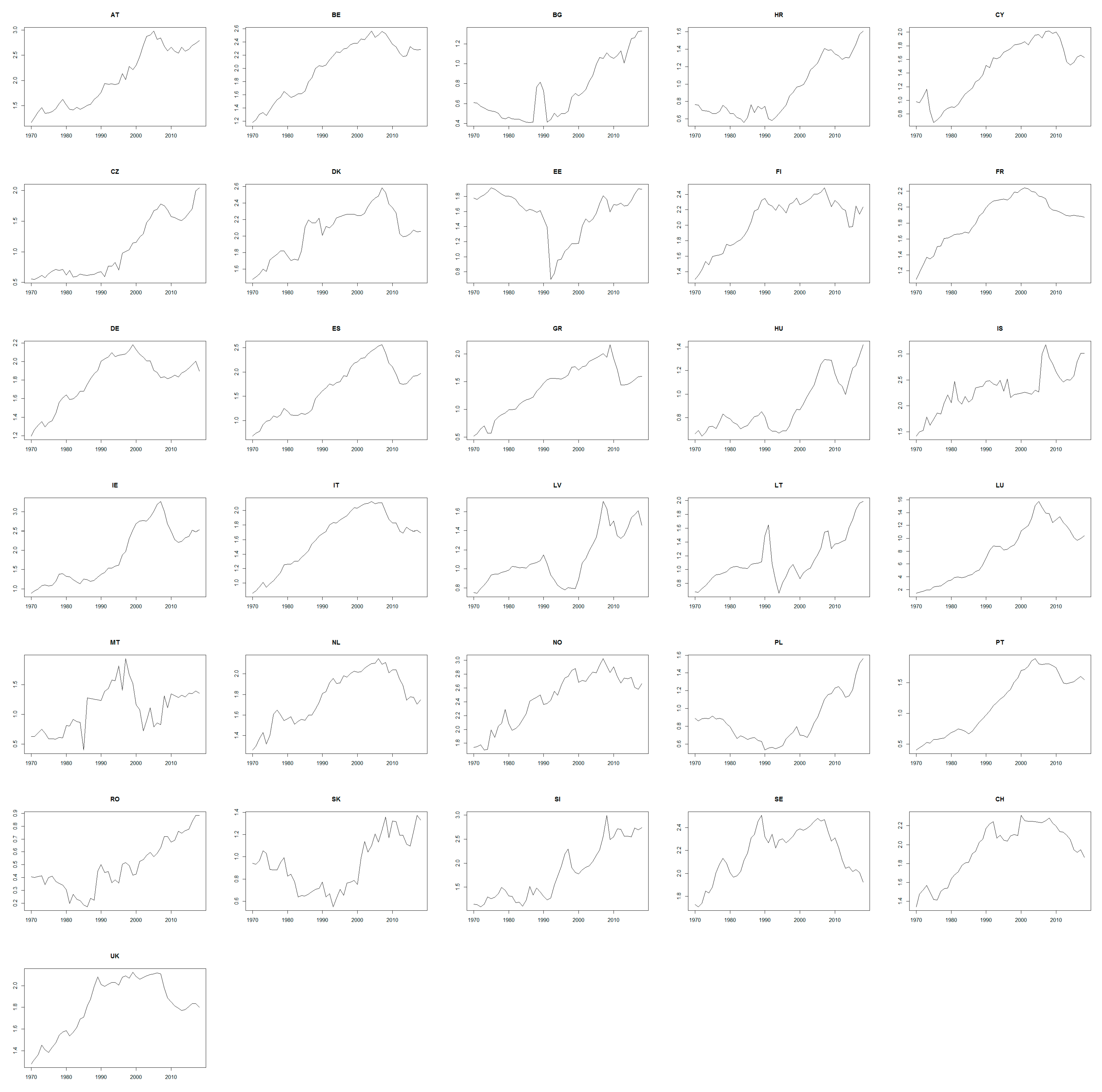
2 emissions from 1970 to 2018, filtered by the road transport sector, OECD countries, and Annex 1 adherents. In order to take into account the population of each country considered, data were transformed into per-capita emissions. The 31 countries considered were Austria, Belgium, Bulgaria, Croatia, Cyprus, Czech Republic, Denmark, Estonia, Finland, France, Germany, Greece, Hungary, Iceland, Ireland, Italy, Latvia, Lithuania, Luxemburg, Malta, the Netherlands, Norway, Poland, Portugal, Romania, Slovakia, Slovenia, Spain, Sweden, Switzerland, and the UK.
The lead–lag effect can be considered as the consequence where the change of a time-series influences another time-series with a delay [
22].
To investigate which actors can be classified as playing a leading role in the road transport emission performance, we conducted an empirical analysis of the temporal data. The investigation of the existence of a lead–lag relationship was carried out through a cross-correlation analysis in R comparing all countries with each other.
The cross-correlation between two time-series requires the time-series to be stationary.
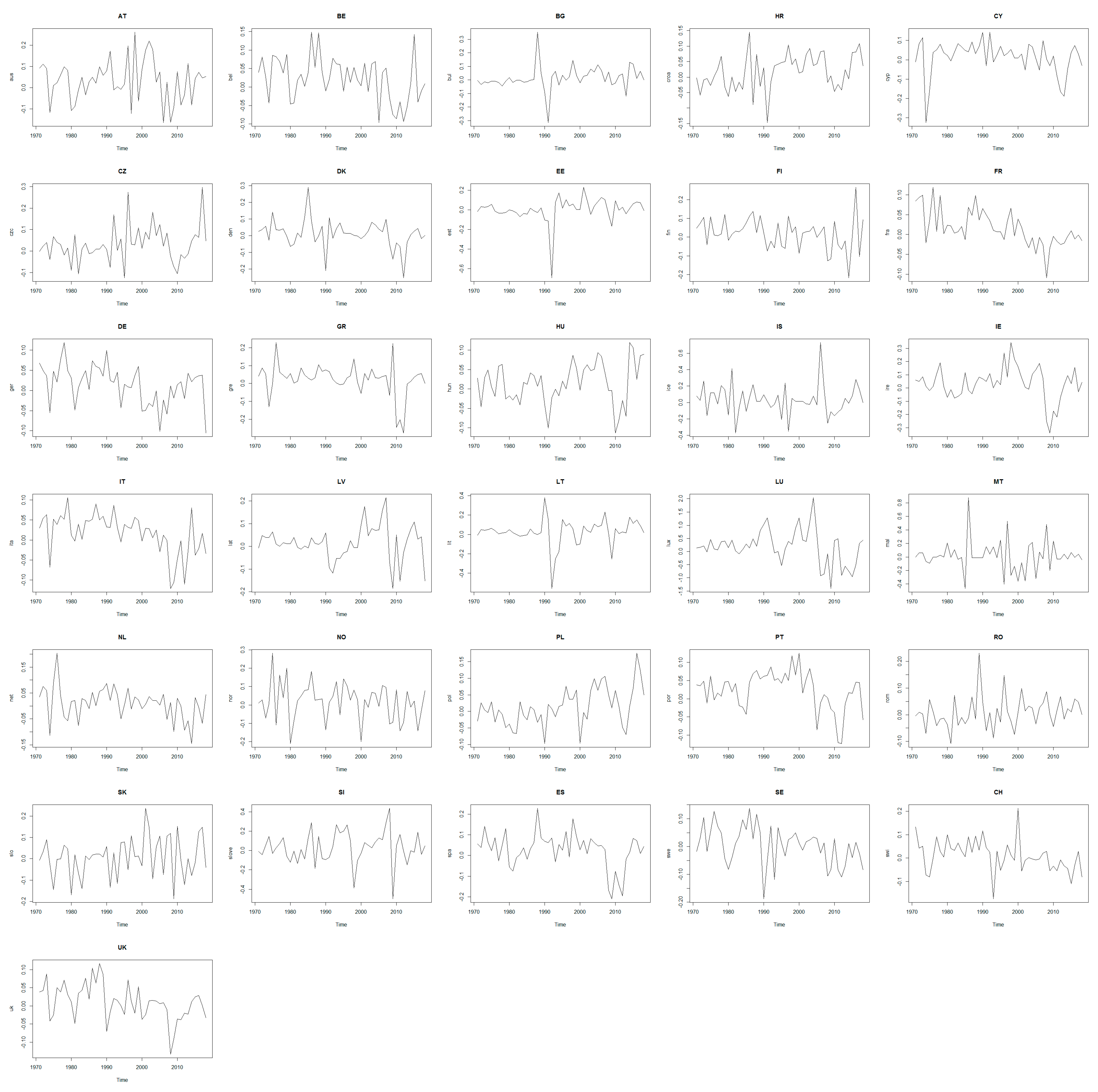
The first step in the analysis is to determine the order of integration of the road transport emission series using both the Augmented Dickey–Fuller (ADF). The ADF unit-root test is achieved on the original time-series Yt and on the time-series ∆Yt where ∆ is the first-order difference operator. For the ADF test, the null hypothesis H0 states that Yt has a unit root or equivalently the time-series is non-stationary while the alternative H1 assumes that Yt was generated by a stationary process. In particular, the ADF test assumes that the series ∆Yt follows an AR(p) process where p is usually determined comparing different formulations using the Akaike Information Criterion (AIC). The correct identification of p ensures the removal of serial correlation in the residuals of the regression. The case p = 0 corresponds to the standard (simple) Dickey–Fuller test”) test and the Kwiatkowski Phillips Schmidt Shin (KPSS). The KPSS test figures out if a time-series is around a mean or linear trend, or is non-stationary due to a unit root. In this test, the null hypothesis H0 is that Yt is stationary while the alternative H1 is that Yt contains a unit root test. All the time-series are integrated of order 1, so that the stationarity is obtained computing the first-differences. Each time-series of first-differences represents the annual emission changes.
The time-series plot of the annual emissions and annual emission changes are shown in
Figure 1 and
Figure 2, respectively.
The cross-correlation coefficients were estimated between each pair of annual emission changes.
Let us define and as two time-series denoting emissions level of countries i and j. First-differences are denoted as and .
The cross-correlation coefficient between
and
at lag
k is given by
where
denotes the Pearson correlation coefficient.
When , the cross-correlation coefficient is the relationship between the current values of and past value of . A significant coefficient implies that the former variable is affected by the latter. In this case, is the follower variable, and is the leading variable. In the present context, the annual change of emissions in country j affects the annual change in country i after k years.
When , the cross-correlation coefficient denotes the opposite relationship: the current values of are related to the future values of , that is, the current values of are related to the past values of . A significant coefficient implies that the former variable is the leading variable. In the present context, the annual change of emissions in country i affects the annual change in country j after k years
Finally, the case refers to the contemporaneous correlation between the two variables.
After estimating each cross-correlation coefficient, a hypothesis test is carried out to detect significance. The null hypothesis
is rejected, that is, the cross-correlation is significantly different from zero, if
where
is the estimated cross-correlation coefficient and
T is the length of the time-series.
In order to detect the leadership position of a country, the procedure is as follows. For each pair
, we compute the average of the significant cross-correlation coefficients with
,
, and the average of the significant cross-correlation coefficients with negative
,
. If the first average is larger, country
i is led by country
j; in the opposite case, country
i leads country
j, that is:
3. Results and Discussion
So far, we have defined the condition to identify a time-series as a leader or follower compared to another time-series [
12].
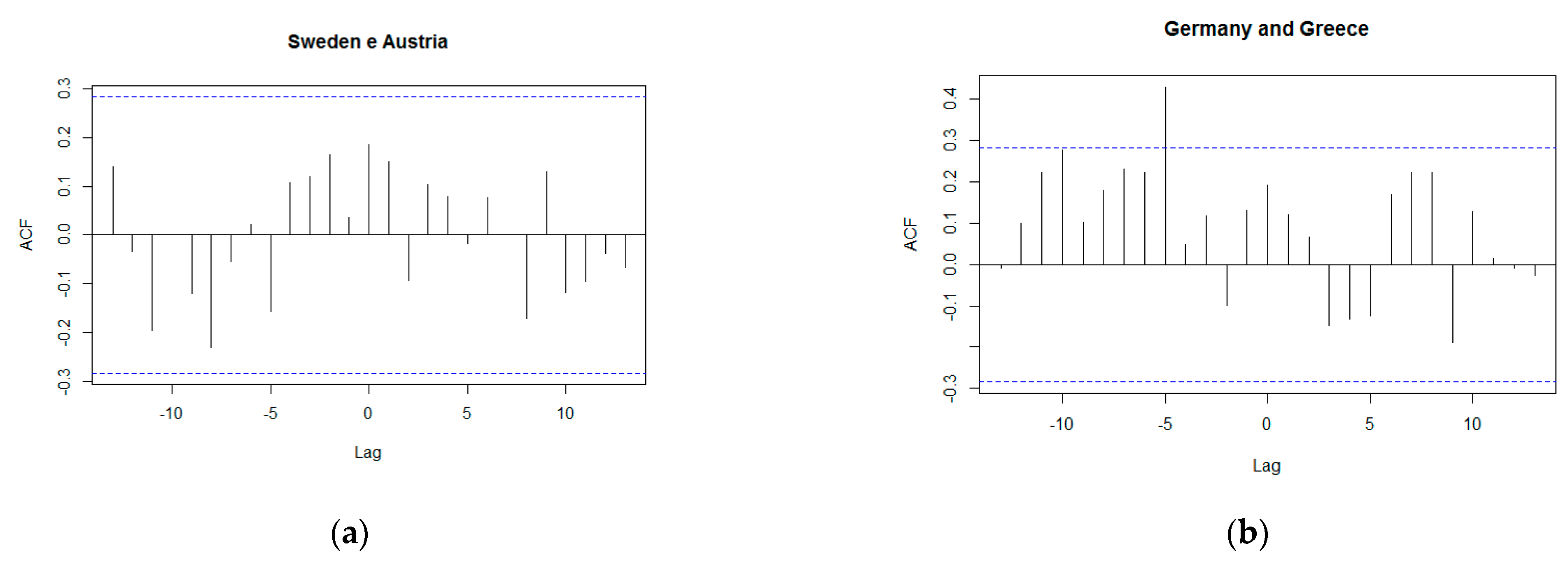
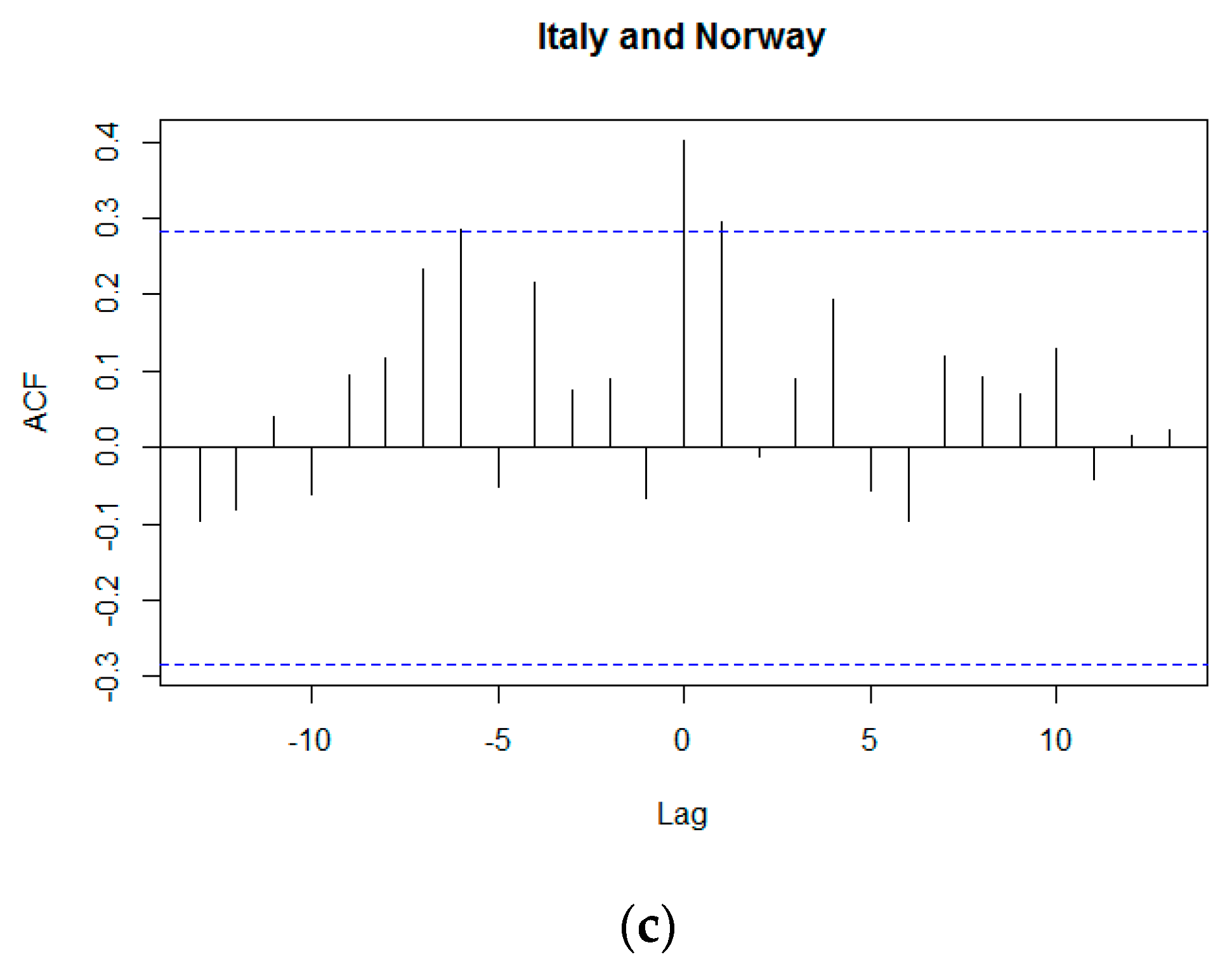
The cross-correlograms for some pairs of data are presented in
Figure 3. It shows three possible results of the cross-correlation test. In panel (a), the pair Sweden–Austria is an example of a lack of lead–lag relationship: no coefficient was significant. In panel (b), the cross-correlogram only showed one significant correlation at lag −5, which implies a leadership position of Germany on Greece. Finally, panel (c) shows that Italy was led by Norway, because the average of the significant cross-correlation coefficients with
k > 0 was larger than the corresponding average computed when
k < 0.
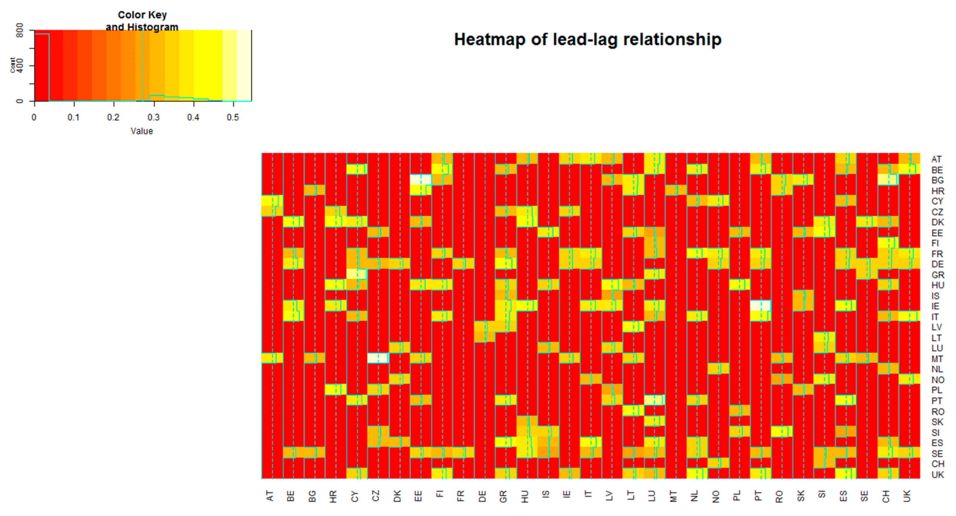
The heat map represented in
Figure 4 shows all the significant relationships coming out from the lead–lag analysis as well as their intensity. If country
i leads country
j, then the cell at the intersection of the
i-th row and the
j-th column shows
and the cell at the intersection of the
j-th row and the
i-th column will be null. So, the role as leader of a country can be analyzed by looking at the corresponding row of the heat map. For example, the role as leader played by Austria can be understood seeing the first row. We can discover that Austria has a leader role with respect to Finland, Hungary, Ireland, Italy, Latvia, Luxemburg, Portugal, Spain, and the United Kingdom. On the other hand, if country
i is led by country
j, then the cell at the intersection of the
i-th row and the
j-th column shows a null value, and the cell at the intersection of the
j-th row and the
i-th column will contain
. In this case, the role as follower of a country can be read by looking at the cells of its column. For instance, Austria (see the first column) had a follower position related to Cyprus, the Czech Republic, and Malta. Moreover, focusing on Belgium, it anticipated Cyprus, Finland, Greece, Luxemburg, the Netherlands, Portugal, Spain and the United Kingdom, but Denmark, France, Germany, Ireland, Italy, and Sweden led it. Finally, if there is no relationship between country
i and country
j, then both the cells (
i-th row,
j-th column and
j-th row,
i-th column) show null values.
In the figure, the red color denotes null values, that is, no lead–lag effect, the orange color signals a low cross-correlation, while yellow and white show a medium correlation.
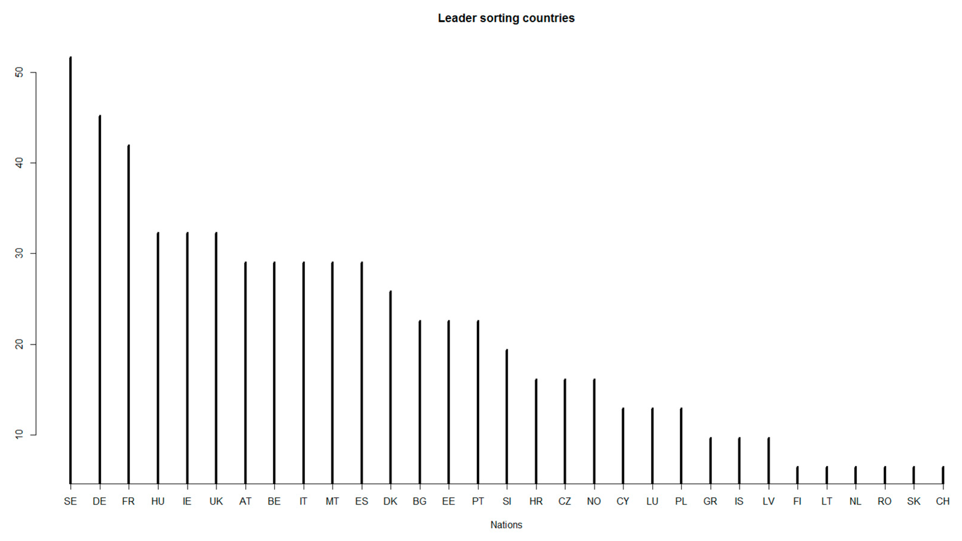
We tried to figure out which countries could be considered as the leaders in environmental road transport emissions performance. Therefore, the next step was the computation of the percentage of times a country was detected as a leader and the percentage of times a country was detected as a follower.
Figure 5 shows the rank of the 31 countries according to the percentage of times they acted as leader. A high percentage belonged to Sweden (51.6%, which means that 16 times out of 31, Sweden has resulted in being a leader country) followed by Germany (45.16%), and France (41.93%): these were the actors that most frequently resulted in playing a leading role in the field of road transport emissions reduction.
Undeniably, Sweden can be considered as a leader under numerous aspects of environmental friendly issues. Its economy is innovative oriented and its welfare system is one of the better developed between OECD countries. Sweden also has a robust environmental governance structure and a sound climate related technology. This nation has pioneered numerous policy tools, many of them based on the principle of putting a price on environmentally harmful activities. Sweden has also committed to ambitious climate goals. In fact, much progress in GHG emissions has been made. In 1991, Sweden was one of the first countries to implement environmental taxes including a tax on CO
2 reduction emissions that has been raised over time and is now among the highest in the world. In the last ten years, other environmental instruments have been introduced including a CO
2-based vehicle tax and congestion charge strategy. The last one has helped reduce city center traffic by around 20% [
23]. In Sweden, the annual circulation tax is calculated on CO
2 motor vehicle production. Furthermore, since 2011, many incentives have been in place in order to encourage the purchasing of cars with lower CO
2 emissions and the acquisition of cleaner vehicles [
24]. Moreover, the Swedish governance introduced a new bonus-malus system for the incentives and taxation of light vehicles [
25].
In this work, we also detected the strong leadership of Germany, who seems to anticipate and influence many countries. The reversal point of Germany’s time-series was around 2000, while that of other nations started around 2008. Germany was one of the first countries to implement an environmentally-friendly policy, particularly for the transport sector. The German government introduced an Eco-tax in 1999, which provided an increase in oil costs, increased cost for parking, and reduced parking space for cars.
The ecological French transition of its economy was initiated from 2007 through the adoption of the “Granelle Environment Round Table” commitments. France has a robust and extensive transport infrastructure program that has led the nation to a decrease in CO
2 emissions. By implementing the European regulation on CO
2 emissions for private vehicles and with national incentives (bonus-malus, kilometer ecotax for heavy vehicles, etc.), the reduction in vehicle production has been accelerated [
26]. From the implementation of the National Environment Plan in the 1990s, French environmental policy received new impetus thanks to the stronger incorporation of the concept of sustainable development. Concerning CO
2 emissions reduction performance, France has been made significant progress and has met its international commitments [
27].
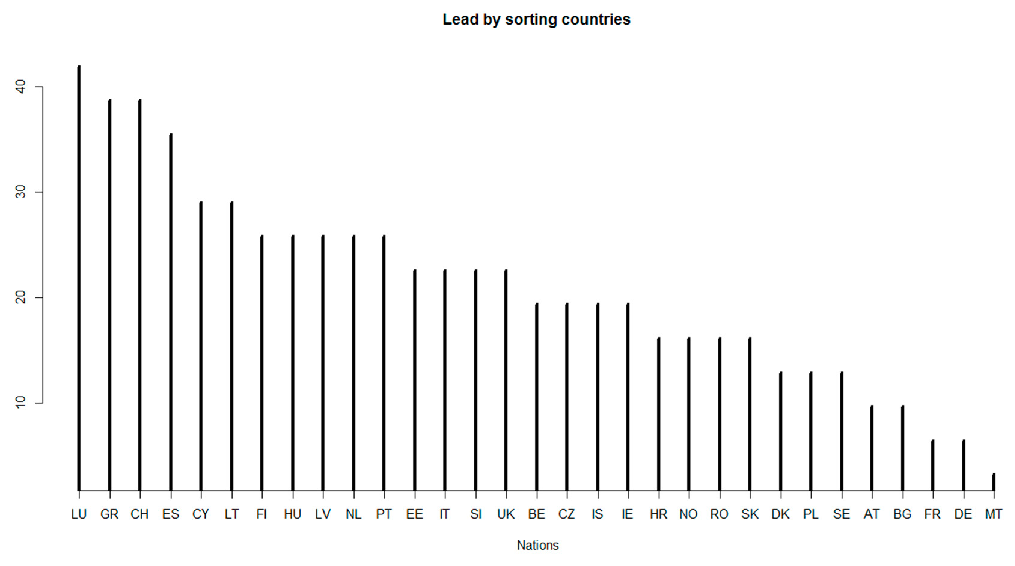
On the other hand,
Figure 6 shows the sorting of countries most frequently revealed as playing a follower role in the field of reduction in road transport emissions. The high percentages correspond to Luxembourg (41.93%), Switzerland (38.70%), and Greece (38.70%).
Nevertheless, the transport sector in Luxembourg has the biggest potential for emissions reduction; it represents more than half of the country’s GHG production. In Luxemburg, around 70% of transport emissions are caused by fuel export related to very low excise duties on fuels. In 2015, the road transport sector was one of the main sources of the total nation climate-damaging gas emissions at about 55%. Its location at the heart of the main traffic axes for Western Europe can be one explanation for this trend. Luxembourg is one of the focal points for international road traffic and therefore, traditionally has a high volume of road transit traffic for both goods (freight transport) and passengers (tourists on their way to or back from southern Europe) [
28].
The second edition of the climate action plan of Luxemburg was made public in 2013, in which 51 new measures for sustainable development were introduced. The actions were directed on different subjects from energy efficiency to the use of renewable energies, transport and environmental taxation, adaptation, and governance structures. An additional important step for the country was a change in the feed-in tariff system that came into effect only in 2014.
The Luxembourg government made reasonable green progress when all public transportation became free to users, the tram network was expanded, and support for the purchase of e-bikes was provided.
The country has made progress toward emissions reduction development goals though its current target of a 40% reduction compared to 2005, to be achieved by 2030, appears quite ambitious.
Part of this new strategy is the decline in fuel consumption, and future emissions reduction goals are to be attained through a CO
2 tax, electrification of automobile traffic, introduction of higher energy-efficiency, and replacement of oil heating with renewable energy sources [
29].
Switzerland accounts for about one third of end energy consumption with an upward tendency. The largest contributor of Swiss CO
2 emissions has been road traffic. It has been levying a CO
2 tax since 2008, nevertheless, the major emissions sector is road transport, where private passenger vehicles account for two thirds of them. Switzerland, like Luxemburg, has an important geographical position for transport, import, and export trips. Furthermore, the inadequate impact of transportation to Swiss CO
2 emissions reduction is also due to a context of moderately strong demographic and economic growth between 1990 and 2015 [
30].
In Greece, the transport sector remains a major source of air GHG emissions as improvements in vehicle and fuel quality have been outweighed by increasing transport volume. Particularly, road transport is the main cause of all climate-damaging gas emissions, with the exclusion of SOx, which is mostly due to navigation. The Greek emissions growth by road and navigation transport has risen by 22%. Furthermore, due to the renewal of the road vehicle fleet, emissions fell by over 30% between 2000 and 2006 [
31].
4. Conclusions
In this article, the detection of lead–lag relationships on the road transport emission time-series was made through the application of the cross-correlation function. The world community has repeatedly recognized the importance of leadership in the field of climate change and past agreements have explicitly identified which country is supposed to shoulder the mantle of leadership. Previous research on leadership for climate change aspects has been conducted mainly by surveys based on the perception of leaders among the United Nations Framework Convention on Climate Change participants.
This paper contributes to the existing literature by providing new evidence on the empirical lead–lag analysis in environmental studies. By analyzing 31 OECD nations and Annex 1 adherents, our studies specifically focused on the identification of which country played a predominately role of leader in the reduction of road transport emissions performance. The time-series examined in this project were extracted from the EDGAR database, which contains estimates of fossil CO2 emissions from 1970 to 2018.
Emissions provoked by road transport are expected to grow at a faster rate than other sectors, posing a major challenge to efforts in order to reduce CO2 production in line with the Paris Agreement and other global goals. Many OECD countries have tried to give their contribution by following and undertaking measures in order to reduce CO2 phenomena due to road transport by focusing on different aspects for example, like voluntary agreement between vehicle manufacturers and government, the production of low-fuel consumption vehicles, the introduction of graduated vehicle taxes, fuel taxes, and excise duties. OECD authorities are increasing and promoting strategies to expand the use of more environmentally-friendly vehicles, which turns into the improvement of the efficiency of public transport.
In order to confirm our outcomes, we rewired the environmental policy history of the countries and found some explanations regarding the emissions trend. The results of the lead–lag analysis showed that countries such as Sweden, Germany, and France have led many others. Therefore, the nations that are classified as the top-leader countries have introduced earlier regulations in their national laws to support the environmentally-friendly mechanisms. On the other hand, Luxemburg, Switzerland, and Greece are considered as “follower” countries. This could be persuasive intuition due to their strategic geographical positions, which defines them as transit nations because of their properties as focal points for shipping and travel connections.
The rapid growth of CO
2 emissions and its possible solutions continue to attract researcher interest under different aspects. The authors in [
32] showed the importance of transport energy efficiency related to the negative environmental impact of this sector. They believed that energy efficiency in transportation should be measured by CO
2 emissions. The study in [
3] considered the seven largest carbon-emitting economies and studied their CO
2 emissions trend in the transportation sector. They claim that a planned energy structure and limited private car ownership play an important role in CO
2 decrease.
The most effective approach of reducing GHG emissions from proper cars and road transport should involve a package or combination of measures that promote the effectiveness of the local policy makers and at the same time takes measures by thinking of their potential position at the local level.
Moreover, many academics have highlighted the importance of developing effective local policy planning for environmentally-friendly performance. However, data for road transport emissions are predominantly prepared at the national level, for example, reference [
33] focused their study on a new approach to scale down national level emissions to smaller areas. This process could be externally useful to policy-makers in order to identify the major emissions problems to be addressed.
The transition from old to alternative fuel mechanisms continue to decelerate and only helps to slow their impact on CO2 emissions. Indeed, vehicles powered by environmentally-friendly energies are costly, and only few countries have the power of an extensive restocking network; this leads, as a result, to a slow process, which creates a difficulty for the entrance of this type of vehicle on the market. CO2 reductions can only be achieved by taking measures at both the national and international levels, where many other variables play a significant role for a positive environmental performance such as the population’s awareness to environmental issues, the culture, the education, the different typology of government, consumer information, and the promotion of greater fuel efficiency in the different sectors involved.
Furthermore, another important aspect considered by researchers is the innovation of technologies and economies. Indeed, reference [
34] studied the relationship between the absorptive capacity on innovation and CO
2 in China and the USA, finding that an increase in absorptive capacity and infrastructure development provided benefits in order to mitigate the carbon intensity. Additionally, reference [
35] studied the role of Dutch institutions in public transport and believe that institutional innovation helps the transition to zero emissions public transport in the Netherlands. They also showed many barriers that actually discourage this transition to the use of battery electric and hydrogen fuel for public transport.
In this research, we have tried to provide an explanation lingering on the introduction of environmental regulation, but it would be interesting to verify the existence of other variables that could influence the emissions trend and so determine the relationship between the leader or follower classification countries.


