The Influence of Seasonal Meteorology on Vehicle Exhaust PM2.5 in the State of California: A Hybrid Approach Based on Artificial Neural Network and Spatial Analysis

Abstract

This study aims to develop a hybrid approach based on backpropagation artificial neural network (ANN) and spatial analysis techniques to predict particulate matter of size 2.5 µm (PM2.5) from vehicle exhaust emissions in the State of California using aerosol optical depth (AOD) and several meteorological indicators (relative humidity, temperature, precipitation, and wind speed). The PM2.5 data were generated using the Motor Vehicle Emission Simulator (MOVES). The measured meteorological variables and AOD were obtained from the California Irrigation Management Information System (CIMIS) and NASA’s Moderate Resolution Spectroradiometer (MODIS), respectively. The data were resampled to a seasonal format and downscaled over grids of 10 by 10 to 150 by 150. Coefficient of determination (${\mathrm{R}}^2$), mean absolute percentage error (MAPE), and root mean square error (RMSE) were used to assess the quality of the ANN prediction model. The model peaked at winter seasons with ${\mathrm{R}}^2$ = 0.984, RMSE = 0.027, and MAPE = 25.311, whereas it had the lowest performance in summer with ${\mathrm{R}}^2$ = 0.920, RMSE = 0.057, and MAPE = 65.214. These results indicate that the ANN model can reasonably predict the PM2.5 mass and can be used to forecast future trends.

1. Introduction

Nowadays, there is a unanimous scientific consensus that air quality degradation leads to adverse health effects [1]. One of the factors impacting the air quality index is suspended particulate matter, which is associated with numerous human diseases. Health problems from particulate matter can generally be classified as those caused by coarser particles targeting the lower respiratory system and those caused by finer particles targeting the lung’s gas-exchange region. The coarser particles are classified as those with diameters smaller than 10 $\mathsf{\mu }$m (PM10), whereas the finer particles correspond to those with diameters smaller than 2.5 $\mathsf{\mu }\mathrm{m}$ (PM2.5). Both classes of particulate matter are highly dependent on climatic factors such as precipitation, relative humidity, wind speed, and air temperature, and are positively correlated with the aerosol optical depth (AOD) [2,3]. In particular, AOD, which can be retrieved from remote sensing products, is considered a good proxy for PM2.5 [4].

Anthropogenic activities and natural emissions are the primary sources of PM2.5 in the western United States. Natural emissions of PM2.5 consist of wind-blown dust [5,6], biogenic non-methane volatile organic compounds (NMVOCs) [7], sea salt, wildfires, and lightning NOx emissions [8]. The sharp pulses in PM2.5 mass time-series during the summer season resulting from wildfires are also significant contributors to air pollution in this region [9]. Examples of anthropogenic activities are agricultural burning, construction and demolition activities, industrial processes, and mobile emissions. In general, the spatial distribution of anthropogenic PM2.5 emissions is highly dependent on population density. Currently, motor vehicles substantially contribute to air pollution, accounting for 65% of total PM2.5 emissions in urban areas in the United States [10]. Mobile emissions contain the fuel combustion exhaust from different vehicle types, which can be determined using the Motor Vehicle Emission Simulator (MOVES) [11]. MOVES is an emission modeling system that estimates emissions from on-road motor vehicles and most off-road equipment nationwide.

There are several statistical techniques for particulate matter distribution forecasting, among which, the artificial neural network (ANN) is expected to have a better performance compared to classical linear and non-linear regression methods [1]. The reason for better performance is that ANN has a better adaptation capability in highly non-linear physical processes [1]. Moreover, a hybrid method based on ANN and spatial analysis is expected to produce a more reliable model for particulate matter prediction. Hence, the study aims to develop a working model of particulate matter dispersion based on AOD using meteorological variables as auxiliary inputs. Three relatively recent years (2010, 2014, and 2018) were selected to calibrate, validate, and test the model, and the U.S. state of California was chosen as a case study due to high levels of particulate matter in this region. Although the model was developed for California, it can be applied to other regions worldwide, given the widespread availability of the input data used in this research.

The remainder of the paper is organized as follows: First, a literature review is presented to summarize the results of similar studies regarding the prediction of PM2.5 with a particular focus on ANN models. The materials and methods section primarily focuses on the spatial analysis of data and ANN’s mathematical theory. Specifically, this section explains model input and target variables, including MOVES generated PM2.5, AOD from NASA’s Moderate Resolution Spectroradiometer (MODIS), and meteorological data from California Irrigation Management Information System (CIMIS). The major contribution of this study is an ANN model for PM2.5, which is calibrated and assessed in the results and discussion section. Lastly, recommendations are provided to further highlight the practical aspect of the model.

2. Literature Review

In this section, a condensed and focused literature review is presented. For an in-depth review, the reader is referred to [12].

2.1. Classical Regression Models for Particulate Matter

Motor vehicles contribute 10% to 65% of total PM2.5 emissions in urban areas in the United States [10]. To assess the impacts of transportation projects on air quality and to identify the projects classified as a Project of Air Quality Concern (POAQC), Reid et al. (2017) used both the MOVES and the emission factors model (EMFAC) based on quantifying PM10 and PM2.5 emissions in an analysis conducted for the year 2006. Their goal was to evaluate the impact of fleet turn-over and truck use percentages on future project-level emissions [13]. Comparing the two models, they concluded that tire wear and re-entrained road dust emissions from both models were roughly equal. However, MOVES exhaust emissions estimates for 2006 were about 70% higher than the EMFAC estimates. On the other hand, EMFAC brake wear estimates were 2.5 times higher than the MOVES estimates [13].

Multiple regression approaches are used to define the correlation between particulate matter, AOD, and meteorological products. Gupta and Christopher (2009) developed a simple two-variate method (TVM), where AOD observed by MODIS was initially used to estimate surface-level PM2.5 concentration. Later, they gradually added meteorological parameters to the built model to form a multiple variate method (MVM). In their study, PM2.5 mass was obtained from the Environmental Protection Agency (EPA), and satellite aerosol data were obtained from the MODIS [14]. The study used a rapid update cycle (RUC) to extract meteorology data, including air temperature at 2 m, surface relative humidity, wind speed at 10 m, and height of the planetary boundary layer [14]. The results showed that applying the MVM model improved the accuracy of the TVM model’s hourly and daily average PM2.5 values by 13% and 17%, respectively [14].

2.2. ANN Models for Particulate Matter

A neural network can learn particular skills by utilizing three layers: the input layer, hidden layer, and output layer [14]. The input layer receives input data, which in most cases, are physical characteristics of a complex phenomenon. The output layer receives the desired output data and typically is limited to a single variable. There is a hidden layer between the input and output layers that establishes a non-linear relationship between the input and the output data. This operation is accomplished by nodes (neurons) embedded in the hidden layer simulating the actual human brain function. These nodes receive the input, multiply it by weight, add a bias, and then pass it to the output. This procedure is repeated until the hidden layer output converges to the initial output (called target data). The governing equations will be discussed in depth in the Materials and Methods section.

The complexity inherited in particulate matter distribution makes the ANN an ideal candidate. In the study conducted by Gupta and Christopher (2009), the ANN model improved particulate matter estimation accuracy by 23%. Compared with the TVM and MVM models, ANN was found to have a greater capacity to reduce the absolute percentage error [14]. A similar study was conducted by Zaman et al. (2017), who used multiple linear regression (MLR) and an ANN to conduct regression analyses on particulate matter, meteorology variables, and AOD. The meteorological data and AOD values were obtained from satellites. The ground-based measurements were only used for validation due to their low spatial resolution. The coefficient of determination (${\mathrm{R}}^2$) of the ANN approach was 0.71, and the root mean square error (RMSE) was 11.61 μg m⁻³, which was better than the MLR results (${\mathrm{R}}^2$ = 0.66 and RMSE = 12.39 μg m⁻³) [15]. Thus, the ANN model was designated as being superior over the linear regression model.

To deal with low spatial resolution problems encountered in [15], Enotoriuwa et al. (2018) used spatial interpolation. In their study, a 10 by 10 grid was generated over the study location [16]. The interpolated data were then downscaled to the grid points to improve the spatial resolution. After removing the grids with outliers, the total number of the remaining nodes for regression was 108 [16]. This approach resulted in ${\mathrm{R}}^2$ values of 0.65 and 0.58 for PM2.5 and PM10, accordingly.

There are also particulate matter related studies frequently conducted in the Beijing–Tianjin–Hebei (BTH) area since the particulate matter is a significant contributor to haze weather and air quality in this region. For example, Wu et al. (2012) used a backpropagation ANN algorithm to estimate particulate matter in the BTH area using AOD and other meteorological data. In this study, the number of nodes in the hidden layer varied from six to 15 [17]. In terms of the correlation between observed and estimated particulate matter concentrations, most models’ correlation coefficient values were greater than 0.4 [17]. Another study conducted by Yi et al. (2019) in the same area used three models: backpropagation ANN, support vector regression (ε-SVR), and combined backpropagation ANN and ε-SVR. These models were used to estimate the missing historical values of PM2.5 [18]. ANN and ε-SVR had similar performance in terms of the correlation coefficient values. However, combining the two methods further improved the accuracy of their estimates. This method was suitable for the BTH area but could be extended to other locations as well [18].

The present study was developed based on the assumption that the particulate matter is positively correlated to the AOD levels. Additionally, it builds upon the studies mentioned above to develop a working model of particulate matter for California. In particular, monthly PM2.5 data were generated [13], monthly observed meteorological data were acquired [14,19], spatial analysis was utilized to improve low-resolution data [16], and eventually, the ANN approach was used to develop an accurate model for particulate matter spatial distribution [15,17,18]. The novelty of this investigation is an in-depth study of the spatial resolution and the seasonal meteorological impact on the use of model-generated particulate matter.

3. Study Area

The study area for this research was the state of California (Figure 1), which is located on the west coast of North America (Latitude: 36.7783° N, Longitude 119.4179° W). California faces the Pacific Ocean on the west and is bounded by Oregon on the north, by Arizona and Nevada on the east, and by the Mexican state of Baja California on the south. Northern and central California have a Mediterranean climate, whereas the southeast of California is classified as arid [20]. California’s average temperature is around 25 °C, and the average annual precipitation is approximately 457.2 mm. California is the most populous state with the largest economy in the United States. It consists of 58 counties and has two large megalopolises: one in southern California and one in the Bay Area. The number of registered automobiles in California was 14.6 million in 2017, making it a significant contributor to particulate emissions.

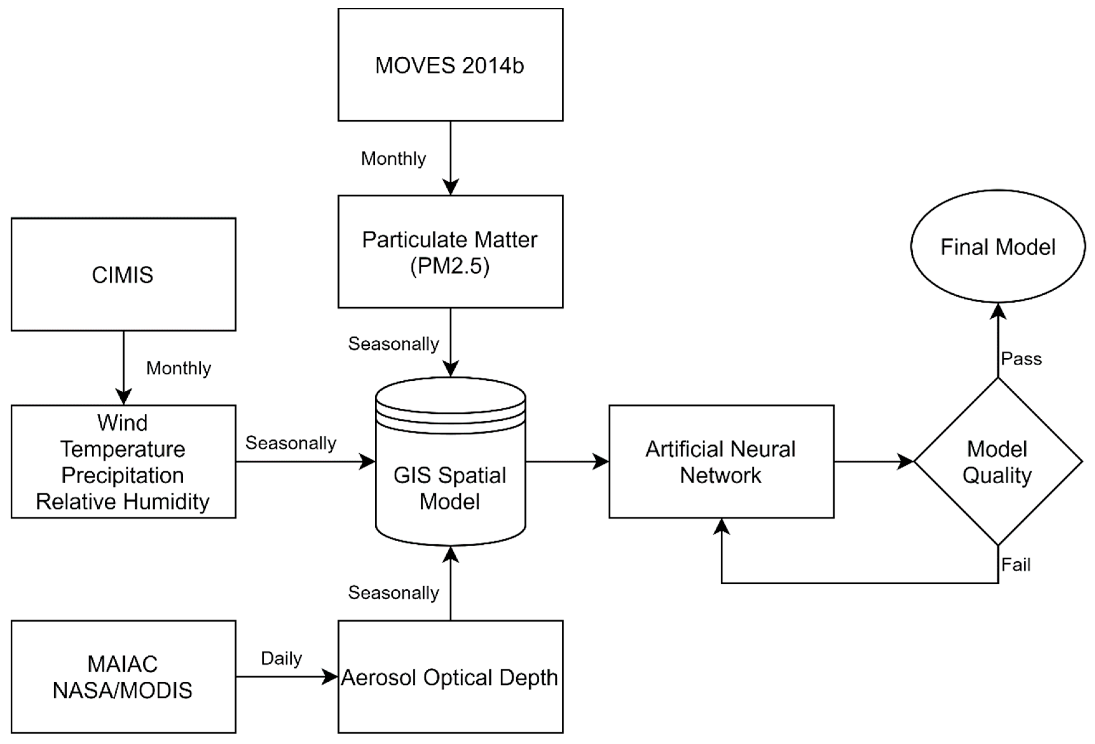
4. Materials and Methods

This study benefits from modeled PM2.5, measuring stations (temperature, wind speed, precipitation, and relative humidity), and observational satellite data (AOD). The measured and satellite data are available at different spatial and temporal resolutions; for example, PM2.5 and meteorological variables are available monthly while AODs are available daily. A seasonal time scale was chosen for this study, so data were scaled up to create seasonal averages. The Northern meteorological seasons are spring (March, April, and May), summer (June, July, and August), fall (September, October, and November), and winter (December, January, and February). The procedure for data processing is shown in Figure 2, in which the input data are fed into the spatial model for rescaling purposes.

Three recent years of 2010, 2014, and 2018 were selected as a case study to analyze the annual trends. As for the spatial measure, the data were resampled over uniform grids generated in Figure 3. These grids were initially created as squares with tiles of 10 by 10 (100 km by 100 km), 20 by 20, etc., through 150 by 150 (7 km by 7 km) and were overlaid on the state of California. Then, only the grids falling inside the California boundary were kept. The grids with tiles larger than 80 by 80 were not recognizable and therefore were not included in Figure 3. Once the temporal and spatial resolutions of data were adjusted, an ANN model was developed based on the meteorological and AOD values as input and PM2.5 mass as the target. This is also shown in Figure 2, where the processed data are fed from the spatial model to the ANN model.

4.1. Artificial Neural Network (ANN)

ANNs are systems that imitate the mechanics of neural association in the human brain rather than implementing specific governing equations. The neural network has a robust non-linear mapping ability, which generates a more flexible functional relationship between the input and target data [21]. A feed-forward neural network was established to determine the non-linear relationship between input data and PM2.5. This ANN model consisted of an input layer, an output layer, and a hidden layer. Increasing the number of hidden layers can create a deep neural network known as deep learning. The architecture of the feed-forward ANN, together with input and output parameters, are depicted in Figure 4. As shown in Figure 4, five input parameters, including precipitation, air temperature, relative humidity, wind speed, and AOD, were fed in the input layer to estimate the PM2.5 mass in the output layer.

Each layer may have multiple nodes/neurons that simulate the biological system by receiving signals from other neurons and transmitting to the next neurons. Each neuron is the output of the previous layer and input for the next layer. The arrow connections in Figure 4 represent the weights in ANN through which neurons interact [22]. The neurons in the hidden and output layer are calculated through the weight connection and net input function. The net input can be expressed as

$$n={\displaystyle \sum }_{j=1}^R{w}_j{p}_j+b=Wp+b$$

(1)

where $p_j$ represents the input parameter, defined as the elements in the input vector $P=\left[p_1,p_2,\dots ,p_R\right]$ with corresponding weights of $W=\left[w_1,w_2,\dots , wj\right]$. The input $p_j$ is multiplied by the weight and added to bias ($b$) to form the net input. Bias is an intercept to adjust the weighted sum of the net inputs to the neuron. The transfer function to process the net input to obtain the neuron output is calculated by

$$a=f\left(n\right)$$

(2)

with $f$ as the activation function. In this study, the log-sigmoid activation function was adopted as

$$f\left(x\right)=\frac{1}{1+e^{-x}}$$

(3)

During the network training, the input parameters, number of neurons, and layers are preset. The network characteristics are stored in the form of weights and biases. This information, together with Equations (1)–(3), makes the output a function of weights and biases. In this study, the training was accomplished using Levenberg–Marquardt backpropagation, a hybrid algorithm combining backpropagation and Newton’s method. The process of backpropagation involves adjusting the weights and biases in the network to minimize the error between the target and output values. This concept can be turned into a cost function ($\widehat{F}$) expressed as the mean square error ($e$) for the $q$th input/output pair by

$$\widehat{F}=\frac{1}{2}{e}_{-q}^T{e}_{-q}$$

(4)

The process of cost function minimization was performed using gradient descent. The gradient is the derivative of the cost function calculated with respect to the weights and biases and expressed as $\frac{\partial \widehat{F}}{\partial W}$ and $\frac{\partial \widehat{F}}{\partial b}$, respectively. The process is finding a slope that leads the steepest descent to reach the local minimum of the function, i.e., the error between target and output is minimized. In the Levenberg–Marquardt algorithm, the Jacobian matrix was introduced during the computation of gradient descent. The Jacobian matrix requires calculating the derivatives of the network’s errors instead of the mean square errors [23]. This can be computed as

$$g=J^{T}e$$

(5)

where $e$ is the vector of network errors, and $J$ is the Jacobean matrix that contains first derivatives of the network’s errors with respect to biases and weights [24]. The second derivative of the network’s errors can be expressed as a Hessian matrix by

$$H=J^{T}J$$

(6)

Applying the Gauss–Newton method, the Levenberg–Marquardt algorithm can be written as

$$x_{k+1}=x_k-{\left[H+\mu I\right]}^{-1}{J}^{T}e$$

(7)

The parameter $x_k$ represents weights and biases at iteration step $k$ with $I$ as an identity matrix, and $\mu$ as a damping factor. When $\mu$ increases, the function becomes closer to the gradient descent, slowly reaching the minimum error. As $\mu$ decreases (getting closer to zero), the algorithm reverts into Newton’s method. Newton’s method is faster and more accurate near the error minima [24].

4.2. Particulate Matter

Contrary to the previous studies that utilize in-situ particulate matter measurements, this project benefits from the modeled particulate matter estimates. While acknowledging the availability of the directly measured data [25,26], it was not feasible to incorporate them into this study. Since the study’s focus was PM2.5 from vehicle emissions, and to date, there has not been any direct measurement available for car emissions. The only available data were from Don Stedman’s group at the University of Denver [27,28] but the temporal and spatial resolutions of this data were not sufficient to serve the purpose of this study.

Therefore, particulate matter values were generated using the United States Environmental Protection Agency’s Motor Vehicle Emissions Simulator (EPA MOVES). The MOVES model contains relevant vehicle emission inventory for the entire United States. The MOVES framework includes four different parts: the total activity generator (TAG), the source bin distribution generator (SBDG), the Operating Mode Distribution Generator (OMDG), and the emission calculator [11]. TAG uses base year vehicle population and vehicle miles traveled (VMT) to analyze yearly growth factors and categorizes them by road type, vehicle type, vehicle age, and time [29]. MOVES uses discrete binning when evaluating emissions, in which each type of traffic activity is binned into a single data point based on the fuel consumption of automobiles [29]. In the process of differentiating exhaust emissions, the vehicle specific speed (VSP) was defined for light-duty vehicles and the scaled tractive power (STP) for heavy-duty vehicles [30]. The VSP and STP values depend on the vehicle mass, dynamic parameters, speed, acceleration, and gravitational acceleration. The mathematical form of modeling equation for light-duty and heavy-duty vehicles was [31]

$$VSP \mathrm{or} STP=\left(\frac{A}{M}\right)v+\left(\frac{B}{M}\right)v^2+\left(\frac{C}{M}\right)v^3+\left(\frac{m}{M}\right)\left(a+g\ast \sin \theta \right)v$$

(8)

where $A$ is the coefficient of rolling resistance (kW-s m⁻¹), $B$ is the coefficient of rotational resistance (kW-s² m⁻²), $C$ is the coefficient of aerodynamic drag (kW-s³ m⁻³), $v$ is the instantaneous vehicle speed (m s⁻¹), $a$ is the instantaneous acceleration (m s⁻²), $M$ is the fixed mass factor for the source type (metric tons), $m$ is the vehicle mass (metric tons), $\theta$ is the road grade (fractional), and $g$ is the gravitational acceleration (9.8 m s⁻²). The m/M ratio of light-duty vehicles was assumed to be 1.0. The M in the heavy-duty vehicles formula was approximately the average running weight for all heavy-duty vehicles [30].

In creating the emission output using the MOVES 2014b model [11], the emission analysis scale was set to nationwide on-road vehicles. The defined time scale for calculation was monthly, and the geographic boundary was set to the state of California. The output of the model was the mass of particulate matter in kilograms per county. The mobile sources of emissions consisted of on-road vehicles of all fuel types. The particulate matter emission was generated for all road types with the 1990 Clean Air Act Amendments implemented, and the output data and the reported units were stored in the output database.

4.3. Aerosol Optical Depth (AOD)

Aerosol consists of fine solid particles and liquid droplets in the atmosphere. It can absorb and scatter rays of light that pass through it. Often, the wavelength at 0.55 $\mathsf{\mu }$m is used for aerosol retrieval from the satellite images. AOD, a dimensionless positive value, is a measure of extinction of the solar irradiance at a specific wavelength. It represents the aerosols distributed within a column of air from the Earth’s surface to the top of the atmosphere. The AOD magnitude range is from 0 to 1, where 0 represents an entirely transparent atmosphere, and 1 represents an entirely opaque atmosphere. The relationship between AOD and solar irradiance at a specific wavelength of λ can be described by the Beer–Lambert law by

$$I\left(\lambda \right)=I_0\left(\lambda \right)\exp \left[-{\tau }_a\times m\right]$$

(9)

where $I_0\left(\lambda \right)$ is solar irradiance of extra-terrestrial, which is considered as solar constant, $I\left(\lambda \right)$ is solar irradiance at a wavelength of $\lambda$ at the Earth’s surface, ${\tau }_a$ is the atmospheric optical depth, and $m$ is the optical air mass, which can be calculated as relative air column length of zenith angle θ at that of zenith direction 1. The solar radiation diminishes due to scattering and absorption by atmospheric elements such as air molecules, aerosols, water vapor, carbon dioxide, and ozone. Therefore, to calculate the aerosol optical depth, it is required to eliminate the optical depth of air molecules, water vapor, and other atmospheric elements.

AOD values reflect the real-time particulate matter concentration in the atmosphere. The AOD data used in the analysis were extracted from the databases on the MODIS website. The MODIS is an essential remote sensor onboard NASA’s satellites, Terra and Aqua. Both satellites scan the entire surface of the earth for various data [32]. Typically, MODIS is used for acquiring information on aerosols, ocean color, cloud, and ozone. In this study, the daily AOD product used is from MCD19A2 version 6 of MODIS (https://lpdaac.usgs.gov/products/mcd19a2v006/). These data are generated by an algorithm for multi-angle implementation of atmospheric correction (MAIAC) [33]. Combining Terra and Aqua values can improve cloud detection accuracy, aerosol retrieval, and atmospheric correction.

The downloaded MCD19A2 hierarchical data format (HDF) files include daily AOD gridded level 2 data at 1 km (km) pixel resolution [33]. MODIS terrestrial data are distributed in non-overlapping tiles in sinusoidal projection. The shape of the tiles is approximately square and measure 10 degrees by 10 degrees at the equator. The tile coordinate system starts at the upper left corner of the map and proceeds right (horizontally) and down (vertically). The horizontal axis is divided into 36 segments (0–35), and the vertical axis is divided into 18 segments (0–17) [34].

4.4. Meteorology

The daily meteorological data used in the study were collected from the CIMIS. The CIMIS department operates 259 weather stations, including 157 active (had data for the study period) and 102 inactive stations (did not have data for the study period). The locations of weather monitoring stations are depicted in Figure 1 as triangles. The sensors can collect weather data on a minute by minute basis. The hourly and daily data are calculated and stored in the data loggers and automatically transferred to the central computer for further analysis and correction. The processed data are stored in the central database server and are available on the CIMIS website [35].

The meteorological data used in this study for modeling were precipitation (P), relative humidity (RH), wind speed (W), and air temperature (T). The sensor for air temperature and relative humidity was a Fenwal Thermistor/HUMICAP H-sensor. The range of detection was −35 to +50 °C for the temperature and 0 to 100% for the relative humidity. The wind speed sensor is a three-cup anemometer utilizing a magnet-activated reed switch. The frequency of this anemometer is proportional to wind speed. The instrument’s height is 2.0 m and can measure the wind speed of 0 to 100 mph. A tipping bucket rain gauge with a magnetic reed switch is used to record the precipitation, and the accuracy of the sensor is within 1%.

5. Results and Discussion

5.1. Seasonal Pattern of PM2.5

Figure S1 shows the MOVES estimated PM2.5 seasonal distribution in California counties in units of kg. The color bar range and style were kept consistent for all the choropleth maps. According to Figure S1, the spatial variation of PM2.5 was generally more significant than its temporal variations. The highest PM2.5 mass was observed near southern California, while the lowest values occurred in the north and eastern California regions. This is attributed to the fact that Los Angeles County has the highest and Alpine County has the lowest number of registered vehicles in the state, based on California’s Department of Motor Vehicle report for the year 2019 [36]. Seasonally, summer received the highest maximum PM2.5, whereas winter received the lowest maximum PM2.5 (

Table 1. County-level maximum and minimum seasonal PM2.5 in the state of California for years 2010, 2014, and 2018.

	Maximum PM2.5 (kg)			Minimum PM2.5 (kg)
Season/Year	2010	2014	2018	2010	2014	2018
Summer	3.0 × 105	2.0 × 105	1.6 × 105	2.9 × 102	1.9 × 102	1.6 × 102
Spring	2.9 × 105	1.9 × 105	1.5 × 105	3.0 × 102	2.0 × 102	1.6 × 102
Fall	2.8 × 105	1.9 × 105	1.5 × 105	3.0 × 102	1.9 × 102	1.5 × 102
Winter	2.7 × 105	1.8 × 105	1.4 × 105	3.2 × 102	2.1 × 102	1.6 × 102

). On the other hand, winter received the highest minimum PM2.5, whereas summer received the lowest minimum PM2.5 (Table 1). This is attributed to the driving habits, motives, and attitudes of state residents [37].

5.2. Seasonal Pattern of AOD

In this study, the AOD files were obtained when the satellites traversed the study domain, with filenames h08v04.hdf, h08v05.hdf, and h09v04.hdf. They represent the three tiles covering the state of California.

Table 2. Mosaic aerosol optical depth (AOD) files in hierarchical data format (HDF) covering the state of California.

File Name	Min Longitude	Max Longitude	Min Latitude	Max Latitude
h08v04	−155.5724	−117.4758	40.0000	50.0000
h08v05	−130.5407	−103.9134	30.0000	40.0000
h09v04	−140.0151	−104.4217	40.0000	50.0000

shows the minimum and maximum latitude and longitude of these tiles. In the filenames, “h” stands for horizontal, and “v” stands for vertical. Post-processing was performed to generate seasonal data using the official NASA’s image processing software SeaDAS [38]. A Level-3 binning was used to create the seasonal averages from the downloaded daily AOD data. The generated data were cropped to the study region via the well-known text (WKT) state boundary. The overlap between the three files was averaged to create a smooth and uniform surface. Finally, the three tiles were joined to form a single raster dataset.

A correlation study was conducted to validate the earlier assumption with both the emission data and aerosol data in hand. This study’s central assumption was a strong positive correlation between the AOD and the particulate matter. This assumption was backed by studies cited in the literature review section but was further investigated here. To this end, the frequency curves of PM2.5 and AOD were plotted on separate graphs (not shown here). The final frequency distribution in both cases exhibited a right-skewed Gumbel distribution, proving the existence of a correlation between the two variables.

The AOD raster datasets are visualized in Figure S2, where the concentration of AOD was found to be the highest in summer. These high levels were due to large natural emissions during dry seasons, especially the northern part of California, which was impacted by frequent massive wildfires in the summer of 2018, including the destructive Carr and the Mendocino Complex fire [39]. The lowest amounts were observed during winter, which is in contrast to countries such as China with high reliance on coal-based energy.

Additionally, it should be noted that the AOD concentration reflects the amount of particulate matter in the air. However, it may not directly represent the near-surface anthropogenic emissions. The cloudy condition close to the eastern border during the spring and winter affects AOD levels. This was very significant in winter 2010, where 30% of AOD data were lost (Figure S2). These missing data could be recreated by interpolation methods such as kriging [40], but this required a validation study later, which was out of the scope of this research. Therefore, data with a threshold lower than 0.01 were not passed to the ANN model.

5.3. Seasonal Meteorology

Meteorological data were acquired from CIMIS in a monthly timescale from each active station in the domain (Figure 1). Using the inverse distance weighted (IDW) interpolation, pointwise data were converted into a surface. The IDW power parameter was kept as the recommended value of two. Figures S3–S6 show seasonal variations of precipitation, relative humidity, wind speed, and temperature, generated from monthly measurements for the study period. Active stations are superimposed on the figures as small black triangles. The white spot at the northwest corner of the state indicates no data due to the stations’ low density. Summer precipitation is significantly lower than the rest of the seasons. Winter shows the highest relative humidity, whereas the rest of the seasons show relatively similar magnitudes. The wind speed is higher in the spring and summer and at least one order of magnitude lower for the fall and winter. The variability of temperature is trivial, with the highest in summer and the lowest in winter.

It is worth mentioning that the meteorological variables selected here are not the only variables affecting the particulate matter distribution. Other variables such as wind direction, planetary boundary layer height, terrain height, vegetation fraction, perturbation pressure, and base state pressure also play a role [3]. However, this research aimed to limit the input data to the most available ones to reach broader applicability.

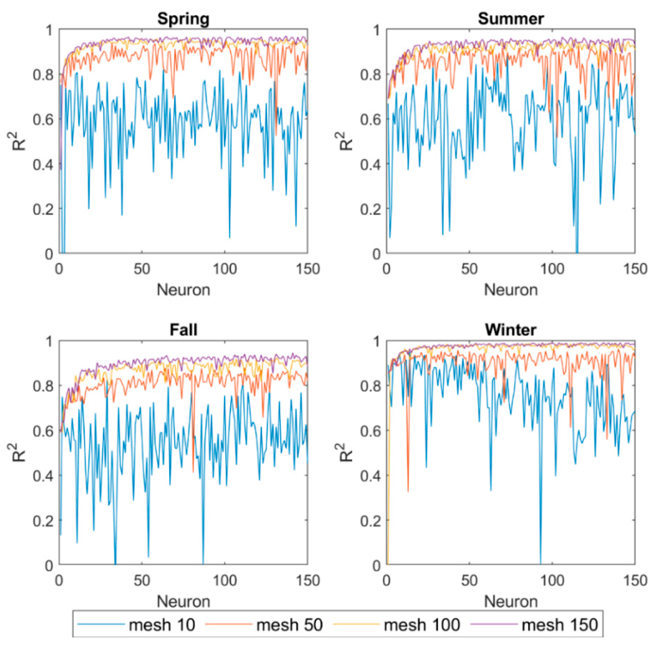
5.4. ANN Model Architecture

The artificial neural network model was built using the Levenberg–Marquardt backpropagation algorithm, as described in the methodology section. A feed-forward neural network with one hidden layer was coded in MATLAB version 9.4 to determine the relationship between input and target. Adding more hidden layers may result in a lower error, but a rigorous method to prevent overfitting was required. All the datasets, including input and output, were normalized to [0,1] prior to model training by subtracting the data from the minimum and dividing by the difference between the minimum and maximum. For a reasonable PM2.5 level prediction, the best grid size, and the optimal number of neurons must be determined, which is crucial to avoid the ANN model under-training or over-fitting [19]. To this end and to study the model’s spatial dependency, data were processed in different grid sizes ranging from 10 to 150 in each direction. Moreover, neurons ranging from one to 150 were examined in each layer. The coefficient of determination (${\mathrm{R}}^2$) was used as an indicator to find the best number of neurons and grid size. Figure 5 presents the variation of ${\mathrm{R}}^2$ and the number of neurons with respect to different grid sizes. Only four representative grid sizes were selected for graphing to avoid overcrowding the figure. According to Figure 5, the grid size of 150 by 150 had the highest ${\mathrm{R}}^2$ value for all seasons, but any grid size above 100 was within a 1.8% margin of error. Generally, a larger grid size generates data at a higher spatial resolution and improves modeling accuracy. Additionally, the ${\mathrm{R}}^2$ was nearly constant for the number of neurons larger than 50. The optimum number of neurons for each of the four seasons was determined as 130. Although increasing the number of neurons in layers could improve accuracy, it would reduce the computational efficiency. Compared with previous research, in which the optimal number of neurons was less than 10 [19], this project adopts a larger number of neurons. The reason why a large number of neurons did not cause over-fitting (based on the test data presented later) in this case is due to the large size of the input dataset.

5.5. ANN Model Performance

After deciding on the optimal number of neurons and grid size, the ANN model was run with the input layer consisting of AOD and meteorological variables. The available datasets were randomly split into three categories of training (70%), validation (15%), and testing (15%) [24]. The performance criteria including coefficient of determination (${\mathrm{R}}^2$), root mean square error (RMSE), and mean absolute percentage error (MAPE) [22] were selected to measure the goodness of fit between the ANN results and the PM2.5 generated by MOVES.

The resulting values of ${\mathrm{R}}^2$, RMSE, and MAPE for the training, validation, and testing periods are reported in

Table 3. The artificial neural network (ANN) model quality assessment using ${\mathrm{R}}^2$, root mean square error (RMSE), and mean absolute percentage error (MAPE).

Season	Year	Train			Validation			Test
		${\mathbf{R}}^2$	RMSE	MAPE	${\mathbf{R}}^2$	RMSE	MAPE	${\mathbf{R}}^2$	RMSE	MAPE
Spring	2010	0.948	0.048	62.96%	0.941	0.052	70.88%	0.949	0.047	67.31%
	2014	0.955	0.044	37.69%	0.943	0.050	41.94%	0.946	0.047	43.58%
	2018	0.952	0.046	41.99%	0.939	0.051	48.94%	0.938	0.053	44.29%
	Mean	0.952	0.046	47.55%	0.941	0.051	53.92%	0.944	0.049	51.73%
Summer	2010	0.954	0.043	63.15%	0.942	0.049	65.33%	0.939	0.052	67.51%
	2014	0.905	0.063	72.69%	0.892	0.067	78.65%	0.870	0.071	79.38%
	2018	0.899	0.065	59.81%	0.874	0.071	63.95%	0.884	0.073	58.27%
	Mean	0.920	0.057	65.21%	0.903	0.062	69.31%	0.897	0.065	68.39%
Fall	2010	0.935	0.052	55.09%	0.928	0.055	57.58%	0.919	0.059	66.09%
	2014	0.947	0.047	42.77%	0.945	0.047	45.12%	0.930	0.053	46.15%
	2018	0.960	0.041	34.89%	0.950	0.048	35.55%	0.948	0.049	40.39%
	Mean	0.947	0.047	44.25%	0.941	0.050	46.08%	0.932	0.054	50.88%
Winter	2010	0.991	0.021	22.65%	0.981	0.032	26.20%	0.985	0.024	25.46%
	2014	0.980	0.030	26.95%	0.977	0.031	28.70%	0.979	0.030	27.81%
	2018	0.980	0.030	26.34%	0.963	0.042	29.34%	0.967	0.039	32.03%
	Mean	0.984	0.027	25.31%	0.974	0.035	28.08%	0.977	0.031	28.44%

. The ${\mathrm{R}}^2$ was considered as the primary index for evaluating model performance. According to Table 3, in the training period, the best model performance was achieved for winter with an average ${\mathrm{R}}^2=0.984$, while more moderate performance was seen in other seasons (spring ${\mathrm{R}}^2=0.952$, fall ${\mathrm{R}}^2=0.947$, and summer ${\mathrm{R}}^2=0.920$). RMSE values closer to zero and lower percentages of MAPE indicate better agreement between the simulated and modeled data. According to a similar study conducted by Yi et al. (2019), MAPE values below 20% were considered good [18]. As shown in Table 3, winter has the lowest MAPE (25.31%) and RSME (0.027) among all seasons. In contrast, the summer MAPE values for the three years of modeling were all above 50%, with the lowest ${\mathrm{R}}^2$ of 0.899 in 2018. Overall, the MAPE values do not represent as good agreement as the ${\mathrm{R}}^2$ values did. This could be due to the large variability of the data that even normalization was not able to resolve.

During the modeling process, ANN backpropagation is prone to over-fitting. When the neural network is so closely fitted to the training data, it is not reliable to make predictions for new data [41]. Validation and testing processes were considered to avoid ANN overfitting. The validation dataset was used for optimizing the model, which stopped the model whenever the error rate was decreased for six consecutive epochs. In addition, a testing dataset was used at the end of the training process to evaluate the overall performance of the model. The performance in validation and testing resembled the results in training. Comparing the ${\mathrm{R}}^2$ values in validation and testing periods, the RMSEs remained below 5% (Table 3). Successful completion of this step proved that the method could replicate standalone case studies. The question remained unanswered: is the model skill in repeating itself, i.e., does the method exhibit seasonality?

The seasonality of the model was investigated by creating four master datasets, each representing one season, e.g., the first master dataset had 2010, 2014, and 2018 spring seasons. To better visualize the model’s performance, a comparison was performed between the ANN simulated and the MOVES estimated PM2.5 values (Figure 6). In this figure, if all the data points were aligned on the 1:1 line (dashed red line), a perfect agreement between the simulated and the modeled values would have been accomplished. Additionally, a line of best fit was shown with a solid black line that did not represent any physical meaning but further highlighted the model bias. As indicated in Figure 6 and discussed before, the winter plot aligned better on the 1:1 line. Some dots deviated from the $1:1$line, significantly affecting RSME and MAPE. This is attributed to either data imperfections or a poor ANN architecture. Perhaps, the inclusion of another hidden layer could resolve this issue. The ${\mathrm{R}}^2$ values listed on top of each subplot were calculated from the master dataset. These values were lower than the ones calculated for each case study reported in Table 3. This decrease was expected because the model is adjusting itself to three years’ worth of data rather than just one case at a time. Nevertheless, the decrease in ${\mathrm{R}}^2$ was in the range of 7 to 12%, compared to the mean correlation highlighted in bold in Table 3. Further, the training, validation, and testing ${\mathrm{R}}^2$ were fairly comparable, confirming that the model was not overfitted.

The other factor affecting the model is the atmospheric pressure, which is positively correlated to particulate matter [14]. As the atmospheric pressure increases, the concentration of various pollutants also increases [14]. Low winds and poor ventilation can cause a higher concentration of air pollutants during high-pressure events. Thus, pressure may be a potential factor affecting the PM2.5 model. The inclusion of atmospheric pressure can be the subject of future research to improve the ANN model. This discussion calls for an analysis of how independent variables are contributing to the outcome.

The relative importance of each independent variable was quantified by conducting a sensitivity analysis on each master dataset [42]. The analysis was performed based on the combined testing, validation, and training datasets. It should be noted that this process was computationally expensive and labor-intensive because of the number and size of the independent variables. The result is presented in

Table 4. Independent variable importance analysis.

		Importance
	Spring	Summer	Fall	Winter
Aerosol Optical Depth	0.20	0.10	0.12	0.12
Precipitation	0.33 *	0.36	0.23	0.24
Temperature	0.09	0.15	0.29	0.16
Relative Humidity	0.24	0.16	0.18	0.30
Wind	0.14	0.23	0.17	0.18

* maximum values in bold.

, where the importance was a value between zero and one, with higher values being more critical in the model performance. Based on these findings, the most important variable was precipitation for summer and spring, temperature for fall, and relative humidity for winter. Precipitation was also the second most important variable in fall and winter, which is why it was one of the emission control methods recommended in the practical applications section of this study. This finding is in agreement with the study conducted by Ouyang et al. 2015 [43].

6. Practical Applications

Particulate matter is a critical air pollutant limited by the Clean Air Act as well as the National Ambient Air Quality Standards (NAAQS). The specific laws and regulations related to emission limitations are crucial for protecting human health and public welfare. Currently, the code of federal regulations (40 CFR Part 86) uses Tier 2 and Interim Non-Tier 2 Full Useful Life Exhaust Mass Emission Standards to regulate PM2.5 emissions for different vehicle types. Additionally, the California Air Resources Board (CARB) Regulations Title 13 covers air quality guidelines for motor vehicles. The model created by this research can assist decision-makers in predicting vehicle PM2.5 emission, develop best management practices, and improve government regulations in controlling emissions.

6.1. Prediction

The models developed in this study can be used to estimate mobile PM2.5 emissions based on meteorological indicators. The model’s input parameters are AOD, temperature, wind speed, precipitation, and relative humidity, all of which are freely available from weather stations. The calibrated ANN model can be coded as a deployable web application capable of generating accurate PM2.5 data. In addition, coupling this model with a climate model such as weather research and forecasting (WRF) [44] will result in particulate matter future forecast. This is possible by using the trained model with the input data generated from a climate model instead of the in-situ and satellite data. The WRF chemistry module (WRF-Chem) [45] is a powerful tool to simulate aerosols in different wavelengths, which is the primary input to the ANN model. This forecast capability makes the model presented here more powerful. With proper trend analysis, more rigorous policies can be adopted to manage the particulate matter levels.

6.2. Best Management Practice

Best management practice (BMP) is a term most associated with water pollution and control systems. This terminology is adopted here to provide recommendations to practitioners. The method developed here can be used as an assessment tool to create multiple air quality forecast scenarios. The recommended scenarios are: (i) impact of car emission control systems, (ii) impact of hybrid or electric vehicles, (iii) impact of alternative fuels, (iv) impact of public transportation, (v) impact of precipitation. These scenarios are analogous with the idea behind the Clean Air Act of (1970) in which there is a significant attempt to reduce the air pollution from vehicle exhaust. Subsequently, it is required to train the ANN model based on new data generated by MOVES for each one of these scenarios. MOVES is customizable to different types of vehicles, fuels, and Clean Air Act regulations. The ANN model trained with these new adjustments will create alternative solutions for state decision-makers. New policies are introduced solely based on these solutions to achieve air pollution attainment. A prominent example of this is the ban on the sales of internal combustion engines in the state of California by 2035 as an attempt to reduce carbon emissions and to adapt to climate change stresses [46].

7. Conclusions

Anthropogenic activities contribute majorly to the presence of PM2.5 in the atmosphere, among which vehicle exhaust emissions account for a large portion, especially in urban areas. This study aimed to develop an ANN model to analyze the relationship between PM2.5 emissions from vehicle exhausts and meteorological variables for the state of California. The spatial data downscaling process was conducted by spatial interpolation using an equal-sized grid over the study domain. The following can be concluded based on this study:

• The pre-modeling evaluation indicated that increasing the grid density improved the accuracy of modeling results significantly.
• The Levenberg–Marquardt backpropagation algorithm with 130 neurons in each layer had the best performance.
• The maximum coefficient of determination was 0.991 for the winter of 2010, and the lowest coefficient of determination of 0.899 was for the summer of 2018, demonstrating the ANN model’s capability in PM2.5 predictions.
• Large variability in the dataset (having both very small and very big values) and the presence of some outliers affected the MAPE values.
• Winter had the best MAPE coefficient, where the possible reason was that winter had the most accurate estimate of AOD for vehicle emission particulate matter.
• Based on the sensitivity analysis, the most important variable among the independent variables was determined to be precipitation.

The analysis performed in this study had some inherent limitations. The MOVES can only estimate the PM2.5 generated from mobile sources. The mass of particulate matter was highly affected by the meteorological indicators in the atmosphere. However, natural emissions are also a large source of PM2.5 in California, and this can degrade the model’s performance during the summer season because of frequent wildfires.

References

1. Roy, S. Prediction of Particulate Matter Concentrations Using Artificial Neural Network. Resour. Environ. 2012, 2, 30–36. [Google Scholar] [CrossRef] [Green Version]
2. Mohebbi, A.; Green, G.T.; Akbariyeh, S.; Yu, F.; Russo, B.J.; Smaglik, E.J. Development of Dust Storm Modeling for Use in Freeway Safety and Operations Management: An Arizona Case Study. Transp. Res. Rec. 2019, 2673, 175–187. [Google Scholar] [CrossRef]
3. Mohebbi, A.; Yu, F.; Cai, S.; Akbariyeh, S.; Smaglik, E.J. Spatial study of particulate matter distribution, based on climatic indicators during major dust storms in the State of Arizona. Front. Earth Sci. 2020, 1–18. [Google Scholar] [CrossRef]
4. Grgurić, S.; Križan, J.; Gašparac, G.; Antonić, O.; Špirić, Z.; Mamouri, R.; Christodoulou, A.; Nisantzi, A.; Agapiou, A.; Themistocleous, K.; et al. Relationship between MODIS based aerosol optical depth and PM10 over Croatia. Open Geosci. 2014, 6, 2–16. [Google Scholar] [CrossRef]
5. Mohebbi, A.; Chang, H.I.; Hondula, D. WRF-Chem Model Simulations of Arizona Dust Storms. In Proceedings of the AGU Fall Meeting Abstracts, New Orleans, LA, USA, 11–15 December 2017. [Google Scholar]
6. Mohebbi, A.; Akbariyeh, S. Geographically Weighted Regression Analysis of Particulate Matter Levels during Major Dust Storms. In Proceedings of the Association of Environmental Engineering and Science Professors (AEESP), Tempe, AZ, USA, 14–16 May 2019. [Google Scholar]
7. Akbariyeh, S.; Patterson, B.M.; Kumar, M.; Li, Y. Quantification of vapor Intrusion pathways: An integration of modeling and site characterization. Vadose Zo. J. 2016, 15. [Google Scholar] [CrossRef]
8. Wang, T.; Zhao, B.; Liou, K.N.; Gu, Y.; Jiang, Z.; Song, K.; Su, H.; Jerrett, M.; Zhu, Y. Mortality burdens in California due to air pollution attributable to local and nonlocal emissions. Environ. Int. 2019, 133, 105232. [Google Scholar] [CrossRef] [PubMed]
9. Jaffe, D.; Hafner, W.; Chand, D.; Westerling, A.; Spracklen, D. Interannual variations in PM2.5 due to wildfires in the Western United States. Environ. Sci. Technol. 2008, 42, 2812–2818. [Google Scholar] [CrossRef] [PubMed]
10. McCarthy, M.C.; Eisinger, D.S.; Hafner, H.R.; Chinkin, L.R.; Roberts, P.T.; Black, K.N.; Clark, N.N.; McMurry, P.H.; Winer, A.M. Particulate matter: A strategic vision for transportation-related research. Environ. Sci. Technol. 2006, 40, 5593–5599. [Google Scholar] [CrossRef] [PubMed] [Green Version]
11. USEPA. Environmental Protection Agency. User Guide for MOVES2014. EPA Report; EPA-420-B-14-055; Office of Transportation and Air Quality: Ann Arbor, MI, USA, 2014.
12. Pauzi, H.M.; Abdullah, L. Airborne particulate matter research: A review of forecasting methods. J. Sustain. Sci. Manag. 2019, 14, 189–227. [Google Scholar]
13. Reid, S.; Bai, S.; Du, Y.; Craig, K.; Erdakos, G.; Baringer, L.; Eisinger, D.; McCarthy, M.; Landsberg, K. Emissions modeling with MOVES and EMFAC to assess the potential for a transportation project to create particulate matter hot spots. Transp. Res. Rec. 2016, 2570, 12–20. [Google Scholar] [CrossRef]
14. Gupta, P.; Christopher, S.A. Particulate matter air quality assessment using integrated surface, satellite, and meteorological products: Multiple regression approach. J. Geophys. Res. Atmos. 2009, 114. [Google Scholar] [CrossRef] [Green Version]
15. Kamarul Zaman, N.A.F.; Kanniah, K.D.; Kaskaoutis, D.G. Estimating Particulate Matter using satellite based aerosol optical depth and meteorological variables in Malaysia. Atmos. Res. 2017, 193, 142–162. [Google Scholar] [CrossRef] [Green Version]
16. Enotoriuwa, R.; Nwachukwu, E.; John, U. Spatial interpolation and land use regression modelling of air. In Proceedings of the 18th International HSE Biennial Conference on the Oil & Gas Industry in Nigeria, Lagos, Nigeria, 26–28 November 2018; pp. 136–148. [Google Scholar]
17. Wu, Y.; Guo, J.; Zhang, X.; Tian, X.; Zhang, J.; Wang, Y.; Duan, J.; Li, X. Synergy of satellite and ground based observations in estimation of particulate matter in eastern China. Sci. Total Environ. 2012, 433, 20–30. [Google Scholar] [CrossRef] [PubMed]
18. Yi, L.; Mengfan, T.; Kun, Y.; Yu, Z.; Xiaolu, Z.; Miao, Z.; Yan, S. Research on PM2.5 estimation and prediction method and changing characteristics analysis under long temporal and large spatial scale—A case study in China typical regions. Sci. Total Environ. 2019, 696, 133983. [Google Scholar] [CrossRef] [PubMed]
19. Memarianfard, M.; Hatami, A.M. Artificial neural network forecast application for fine particulate matter concentration using meteorological data. Glob. J. Environ. Sci. Manag. 2017, 3, 333–340. [Google Scholar]
20. Mohebbi, A.; Maruf, M.; Roubik, J.; Akbariyeh, S. Climate Change Impacts on Precipitation in Arid Regions: An Arizona Case Study. In Proceedings of the AGU Fall Meeting Abstracts, Washington, DC, USA, 10–14 December 2018. [Google Scholar]
21. Wu, Z.; Fan, J.; Gao, Y.; Shang, H.; Song, H. Study on Prediction Model of Space-Time Distribution of Air Pollutants Based on Artificial Neural Network. Environ. Eng. Manag. J. 2019, 18, 1575–1590. [Google Scholar] [CrossRef]
22. Vakili, M.; Sabbagh-Yazdi, S.R.; Khosrojerdi, S.; Kalhor, K. Evaluating the effect of particulate matter pollution on estimation of daily global solar radiation using artificial neural network modeling based on meteorological data. J. Clean. Prod. 2017, 141, 1275–1285. [Google Scholar] [CrossRef]
23. Hagan, M.T.; Demuth, H.B.; Beale, M.H. Neural Network Design; PWS Publishing Co.: Boston, MA, USA, 1996. [Google Scholar]
24. Beale, M.H.; Hagan, M.T.; Demuth, H.B. Neural network toolbox. User Guid. MathWorks 2010, 2, 13–390. [Google Scholar]
25. Allen, J.O.; Mayo, P.R.; Hughes, L.S.; Salmon, L.G.; Cass, G.R. Emissions of size-segregated aerosols from on-road vehicles in the Caldecott Tunnel. Environ. Sci. Technol. 2001, 35, 4189–4197. [Google Scholar] [CrossRef]
26. Li, X.; Dallmann, T.R.; May, A.A.; Stanier, C.O.; Grieshop, A.P.; Lipsky, E.M.; Robinson, A.L.; Presto, A.A. Size distribution of vehicle emitted primary particles measured in a traffic tunnel. Atmos. Environ. 2018, 191, 9–18. [Google Scholar] [CrossRef]
27. Bishop, G.A. Three decades of on-road mobile source emissions reductions in South Los Angeles. J. Air Waste Manage. Assoc. 2019, 69, 967–976. [Google Scholar] [CrossRef] [PubMed]
28. FEAT Fuel Efficiency Automobile Test Data Center. Available online: http://www.feat.biochem.du.edu/light_duty_vehicles.html (accessed on 12 October 2020).
29. Vallamsundar, S.; Lin, J. Overview of US EPA new generation emission model: MOVES. Int. J. Transp. Urban Dev. 2011, 1, 39. [Google Scholar]
30. Guensler, R.; Liu, H.; Xu, Y.; Akanser, A.; Kim, D.; Hunter, M.P.; Rodgers, M.O. Energy consumption and emissions modeling of individual vehicles. Transp. Res. Rec. 2017, 2627, 93–102. [Google Scholar] [CrossRef]
31. EPA. Population and Activity of On-Road Vehicles in MOVES2014; United States Environmental Protection Agency: Washington, DC, USA, 2016.
32. NASA Multi-Angle Implementation of Atmospheric Correction. Available online: https://modis-land.gsfc.nasa.gov/MAIAC.html (accessed on 20 January 2020).
33. Lyapustin, A.; Wang, Y. MCD19A2 MODIS/Terra+Aqua Land Aerosol Optical Depth Daily L2G Global 1km SIN Grid V006 [Data set]. Available online: https://doi.org/10.5067/MODIS/MCD19A2.006 (accessed on 20 January 2020).
34. Wolfe, R.E.; Roy, D.P.; Vermote, E. MODIS land data storage, gridding, and compositing methodology: Level 2 grid. IEEE Trans. Geosci. Remote Sens. 1998, 36, 1324–1338. [Google Scholar] [CrossRef] [Green Version]
35. CIMIS California Irrigation Management Information System. Available online: https://cimis.water.ca.gov/ (accessed on 20 January 2020).
36. DMV California Department of Motor Vehicle, Estimated Vehicles Registered by County for the Period of January 1 through December 31, 2019. Available online: https://www.dmv.ca.gov/portal/uploads/2020/06/2019-Estimated-Vehicles-Registered-by-County-1.pdf (accessed on 2 September 2020).
37. Ramos, É.M.S.; Bergstad, C.J.; Nässén, J. Understanding daily car use: Driving habits, motives, attitudes, and norms across trip purposes. Transp. Res. part F traffic Psychol. Behav. 2020, 68, 306–315. [Google Scholar] [CrossRef]
38. Baith, K.; Lindsay, R.; Fu, G.; McClain, C.R. Data analysis system developed for ocean color satellite sensors. Eos, Trans. Am. Geophys. Union 2001, 82, 202. [Google Scholar] [CrossRef]
39. Brown, J. Governor Brown Announces Federal Approval of Presidential Major Disaster Declaration for Shasta County. Off. Gov. 2018, 32, 309. [Google Scholar]
40. Yang, J.; Hu, M. Filling the missing data gaps of daily MODIS AOD using spatiotemporal interpolation. Sci. Total Environ. 2018, 633, 677–683. [Google Scholar] [CrossRef]
41. Skalski, P. Preventing Deep Neural Network from Overfitting. Available online: https://towardsdatascience.com/preventing-deep-neural-network-from-overfitting-953458db800a (accessed on 17 September 2020).
42. Vashist, R.; Garg, M.L. Computing the Significance of an Independent Variable Using Rough Set Theory and Neural Network. Int. J. Res. Eng. Appl. Sci. 2013, 3, 122–136. [Google Scholar]
43. Ouyang, W.; Guo, B.; Cai, G.; Li, Q.; Han, S.; Liu, B.; Liu, X. The washing effect of precipitation on particulate matter and the pollution dynamics of rainwater in downtown Beijing. Sci. Total Environ. 2015, 505, 306–314. [Google Scholar] [CrossRef]
44. Wang, W.; Bruyère, C.; Duda, M.; Dudhia, J.; Gill, D.; Kavulich, M.; Keene, K.; Chen, M.; Lin, H.-C.; Michalakes, J.; et al. User’s Guides for the Advanced Research WRF (ARW) Modeling System Version 3.9; National Center for Atmospheric Research (NCAR): Boulder, CO, USA, 2018. [Google Scholar]
45. Grell, G.A.; Peckham, S.E.; Schmitz, R.; McKeen, S.A.; Frost, G.; Skamarock, W.C.; Eder, B. Fully coupled “online” chemistry within the WRF model. Atmos. Environ. 2005, 39, 6957–6975. [Google Scholar] [CrossRef]
46. CA.gov Governor Newsom Announces California Will Phase Out Gasoline-Powered Cars & Drastically Reduce Demand for Fossil Fuel in California’s Fight Against Climate Change. Available online: https://www.gov.ca.gov/ (accessed on 28 September 2020).
Figure 1. Weather monitoring stations in the study area.
Environments 07 00102 g001
Figure 2. Project overview. PM2.5: particulate matter of size 2.5 µm (PM2.5); CIMIS: California Irrigation Management Information System; MODIS: Moderate Resolution Spectroradiometer; MOVES: Motor Vehicle Emissions Simulator; MAIAC: Multi-Angle Implementation of Atmospheric Correction.
Environments 07 00102 g002
Figure 3. Spatial mesh in various resolutions generated for the state of California.
Environments 07 00102 g003
Figure 4. Schematic view of a feed-forward artificial neural networks.
Environments 07 00102 g004
Figure 5. The variation of R 2 with respect to the number of neurons for grids 10, 50, 100 and 150.
Environments 07 00102 g005
Figure 6. Seasonal performance of the ANN model, four subplots upper left: spring; four subplots upper right: summer; four subplots bottom left: fall; four subplots bottom right: winter. The seasons are generated from the years 2010, 2014, and 2018. The plots represent the training (70%), validation (15%), and test (15%) datasets as well as all three together (100%).
Environments 07 00102 g006