Abstract
Alum shale was mined for oil and uranium production in Kvarntorp, Sweden, 1942–1966. Remnants such as pit lakes, exposed shale and a 100-meter-high waste deposit with a hot interior affect the surrounding environment, with elevated concentrations of, e.g., Mo, Ni and U in the recipient. Today most pit lakes are circumneutral while one of the lakes is still acidic. All pit lakes show signs of sulfide weathering with elevated sulfate concentrations. Mass transport calculations show that for elements such as uranium and molybdenum the western lake system (lake Söderhavet in particular) contributes the largest part. For sulfate, the two western lakes contribute with a quarter each, the eastern lake Norrtorpssjön about a third and a serpentine pond system receiving water from the waste deposit contributes around 17%. Except for a few elements (e.g., nickel 35%), the Serpentine system (including the waste deposit area) is not a very pronounced point source for metal release compared to the pit lakes. Estimates about future water runoff when the deposit has cooled down suggest only a slight increase in downstream water flow. There could possibly be first flush effects when previous hot areas have been reached by water.
1. Introduction
Mining can have a long-term impact on the surrounding aquatic systems and deteriorate water quality. Pit lakes may have lower biodiversity compared to natural lakes due to water composition, but also due to low physical and biological heterogeneity [1]. Drainage from mining waste have different properties depending on the conditions and can be acidic with pH 0–5, circumneutral with pH 6–8 or alkaline with pH 8–12 [2]. There are several examples worldwide where coal mines have had negative impact on the environment, and it is often associated with acid rock drainage (c.f. [3,4,5]). Mining of black shale can also display the same type of problems with acid rock drainage and metal release since black shales in many cases are a source of acidity and trace metals released to the environment (c.f. [6,7,8]). It has been shown that black shale alteration is initiated by oxidation of pyrite and organic matter [9]. Fractures and pores allow oxygenated fluids to penetrate and alter the chemistry, as well as the mineralogy with possible metal release as a consequence. Hydraulic fracturing could enhance these processes. Soils developed on Cambrian black shales in China have shown increased concentrations of Mo, Ca, Sb, Sn, U, V and Ba [10]. It has been found that from deposits of processed black shale mainly the same metals are dispersed as from acid sulfate soils [11].
In the Kvarntorp area, Sweden, faulting has preserved sedimentary rocks, of which alum shale contains up to 20% organic material in the form of kerogen [12]. This black shale also contains trace elements such as nickel and the redox sensitive trace elements molybdenum, uranium and vanadium [13,14]. Its pyrite content of up to 15% enhance acid rock drainage and metal release which can be intensified by exploitation activities (c.f. [15,16,17]). Burned alum shale, called rödfyr in Swedish, is also a concern for arsenic leaching [18].
In natural waters arsenic is mostly found either as mobile arsenite, As(III), or as arsenate As(V), in general with higher mobility as pH increases. Arsenic can nevertheless occur in several oxidation states, −3, 0, +3, +5, and under slightly reducing conditions it is relatively more mobile compared to other oxyanion forming elements. More reducing acidic conditions, however, favour precipitation of sulfide minerals with coprecipitated arsenic. High concentrations of arsenic are therefore not expected in environments with high concentrations of free sulfide [19]. It has been argued that iron is an important determining factor for arsenic and vanadium concentrations in Swedish streams, since both vanadate and arsenate are adsorbed to iron oxides [20]. There are suggestions though, that the release of vanadium in soil and mine tailings is not easily explained by mobilization mechanisms of other metals since they did not find correlations with vanadium and dissolved species of iron, manganese, zinc, lead, chromium or nickel during leaching tests [21].
Except for phosphorite-black shale deposits where concentrations up to 700 mg/kg dw can be found, black shales usually have low uranium concentrations of about 2–4 mg/kg dw [22]. The uranium concentration in the Kvarntorp shale is about 135 mg/kg dw, but with higher concentrations (245 mg/kg dw) in the upper shale unit [12].
Molybdenum is a chalcophile with +4, +5 and +6 as the most important oxidation states in the environment. It can be found in pyrite, which is nevertheless not thought to be the main sink for molybdenum in euxinic sediments. It is suggested that molybdenum is immobilized in some type of Fe-Mo-S structure [23]. Other studies have shown better correlations for the Mo-TOC relationship than for molybdenum and pyrite [24].
Kvarntorp is an example where large-scale alum shale mining has reshaped the landscape and affected the hydrological conditions. In total about 50 Mtonnes of shale was mined [12] resulting in open pits corresponding to about 2.6 km2. Alum shale mining has left traces such as pit lakes and a deposit consisting of shale waste. This study uses a mass transport approach to find sources and evaluate their impact. It also examines the redistribution of trace elements after primary release. Worldwide, black shales are still investigated as resources concerning, e.g., gas extraction (c.f. [25,26]) or metals [27]. A better understanding of the behavior of already exploited areas would be useful in the consideration of new sites and also for their post mining treatment.
2. Materials and Methods
2.1. Area of Study
Scarcity of liquid fuel during World War II led to oil production from alum shale in the Kvarntorp area, about 200 km west of Stockholm (see Figure 1). Two methods were used for oil production. In the first method, shale was mined in open pits and crushed, followed by pyrolysis, which resulted in waste in the form of burned shale with no sulfides left due to release of sulfur dioxide during pyrolysis. Due to the risk of sintering in the ovens, crushed shale with fractions smaller than 5 mm were screened without being pyrolyzed, which means that there is also shale waste containing pyrite. Waste was primarily used for backfilling of the open pits (both ash and fines) but was also dumped on a waste deposit (Kvarntorpshögen) reaching a height of 100 meters, consisting of about 25 Mtonnes and still today has a hot interior. The second method for oil production was the Ljungström method. Holes were drilled through the limestone layer (which worked as insulation) down to the alum shale which was then heated with electrical heaters, and oil was obtained through condensation of the obtained gas. By this method the permeability in the ground increased, leaving an alum shale layer with changed conditions regarding element release. Oil was produced in Kvarntorp from 1942–1966.
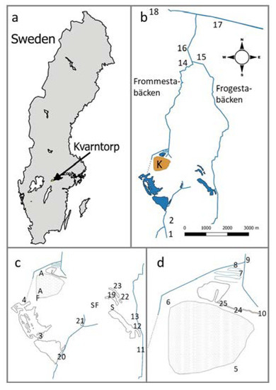
Figure 1.
(a) Location of Kvarntorp; (b) map of the Kvarntorp area. K = waste deposit Kvarntorpshögen, W1, W2, W14, E15, 16 (W + E), 17, 18 = surface water sampling localities (W stands for west and E for east but only the numbers are shown on the map); (c) surface water sampling localities of which some are related to pit lakes, W3 = outlet lake Söderhavet, W4 = outlet lake Nordsjön, E12 = outlet lake Norrtorpssjön, 19 = lake Surpölen, 20 = eastern inlet lake Söderhavet, 21 = lake Mellansjön, 22 = lake Alaborg (south), 23 = lake Alaborg (north). Localities where solid samples were collected are marked with S (shale), F (fines) and A (Shale ash); (d) sampling localities in the waste deposit area, 5 and 6 = stagnant water, W7 = outlet Serpentine pond system, W8 = western stream, W9 = Frommestabäcken where it leaves the Kvarntorp area, 10 = water from the industrial area, 24 = ditch, 25 = ditch.
At the former site for the Ljungström field, there is now a treatment plant for hazardous waste. Some of the open pits have been used for dumping of for instance municipal waste, which means that there are also other point sources than alum shale.
In 2015–2019, an annual precipitation of 501–805 mm was measured in Örebro about 15 km from the Kvarntorp area, according to the Swedish Meteorological and Hydrological Institute [28]. There is no meteorological station in Kvarntorp, but the company Fortum measures the precipitation weekly and reports an annual precipitation of 414–727 mm in 2015–2019. Average annual precipitation in Örebro is 625 mm and average precipitation in the Kvarntorp area is estimated to have been 570 mm during the last 10 years [29], which is thus less than in Örebro. In 2016 and 2018 the precipitation was quite low.
There are two streams in the area (see Figure 1b). The western stream passes two pit lakes before entering a culvert passing west of the deposit. Water from the waste deposit and runoff from the industrial area pass through a passive water cleaning system consisting of a sedimentation pond followed by a serpentine pond system with plants such as phragmites and typha before passing a peat filter. This water is then first joined with clean cooling water from the industrial area before becoming a part of the western stream, which is then called Frommestabäcken. This means that Frommestabäcken is composed of water from lake Söderhavet, lake Nordsjön, the waste deposit area, cooling water and surface runoff from the industrial area. The eastern stream (Frogestabäcken) and Frommestabäcken are joined further north, before reaching a canal leading to lake Hjälmaren.
A major part of the surface water in the area is stored in the pit lakes. Lake Söderhavet (surface area 293,000 m2, average depth 10.5 m) and lake Nordsjön (surface area 411,000 m2, average depth 8 m) together contains about 7 Mm3 [30].
The eastern pit lakes Norrtorpssjön (167,000 m2, depth 5–10 m, 30 m at the deepest part) and Surpölen (31,000 m2, depth 5–15 m) are drained into Frogestabäcken. Two minor lakes (Alaborg, south and north, together 22,000 m2) are drained to the northeast and this water reaches Frogestabäcken further north. Lake Mellansjön (7900 m2) is situated more or less in the center of the area and does not have any apparent surface water outlet but is drained towards lake Söderhavet. Based on the average water flow and lake volumes, the total water turnover time for the western pit lakes is believed to be 1–2 years, and for the eastern lake system 20 years.
In the case of Kvarntorp industrial area, possible remediation strategies have been suggested and debated, but in order to be able to assess environmental impact, further identification of point sources and problem areas is needed. The waste deposit is often the topic for discussions, but a question is whether it is the deposit that is the major source for pollution or not. In this paper, mass transport and element/sulfate ratios calculations are used as an approach to get deeper understanding about the trace element redistribution in a by mining severely affected area.
2.2. Sampling and Analysis
Surface water was sampled monthly from November 2015 to September 2017, and from September 2017 through 2019 every second month. Both upstream localities and downstream localities were chosen, as well as localities in the vicinity of the waste deposit (see Table 1 and Figure 1b–d).

Table 1.
Sampling localities, sampling period and number of sampling occasions.
Within 12 hours of sampling, electrical conductivity, pH and alkalinity were measured. After acidification (nitric acid, 1% final concentration) element concentrations were analyzed using ICP-MS (Agilent 7500cx). Elements prone to suffer from di- and polyatomic interferences (i.e., V, Fe and As) were analyzed in collision mode with helium as the inert collision gas. Anions were analyzed with capillary electrophoresis using sodium chromate buffer (50 mM) containing TTAB (5 mM) and a silica capillary (from 2015 to 2017) or by ion chromatography, SS-EN ISO 10304-1:2009 (from 2018 and onwards).
During sampling, water flow at six localities, W1, W2, W9, W14, E11 and E15 (W stands for west and E for east, in some figures only the numbers are displayed), was estimated using a mechanical current meter with propeller, Eijkelkamp 2030R. There is also a monitoring programme run by Kumla municipality with sampling six times per year at 5–6 localities (corresponding to localities W1, W7, W9, E11, E12 and E13 in this study). For some of these localities water flow is measured continuously and reported on an annual basis (Kumla kommun, 1993–2019). For annual mass transport estimates in 2016, calculations are made using water flow estimates and concentrations from the sampling occasions (method 1). For annual mass transport estimates in 2016–2019, water flow calculations based on the results from Kumla municipality were extrapolated to other localities based on the size of catchment area for each locality. This resulted in an estimated annual water flow, which was used in combination with average annual concentrations to get annual mass transport approximations (method 2). For 2016, results from the two methods are compared.
The formula E = 221.5 + 29.0 T, where E is total evaporation (mm) and T the annual average temperature (°C) can be used for surface runoff calculations [31]. In this paper it has been used to estimate future water runoff from the waste deposit.
In 2017 the eastern pit lakes were sampled in a campaign as previously reported [32], and the western pit lakes were sampled in June 2018. Water was retrieved from different depths in both lake Nordsjön and lake Söderhavet.
Representative solid samples of shale, fines and shale ash (2 samples respectively) were collected in 2019 in the Kvarntorp area (see Figure 1c). Waste materials are relatively homogenous at the site and around 10 kg were collected and homogenized before subsamples were analyzed. In addition, two samples of alkaline materials (autoclaved aerated concrete) were also collected in the area. From each sample a representative amount corresponding to 200 g dw was put in a plastic bottle. In the first step, 400 mL of deionized water (L/S 2) was added. The bottles were shaken intermittently for 24 hours and then the water was removed and analyzed for electrical conductivity, pH, alkalinity, element concentration and anions as described for surface water above. In the second step, 1600 mL deionized water (L/S 8) was added for another period of 24 hours. After that the water was analyzed as in step 1.
Drill cores from the 1940s, with alum shale from the area, kept by the Swedish Geological Survey were also sampled. Solid samples (drill cores and material from the same sampling points as the leaching tests described above) were sent to MS Analytical (Vancouver) for total element quantification where samples were fused with borate flux in a muffle furnace before the resulting beads were dissolved in dilute mineral acid. For the analysis of major elements, ICP-OES was used (Al, Ca, Fe, K, Mg, Mn, Na and P). Samples were also digested in aqua regia or in a 4-acid mixture and analyzed with respect to trace elements (As, Cd, Co, Cu, Mo, Ni, Pb, U and V) by ICP-MS. Total sulfur and carbon were quantified by a Leco carbon and sulfur analyzer.
Principal component analysis (PCA) was performed using the software Unscrambler X version 10.5 (Camo Software AS, Oslo, Norway). Only analytical data from 2019-05-09 were used as this was the sampling occasion containing data from all sampling points (except for localities 5 and 17). Analysis was performed using the following parameters: pH, alkalinity, Cl−, SO42−, Li, Na, K, Rb, Mg, Ca, Sr, Ba, Al, Fe, Mn, As, Cd, Co, Cr, Cu, Mo, Ni, Pb, U and V. All concentration data (except pH) were log-transformed prior to calculation. Map data from Lantmäteriet (Swedish Land Survey) were used in order to process maps and make area calculations with the software QGIS Desktop 2.14.13.
3. Results and Discussion
Analyses of alum shale drill cores, shale from outcrops, fines and shale ash show that iron and sulfur concentrations are lower in shale from outcrops and fines than in unweathered drill cores (Table 2). The higher iron concentrations in shale ash compared to unburned material are due to loss of other elements (such as carbon and sulfur) during the pyrolysis. The total analyses also reveal the heterogeneity of the materials since, for example, shale ash 50 has a calcium concentration of 20,000 mg/kg dw, whereas shale ash 42 only has 2300 mg/kg dw.
Table 2.
Total concentrations (mg/kg dw) in solid samples.
Concentrations and water chemistry in the area show a great range when different localities are compared (e.g., pH median span from 3.26–7.89, sulfate 27–2190 mg/L, uranium 0.2–42.2 µg/L, see Table 3).
Table 3.
Median pH, electrical conductivity, alkalinity, chloride, sulfate and element concentrations in surface water.
3.1. Upstream Versus Downstream Concentrations
A comparison between upstream and downstream water shows higher concentrations for several elements in water that leaves the area than upstream—both in the western and the eastern systems. In the western system concentrations are higher at the outlet than upstream the lakes. Concentrations are also elevated in water that has passed the deposit area. Moreover, in the eastern system water leaving the pit lakes affects the downstream water.
For U, Ni and Mo, elements that all are characteristic for alum shale, the concentrations are higher downstream than upstream (see Figure 2), but for vanadium this is not the case. Even though vanadium is enriched in alum shale, downstream water shows lower concentrations than upstream. Strontium, sulfate and calcium, indicating weathering and buffering reactions, display higher concentrations downstream while alkalinity is lower downstream than upstream. Lithium shows concentration increase as the water passes the alum shale affected area. The pH is generally above 7 both upstream and downstream. Water entering the serpentine system is slightly acidic (see Table 3, localities 24 and 25) and at the serpentine pond outlet median pH is 6.87.
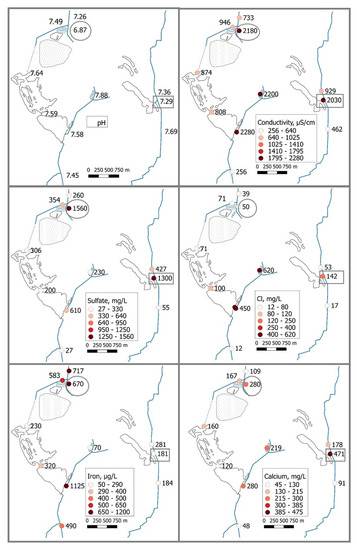
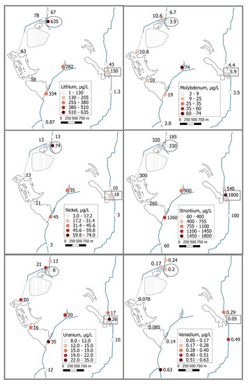
Figure 2.
Median concentrations in surface water November 2015–November 2019 (n = 33–37 except for lake Mellansjön and the eastern inlet of lake Söderhavet where n = 1). Encircled values correspond to concentrations at the serpentine system outlet and values in rectangles show the outlet of lake Norrtorpssjön. For names of localities, see Figure 1c,d.
3.2. Localities Around the Waste Deposit
A ditch north of the waste deposit is believed to receive water from the deposit area (Figure 1d, localities 24, 25). In the ditch, elevated concentrations of sulfate (170–1500 mg/L), U (3–40 µg/L), Li (18–550 µg/L), and Ni (28–274 µg/L) are found. Temperature measurements indicate outflow of water from the warm parts of the deposit. Electrical conductivity measurements also support the idea of leachate water reaching the ditch. From the ditch the water leaves the area by passing an artificial lake and serpentine pond system, created in the end of the 1940s to prevent obvious pollution (based on visible observations and odor) downstream.
Stagnant water northwest of the deposit (Figure 1d, locality 6) also shows influence from alum shale material (98 µg/L uranium, 3500 mg/L sulfate and 400 µg/L molybdenum).
3.3. Piper Diagram and PCA
A Piper diagram with localities around the deposit, pit lakes, upstream waters and downstream waters is presented in Figure 3. Some pit lakes show strong influence from sulfate rich mine drainage and so do some of the localities around the deposit. Upstream localities show calcium bicarbonate waters. The principal components analysis (Figure 4) indicates that the acid pit lake (lake Surpölen, locality 19), plots near the ditch leading from the industrial area (locality 10) past the waste deposit (localities 24 and 25), indicating a strong influence from acid rock drainage at these localities. Lake Norrtorpssjön (locality E12) plots near the outlet from the serpentine ponds (locality W7). Upstream waters (localities W1, W2, E11) and the pit lakes in Alaborg (localities 22, 23) are distinguished from the other localities, thus representing unaffected waters. Trace elements (except for uranium) seem to be related to manganese, iron and aluminum while having a negative association to pH. This can possibly indicate that they are associated to particles (Mn, Fe and Al) where sorption is controlled by pH. Nickel displays a slightly more conservative behaviour compared to the other divalent trace elements. Uranium plots near sodium, potassium, calcium and sulfate. In the PCA, molybdenum is closely related to chloride, indicating a more conservative behavior compared to the other trace elements. Molybdenum sorption is highly influenced by pH, with greatest adsorption at acidic pH [33,34,35]. pH regimes found in Kvarntorp surface waters are thus generally not favourable for molybdenum sorption.
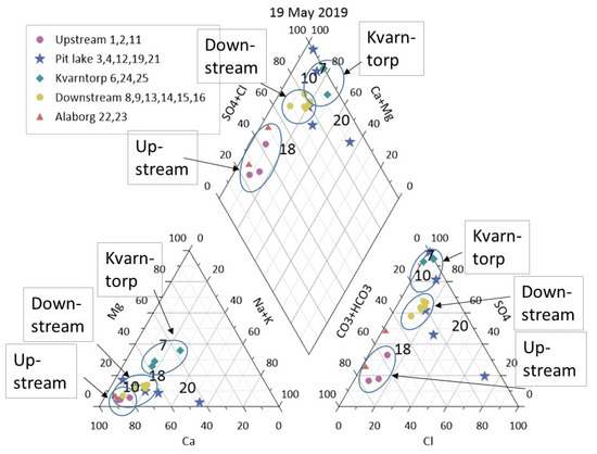
Figure 3.
Piper diagram showing all localities (except 5 and 17) in the Kvarntorp area.
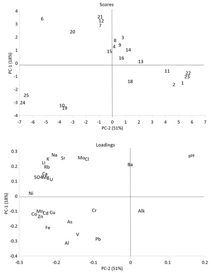
Figure 4.
Principal component analysis (PCA) based on samples from all surface water localities sampled on 9 May 2019. Concentrations are normalized and log-transformed prior to calculations. The first two principal components explain 69% of the total variation in the data. Localities W1, W2, E11, 18, 22 and 23 all represent samples unaffected by the alum shale while localities 10, 19, 24 and 25 all represent samples affected by acid rock drainage.
3.4. Pit Lakes
As can be seen in Table 3, most surface waters are circumneutral. Of the pit lakes (Figure 1c) only one lake, lake Surpölen (locality 19), is acidic today. Lake Surpölen has, however, a higher pH a couple of meters down, indicating either buffering towards the depths or poor mixing of acidic leachates reaching the lake from the oxidising shale horizon surrounding it. Lake Norrtorpssjön (locality E12) was acidic but dumping of alkaline waste in an adjacent municipal waste deposit led to increased pH [32]. Moreover, lake Söderhavet and lake Nordsjön have been acidic during the 1970s. Limestone presence and alkaline waste (lime and autoclaved aerated concrete) could also in these cases be part of the explanation for the neutralization. Alkaline waste dumped near lake Mellansjön (locality 21) is also clearly visible. Water at the outlet of both lake systems (western and eastern) show higher concentrations of elements such as Mo, Ni, Sr and U than background levels, which indicates that the water quality in the lakes is affected by alum shale (c.f. Figure 4).
High chloride concentrations in lake Norrtorpssjön are presumably due to leaching of mixed industrial and household waste, deposited 1985–2008 in an old open pit situated between lake Surpölen and lake Norrtorpssjön. Lake Söderhavet also receives water from a hazardous waste treatment plant and possibly also from lake Mellansjön, which could explain the higher chloride concentrations in lake Söderhavet compared to lake Nordsjön where concentrations are somewhat diluted. Water chemistry is not very different in lake Nordsjön (locality W4) compared to lake Söderhavet (locality W3) as shown in the PCA (Figure 4). This is probably due to the fact that the water turnover is rapid (around 1.5 years) and water from lake Söderhavet is dominating the water in lake Nordsjön. It is not clear why the concentrations of chloride are that elevated in lake Mellansjön. Possibly dumped waste could be the source, but the reason remains uncertain. Depth profiles of chloride in lake Nordsjön and lake Söderhavet (Figure 5) indicate poor mixing with chloride mainly found in the upper parts of the water column. Further, in lake Norrtorpssjön, mixing is expected to be poor, but there the highest chloride concentrations are found deeper down in the water column, which is explained by the chloride containing leachates entering the pit lake through an underground tunnel, and not through surface water.
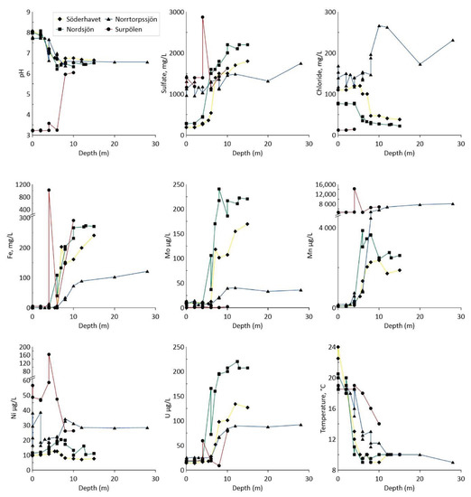
Figure 5.
Depth profiles for pH, sulfate, chloride, Fe, Mo, Mn, Ni, U and temperature in pit lakes. Note changes in the y-axis for iron, manganese and nickel.
Depth profiles in the four major pit lakes indicate reductive dissolution of sorbent phases (mainly iron(III)oxyhydroxides) towards the depth. Electrical conductivity follows the pattern for sulfate quite well. Arsenic, molybdenum, uranium and vanadium have their highest concentrations in the deep water (about 200 µg/L uranium for lake Nordsjön) indicating a release through reductive dissolution of iron and manganese oxyhydroxides. Molybdenum is known to be affected by the manganese cycle [36], which can also be noted in Figure 5. At depths exceeding 10 m, pH seems to converge towards around 6.5 in the four pit lakes. Possibly higher pH at the surface in the circumneutral lakes is connected to photosynthesis and uptake of protons, while further down respiration and decay lowers the pH. For lake Surpölen, one sample at 4 m depth showed high concentrations for several elements, as well as for electrical conductivity. The explanation does not seem to be particles, but the reason for the anomaly remains to be determined.
3.5. Mass Transport
A total annual water flow of 2.5–5.98 Mm3 for 2015-2019 was measured at the outlet of lake Nordsjön (W4) by Kumla municipality (see Table 4 for water flow, precipitation and temperature, Table 5 for estimated catchment areas and Figure 6 for a map of the catchment areas). Downstream the waste deposit (W9), where water from the deposit area (water from the serpentine system W7, 0.17–0.4 Mm3 in 2015–2019) and cooling water from the industrial area (1.198–1.258 Mm3 in 2015–2019 having low concentrations compared to the streams, e.g., Ni 0.5 µg/L, U 0.37 µg/L and sulfate 6.9 mg/L) is joined with water from the western lake system, the annual water flow is estimated to have been 3.93–7.5 Mm3 in 2015–2019 (giving an average of 125–238 L/s) [29]. Since the waste deposit water is part of the serpentine water which constituted 3.6–9.7% of the downstream flow in 2015–2019, the contribution of water coming from the waste deposit area to the downstream volume leaving the area should be less than that range.
Table 4.
Water flow, precipitation and temperature 2015–2019.
Table 5.
Catchment areas.
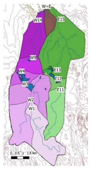
Figure 6.
Map of catchment areas.
For locality W9 and some of the localities where water flow is not measured in the monitoring programme, water flow has been estimated during sampling. By this method 4.3 Mm3 is expected to have passed locality W9 in 2016, which is in very good agreement with calculations made by Kumla municipality (4.33 Mm3). There is not always such a good correlation, since in 2018, for example, Kumla municipality found 5.16 Mm3 and water flow estimates during sampling resulted in 4 Mm3.
Mass transport calculations for 2016 based on water flow estimates during sampling differ slightly for some elements when compared to annual water flow based on continuous measurements extrapolated to other localities (locality E11 0.54/0.56 kg V) and more for other elements (95/55 kg Ni for locality W14). The span for estimated annual mass transport is shown in Table 6.
Table 6.
Annual mass transport, 2016-2019. The span includes differences between the years and results from the different flow estimate methods (locality W1, W2, W9, W14, E11, E15) used in 2016.
Upstream the Kvarntorp area, 40–60 tonnes of sulfate are transported in the streams annually. When the water leaves the lake system (Söderhavet and Nordsjön) it has increased to 700–1000 tonnes and downstream the deposit area 800–1400 tonnes are transported annually. This means that through the lakes 600–1000 tonnes of sulfate is added annually indicating a substantial sulfide weathering. In addition, 260–300 tonnes of sulfate is also added from the Serpentine systems. In the eastern system there is also an addition of sulfate as water from the lakes enters the stream. Annual sulfate fluxes from the area agrees well with, for instance, the sulfate flux (750 tonnes) downstream the Sherritt–Gordon mine in Manotiba, Canada, that was in operation between 1931 and 1951 [38]. The primary sulfide mineral in the alum shale is pyrite (FeS2) according to mineralogical analysis [39,40,41]. Pyrite concentration in the fines is around 12%. Oxidation of pyrite according to the equation below release sulfate and acidity:
2 FeS2 + 7 O2 + 2 H2O => 3 Fe3+ + 4 SO42− + 4 H+
A release of 600–1000 tonnes of sulfate, as in the western lake system, corresponds to a weathering of 400–600 tonnes of pyrite annually equal to 4500–6800 tonnes of fines (assuming 12% pyrite in the fines). During the entire operation between 1942 and 1966, 50 Mtonnes of alum shale were mined and around 20% formed fines. Moreover, 30% of the fines is supposed to have been placed on the waste deposit while the remaining amounts were used for backfilling around the two lakes. At this rate (weathering of 4500–6800 tonnes of fines annually) there are enough fines around the lakes to add the measured amounts of sulfate to the surface waters for a total of 1000–1500 years, if presuming a constant weathering rate. Even though weathering might not be constant, the estimate still gives an idea about the magnitude of weathering potential.
For vanadium and arsenic there is no obvious increase as the water passes the lakes (some years slightly more than upstream and some years slightly less). Molybdenum and uranium concentrations increase as the water passes the lakes, but not necessarily further downstream when the water from the deposit is added (1–4 kg is added from the serpentine system). Lithium transport upstream is about 1–2 kg annually, while it is 100–200 kg at the outlet of the lakes and 270–370 kg downstream the deposit. For lithium, some 100–200 kg is added from the serpentine system. Nickel has the highest concentration at the serpentine system which releases some 10–40 kg annually, contributing to an important part of the total release, possibly due to slightly lower pH than for the other localities [42] and less efficient retention in the serpentine system than for other elements. Figure 7 shows mass transport in 2016 for nickel and uranium calculated with method 2 and with results from method 1 in parentheses.
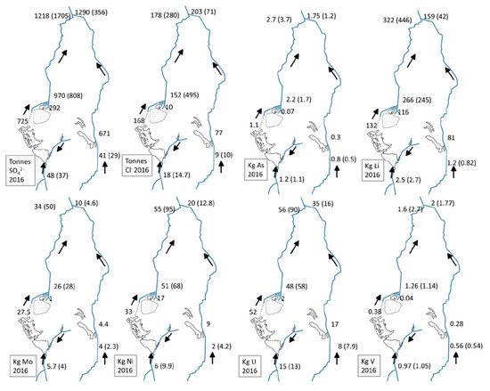
Figure 7.
Estimated mass transport of SO42−, Cl−, As, Li, Mo, Ni, U and V in 2016 calculated with method 2 (results from method 1 in parentheses).
Mass transport added to the water system in the Kvarntorp area would roughly be upstream subtracted from downstream mass transport. For the total area (both the western and the eastern water systems) some 26% of the sulfate is estimated to originate from lake Söderhavet (including lake Mellansjön and water from the waste treatment plant), 24% from lake Nordsjön, 17% from the Serpentine system (including the waste deposit) and 33% from lake Norrtorpssjön. For nickel, lake Söderhavet contributes with 37%, lake Nordsjön 15%, Serpentine system 35% and lake Norrtorpssjön 13%. Chloride mainly originates from lake Söderhavet (including lake Mellansjön) (>75%) and lake Norrtorpssjön (>20%). Moreover, uranium (49%) has the highest contribution from lake Söderhavet (lake Nordsjön 30%, Serpentine system 5% and lake Norrtorpssjön 15%) and half of the molybdenum transport comes from lake Söderhavet (53%, lake Nordsjön 37%, Serpentine system 6%, lake Norrtorpssjön 4%). It does not seem to be any important vanadium release from the lake systems. Some vanadium is released from the serpentine system, but only in small quantities. Leached vanadium is probably redistributed in the water system and in many cases adsorbed and scavenged by iron oxides [20].
3.6. Trace Element/Sulfate Ratios
Since the release of most trace elements from sulfide mining waste are related to the oxidation of sulfides into sulfate their release can be assumed to be related to the release of sulfate [43]. By assuming a conservative behavior for sulfate through the system from release from the waste material to pore waters, groundwaters and further into the surface waters the total amounts of primary released trace elements from the waste materials can be estimated [44]. This is not entirely true, though, as precipitation of sulfate minerals (i.e., gypsum) can remove sulfate from the solutions. As there only are really high sulfate concentrations at L/S 2 during leaching this effect is only expected to give a slight overestimation of the release rates. Results from the leaching tests have been used as a way to determine the trace element/sulfate ratios in leachates from the waste materials (Table 7).
Table 7.
Concentrations, as well as trace element/sulfate ratios (μg/L/mg/L) in leachates from shale (S), fines (F) and shale ash (A) (leached in deionized water).
It is clear that even if the calculated ratios for the different waste materials differ, the ratios for the same type of material are fairly similar (Table 7). It was therefore decided to use average ratios based on the leachates from both L/S 2 and L/S 8 for each waste material. Strontium/sulfate ratios for the alkaline waste material differed compared to the shale waste materials with an average around 7.2 (data not shown). In the western surface water system, it is known that fines, shale and shale ash are present. Average for all waste materials have thus been used in the western system. In the eastern surface water system, there is no known shale ash and therefore only the average for shale and fines has been used. Average trace element/sulfate ratios for the eastern and the western catchment areas are presented in Table 8 below.
Table 8.
Trace element/sulfate ratios (μg/L/mg/L) for upstream and downstream sampling points compared to the average ratios obtained from leaching tests of solid waste materials (shale, fines and shale ash).
By comparing the trace element/sulfate ratios from the waste leaching and the trace element/sulfate ratios in the surface waters (Table 8) a factor indicating how much greater the primary release of trace elements from the waste is compared to the measured mass flow in the surface waters (Table 9). This factor will provide information about to what extent released trace elements from the sub catchment areas are immobilized between the point of release and the surface water. It was not possible to calculate this factor for strontium as the strontium/sulfate ratios were higher in the surface waters compared to the leachates from the shale waste. This indicates that strontium to a large extent originates from the alkaline waste materials.
Table 9.
Theoretical factors indicating how much higher the primary release from the waste materials in the catchment area is compared to the total mass transport in the surface sampling point. Release rates based on the trace elements/sulfate ratios (μg/L/mg/L) (Table 8). It has been assumed that the eastern catchment contains shale, fines and shale ash while the western catchment only contains shale and fines.
In Table 10 below, a comparison between the mass flow in the surface water localities and the assumed release from the sub catchment areas are shown. Calculated mass flow (from trace element/sulfate ratios) are significantly higher than the measured mass flow in the surface waters for all trace elements indicating a significant secondary immobilization within the sub catchment areas. Specific immobilization mechanisms are hard to determine, but secondary immobilization takes place between the release from the waste and the sampling point in the surface waters. A major fraction of the release of trace elements is immobilized on surfaces close to the release through sorption, coprecipitation with iron oxyhydroxides and precipitation [45,46,47]. Immobilization in the pit lakes through sedimentation seems to be minor as the concentrations in the sediments are fairly low as indicated by the concentrations found in pit lake Norrtorpssjön (43 mg/kg dw As, 102 mg/kg dw Mo, 25 mg/kg dw Ni, 86 mg/kg dw U and 68 mg/kg dw V) [32].
Table 10.
Release of trace elements (kg) from the catchment area based on the mass fluxes in surface water sampling points and factors in Table 9 based on trace element/sulfate ratios. Average mass transport has been used for the calculations. Difference between released amounts (calculated) and measured mass flux in the surface waters are assumed to be due to secondary immobilization (adsorption, precipitation, etc.).
pH is, in general, somewhat above neutral, which is ideal for immobilization of cations through sorption. Nickel and zinc have an average immobilization of 96% and 99%, respectively (Table 11), which are fairly expected for these trace elements [45]. Arsenic has an immobilization rate, on average, of 99% indicating coprecipitation with secondary iron minerals [46]. Molybdenum (as molybdate) has, as expected, a lower immobilization rate at around 94%. Uranium also has, on average, a lower immobilization rate (91%), indicating the presence of negative uranyl complexes (carbonate or sulfate for instance) [48]. Calculated secondary immobilization rates for all trace elements are, however, very reasonable considering the pH. Calculated immobilization rates agree well with what have been calculated for other mine sites. A range of 90.1–98.4% for different trace elements was for instance found at the Yorkshire Pennines, UK [44].
Table 11.
Immobilization (%) of the potentially released trace elements from the solid waste in the area. Primary release rates based on the trace elements/sulfate ratios (μg/L/mg/L).
3.7. Water Balance, Waste Deposit
Several factors such as precipitation [49] and vegetation [50] are both important and complex, for water runoff estimates in an area. A crucial question when it comes to the management of the entire Kvarntorp area has been whether or not there will be more runoff generated from the waste deposit in the future when it has cooled down and evaporation due to processes in the deposit decreases. Using Tamm’s formula (without further considerations of vegetation or topography) calculations with an estimated average of 570 mm and average annual temperature estimated to 8 °C results in a runoff around 2 L/s which corresponds to 0.06 Mm3/year if the whole area for the deposit is used in the calculation. A plausible future scenario would be higher temperatures and possibly more precipitation. An average temperature of 10 °C and annual precipitation of 800 mm would generate a runoff of 5 L/s. If the precipitation still is set to 800 mm annually, but a cooler average temperature (5 °C) is considered (not expected according to climate models, but used here to illustrate the maximum of expected runoff), a runoff of 7.5 L/s is calculated, which corresponds to an annual runoff of 0.236 Mm3 from the deposit. Today some of the precipitation received at the deposit is evaporated due to elevated interior temperatures, but not all since the deposit is only partially hot. In 2015–2019 some 0.185–0.4 Mm3 passed the Serpentine system annually (including water from the industrial area and water from the deposit). With a cold deposit this annual amount of water would increase, but with less than the estimated maximum addition of 0.176 Mm3 runoff since far from all precipitation is evaporated today. This means that the amount of water in the downstream recipient (W9) would increase with less than 2–5% since downstream water flow already range between 3.9 and 7.5 Mm3/year. It has previously been estimated [37] that the groundwater recharge for the waste deposit is about 0.5–1 L/s (0.016–0.032 Mm3/year) today and that this could reach 3–5 L/s when the deposit is cold (0.095–0.16 Mm3/year). This means an addition of at most 0.14 Mm3/year compared to today and at most 1.9–3.6% more water in the downstream recipient.
Calculations with Tamm’s formula does not consider seasonal uneven distribution of the precipitation and can therefore only give an idea about the water balance. Nevertheless, it gives an indication of the plausible influence on environmental impact from the deposit. Water balance calculations indicate that the deposit is not by itself necessarily the greatest contributor of leached harmful elements. Estimates of to which extent the waste deposit affects the mass transport are valuable though. Average concentrations in groundwater at the northern rim of the deposit and estimates of current groundwater recharge of 1 L/s results in 86.5 tonnes of sulfate annually, 0.9 tonnes of chloride, 0.9 kg As, 32 kg Li, 3.6 kg Mo, 8 kg Ni, 7.6 kg U and 0.4 kg V. Water from the deposit is believed to pass the Serpentine system which is supposed to have a retaining function and for e.g., uranium the Serpentine system does release less than a quarter of the mass estimated from the deposit, whereas for nickel the release from the Serpentine system is greater than estimates for the deposit. Without considering the Serpentine system, less than 17% of uranium, 10% of sulfate and 16% of nickel downstream west would originate from the deposit.
The amount of water penetrating the deposit is not the only important factor in future mass transport scenarios. Former hot areas, which have not been in contact with water, could show initial first flush effects with increased concentrations in the leachates. As the cooling proceeds there could be overlapping first flush effects, obscuring the different flush events. This means that as the deposit cools, there could be changes in both flow and concentrations in the future.
4. Conclusions
Alum shale mining, oil and uranium production has affected the environment in Kvarntorp. Localities around the waste deposit show elevated concentrations of for example Li, Mo, Ni and U. Downstream water has higher concentrations of these elements than water upstream the Kvarntorp area. Features such as the pit lakes, weathering shale exposures and the waste deposit all affect the downstream water quality, although mining and production ceased more than 50 years ago.
Mass transport calculations have made it possible to identify the most significant sources for sulfate and trace elements to the recipient.
Mass transport estimates give that some 800–1360 tonnes of sulfate, 240–370 kg of Li, 50–120 kg of Ni and 40–60 kg of U leaves the western part of the area annually. Of the elements released to downstream water some 10–40 kg nickel and 100–200 kg lithium come from the serpentine system whereas the transport of other elements seems to be less important (uranium <4 kg). The deposit itself is today likely contributing less than 20% for most elements in downstream water. An increased future release when the deposit cools off could be expected, and possibly with first flush effects, although the amount of increased water reaching the downstream recipient is not predicted to be more than a few percent. In the eastern system lake Norrtorpssjön is estimated to release some 540 tonnes of sulfate, 7 kg of nickel and 8 kg uranium annually.
Sulfate release and trace element sulfate ratios still indicate a significant weathering of pyrite within the catchments. Sulfate is being released into the surface waters and it is estimated that the release will continue for at least 1000–1500 years at the current rate. Trace element/sulfate ratio calculations indicate that while sulfate is being released into the recipient a large fraction of the released trace elements is being immobilized either in secondary minerals or through adsorption.
Author Contributions
K.Å. and M.B. performed the study conception and design. K.Å. performed the regular water sampling and flow measurements, sample preparations and analyses. K.Å. and M.B. performed the sampling in the pit lakes and sampling of solid material. V.S. performed the metal analysis and data interpretation. The first draft was written by K.Å. M.B. wrote the chapter about trace element–sulfate ratios. Supervision was carried out by M.B. All authors commented on previous versions of the manuscript and all authors have read and agreed to the published version of the manuscript.
Funding
This research received no external funding.
Acknowledgments
Kumla municipality is gratefully acknowledged for permitting sampling in the area and for sharing monitoring data. We also would like to thank the Swedish Geological Survey for providing access to the old exploration drill cores from the area.
Conflicts of Interest
The authors declare no conflict of interest.
References
- Luek, A.; Rasmussen, J.B. Chemical, Physical and Biological Factors Shape Littoral Invertabrate Community Structure in Coal-Mining End-Pit Lakes. Environ. Manag. 2017, 59, 652–664. [Google Scholar] [CrossRef] [PubMed]
- Nordstrom, D.K. Mine Waters: Acidic to circumneutral. Elements 2011, 7, 393–398. [Google Scholar] [CrossRef]
- Lattuada, R.M.; Menezes, C.T.B.; Pavei, P.T.; Peralba, M.C.R.; Dos Santos, J.H.Z. Determination of metals by total reflection X-ray fluorescence and evaluation of toxicity of a river impacted by coal mining in the south of Brazil. J. Hazard. Mater. 2009, 163, 531–537. [Google Scholar] [CrossRef] [PubMed]
- Griffith, M.B.; Norton, S.B.; Alexander, L.C.; Pollard, A.I.; LeDuc, S.D. The effect of mountaintop mines and valley fills on the physicochemical quality of stream ecosystems in the central Appalachians: A review. Sci. Total Environ. 2012, 417, 1–12. [Google Scholar] [CrossRef] [PubMed]
- Wright, I.A.; Belmer, N.; Davies, P.J. Coal Mine Water Pollution and Ecological Impairment of One of Australia’s Most ‘Protected’ High Conservation-Value Rivers. Water Air Soil Pollut. 2017, 228, 90. [Google Scholar] [CrossRef]
- Parviainen, A.; Loukola-Ruskeeniemi, K. Environmental impact of mineralised black shales. Earth Sci. Rev. 2019, 192, 65–90. [Google Scholar] [CrossRef]
- Perkins, R.B.; Mason, C.E. The relative mobility of trace elements from short-term weathering of a black shale. Appl. Geochem. 2015, 56, 67–79. [Google Scholar] [CrossRef]
- Yu, C.; Lavergren, U.; Peltola, P.; Drake, H.; Bergbäck, B.; Åström, M.E. Retention and transport of arsenic, uranium and nickel in a black shale setting revealed by a long-term humidity cell test and sequential chemical extractions. Chem. Geol. 2014, 363, 134–144. [Google Scholar] [CrossRef]
- Jin, L.; Mathur, R.; Rother, G.; Cole, D.; Bazilevskaya, E.; Williams, J.; Carone, A.; Brantley, S. Evolution of porosity and geochemistry in Marcellus Formation black shale during weathering. Chem. Geol. 2013, 356, 50–63. [Google Scholar] [CrossRef]
- Yu, C.; Peng, B.; Peltola, P.; Tang, X.; Xie, S. Effect on weathering on abundance and release of potentially toxic elements in soils developed on Lower Cambrian black shales, P.R. China. Environ. Geochem. Health 2012, 34, 375–390. [Google Scholar] [CrossRef]
- Lavergren, U.; Åström, M.E.; Falk, H.; Bergbäck, B. Metal dispersion in groundwater in an area with natural and processed black shale—Nationwide perspective and comparison with acid sulfate soils. Appl. Geochem. 2009, 24, 359–369. [Google Scholar] [CrossRef]
- Andersson, A.; Dahlman, B.; Gee, D.G.; Snäll, S. The Scandinavian Alum Shales; Ser. Ca. No. 56; Sveriges Geologiska Undersökning: Uppsala, Sweden, 1985. [Google Scholar]
- Armands, G. Geochemical studies of uranium, molybdenum and vanadium in a Swedish alum shale. Ph.D. Thesis, Stockholm University, Stockholm, Sweden, 1972. [Google Scholar]
- Buchardt, B.; Thorshøj Nielsen, A.; Schovsbo, N.H. Alun Skiferen i Skandinavien. Geol. Tidsskr. 1997, 3, 1–30. (In Danish) [Google Scholar]
- Puura, E. Weathering of Mining Waste Rock Containing Alum Shale and Limestone: A Case-Study of the Maardu Dumps, Estonia. Ph.D. Thesis, Kungliga Tekniska Hogskolan, Stockholm, Sweden, 1998. [Google Scholar]
- Kalinowski, B.E.; Johnsson, A.; Arlinger, J.; Pedersen, K.; Ödegaard-Jensen, A.; Edberg, F. Microbial Mobilization of Uranium from Shale Mine Waste. Geomicrobiol. J. 2006, 23, 3–4. [Google Scholar] [CrossRef]
- Lavergren, U. Metal Dispersion from Natural and Processed Black Shale. Ph.D. Thesis, University of Kalmar, Kalmar, Sweden, 2008. [Google Scholar]
- Andrén, J. Potentiellt hög Urlakning av Arsenik Till Grundvattnet Från Rödfyrshög i Kinne-Kleva. (Potentially High Arsenic Leaching to the Groundwater from Heap of Rödfyr in Kinne-Kleva). Bachelor’s Thesis, Uppsala University, Uppsala, Sweden, 2016. (In Swedish with abstract in English). [Google Scholar]
- Smedley, P.L.; Kinniburgh, D.G. A review of the source, behavior and distribution of arsenic in natural waters. Appl. Geochem. 2002, 17, 517–568. [Google Scholar] [CrossRef]
- Wällstedt, T.; Björkvald, L.; Gustafsson, J.P. Increasing concentrations of arsenic and vanadium in (southern) Swedish streams. Appl. Geochem. 2010, 25, 1162–1175. [Google Scholar] [CrossRef]
- Yang, J.; Tang, Y.; Yang, K.; Rouff, A.A.; Elzinga, E.J.; Huang, J.-H. Leaching characteristics of vanadium in mine tailings and soils near a vanadium titanomagnetite mining site. J. Hazard. Mater. 2014, 264, 498–504. [Google Scholar] [CrossRef] [PubMed]
- Cumberland, S.A.; Douglas, G.; Grice, K.; Moreau, J.W. Uranium mobility in organic matter-rich sediments: A review of geological and geochemical processes. Earth Sci. Rev. 2016, 159, 160–185. [Google Scholar] [CrossRef]
- Smedley, P.L.; Kinniburgh, D.G. Molybdenum in natural waters: A review of occurrence, distributions and controls. Appl. Geochem. 2017, 84, 387–432. [Google Scholar] [CrossRef]
- Chappaz, A.; Lyons, T.W.; Gregory, D.D.; Reinhard, C.T.; Gill, B.C.; Li, C.; Large, R.R. Does pyrite act as an important host for molybdenum in modern and ancient euxinic sediments? Geochim. Cosmochim. Acta 2014, 126, 112–122. [Google Scholar] [CrossRef]
- Schovsbo, N.H.; Nielsen, A.T.; Gautier, D.L. The Lower Palaeozoic shale gas play in Denmark. Geol. Surv. Denmark Greenland Bull. 2014, 31, 19–22. [Google Scholar] [CrossRef]
- Zhongbao, L.; Bo, G.; Dongjun, F.; Xuehui, C.; Wei, D.; Yang, W.; Donghui, L. Mineral composition of the Lower Cambrian black shale in the Upper Yangtze region and its significance in oil and shale gas exploration. Nat. Gas Ind. B 2017, 4, 340–345. [Google Scholar]
- Hade, S.; Soesoo, A. Estonian Graptolite Argillites Revisited: A Future Resource? Oil Shale 2014, 31, 4–18. [Google Scholar] [CrossRef]
- SMHI. Ladda ner Meteorologiska Observationer. Available online: https://www.smhi.se/data/meteorologi/ladda-ner-meteorologiska-observationer/#param=precipitation24HourSum,stations=all (accessed on 12 February 2020).
- Kumla Kommun. Water Monitoring Program in Kvarntorp; Annual Reports 1993–2019; Kvarntorps Vatten: Örebro, Sweden, 1993. (In Swedish) [Google Scholar]
- Salomonsson, G. (Archive material, Arkivcentrum, Örebro, Sweden). Avledning av ammoniakvatten till Kvarntorpssjöarna, Terra Bona. Unpublished Report. 1970; 30p. (In Swedish) [Google Scholar]
- Tamm, O.F.S. Studier över klimatets humiditet i Sverige. In Bulletin of the Royal School of Forestry; Bulletin of the Royal School of Forestry: Stockholm, Sweden, 1959; Volume 32, p. 50, (In Swedish and German). [Google Scholar]
- Åhlgren, K.; Sjöberg, V.; Grawunder, A.; Allard, B.; Bäckström, M. Chemistry of Acidic and Neutralized Alum Shale Pit Lakes 50 Years after Mine Closure, Kvarntorp, Sweden. Mine Water Environ. 2020, 39, 481–497. [Google Scholar] [CrossRef]
- Johannesson, K.H.; Tang, J. Conservative behavior of arsenic and other oxyanion-forming trace elements in an oxic groundwater flow system. J. Hydrol. 2009, 378, 13–28. [Google Scholar] [CrossRef]
- Schneider, A.B.; Koschinsky, A.; Kiprotich, J.; Poehle, S.; do Nascimento, P.C. An experimental study on the mixing behavior of Ti, Zr, V and Mo in the Elbe, Rhine and Weser estuaries. Estuar. Coast. Shelf Sci. 2016, 170, 34–44. [Google Scholar] [CrossRef]
- Sun, W.; Selim, H.M. Kinetic modeling of molybdenum sorption and transport in soils. Environ. Sci. Pollut. 2020, 27, 20227–20234. [Google Scholar] [CrossRef]
- Bauer, S.; Blomqvist, S.; Ingri, J. Distribution of dissolved and suspended particulate molybdenum, vanadium and tungsten in the Baltic Sea. Mar. Chem. 2017, 196, 135–147. [Google Scholar] [CrossRef]
- Holm, T.; Ekholm, D.; Johansson, L.; Bäckström, M.; Rehn, I.; Forsmark, T.; Axenhamn, L.; Sundblad, B. Kvarntorpsområdet—Studie av Kvarntorpshögen; Report; SWECO VIAK AB and SGU: Gothenburg, Sweden, 2005. (In Swedish) [Google Scholar]
- Monur, M.C.; Ptacek, C.J.; Hayashi, M.; Blowes, D.; Birks, S.J. Seasonal cycling and mass-loading of dissolved metals and sulfate discharging from an abandoned mine site in northern Canada. Appl. Geochem. 2014, 41, 176–188. [Google Scholar] [CrossRef]
- Chi Fru, E.; Hemmingsson, C.; Callac, N.; Perez, N.; Panova, E.G.; Broman, C.; el Albani, A. Atmospheric weathering of Scandinavian alum shales and the fractionation of C, N and S isotopes. Appl. Geochem. 2016, 74, 94–108. [Google Scholar] [CrossRef]
- Lerat, J.G.; Sterpenich, J.; Mosser-Ruck, R.; Lorgeoux, C.; Bihannic, I.; Fialips, C.I.; Schovsbo, N.H.; Pironon, J.; Gaucher, E.C. Metals and radionuclides (MaR) in the Alum Shale of Denmark: Identification of MaR-bearing phases for the better management of hydraulic fracturing waters. J. Nat. Gas Sci. Eng. 2018, 53, 139–152. [Google Scholar] [CrossRef]
- Åhlgren, K.; Sjöberg, V.; Bäckström, M. Leaching of U, V, Ni and Mo from alum shale waste as a function of redox and pH–suggestion for a leaching method. In Mine Water: Risk to Opportunity, Proceedings of the 11th ICARD/IMWA: Pretoria, South Africa, 10–14 September 2018; Wolkersdorfer, C., Sartz, L., Weber, A., Burgess, J., Tremblay, G., Eds.; Tshwane University of Technology: Pretoria, South Africa, 2018; pp. 782–787. [Google Scholar]
- Falk, H.; Lavergren, U.; Bergbäck, B. Metal mobility in alum shale from Öland, Sweden. J. Geochem. Explor. 2006, 90, 157–165. [Google Scholar] [CrossRef]
- Kim, D.-M.; Yun, S.-T.; Cho, Y.; Hong, J.-H.; Batsaikhan, B.; Oh, J. Hydrochemical assessment of environmental status of surface and ground water in mine areas in South Korea: Emphasis on geochemical behaviors of metals and sulfate in ground water. J. Geochem. Explor. 2017, 183, 33–45. [Google Scholar] [CrossRef]
- Jones, A.; Rogerson, M.; Greenway, G.; Potter, H.A.B.; Mayes, W.M. Mine water geochemistry and metal flux in a major historic Pb-Zn-F orefield, the Yorkshire Pennines, UK. Environ. Sci. Pollut. Res. 2013, 20, 7570–7581. [Google Scholar] [CrossRef] [PubMed]
- Matern, K.; Lux, C.; Ufer, K.; Kaufhold, S.; Mansfeldt, T. Removal of nickel from groundwater by iron and manganese oxides. Int. J. Environ. Sci. Technol. 2018, 16, 2895–2904. [Google Scholar] [CrossRef]
- Yang, Z.; Liu, L.; Chai, L.; Liao, Y.; Yao, W.; Xiao, R. Arsenic immobilization in the contaminated soil using poorly crystalline Fe-oxyhydroxy sulfate. Environ. Sci. Pollut. 2015, 22, 12624–12632. [Google Scholar] [CrossRef]
- Xu, N.; Christodoulatos, C.; Braida, W. Adsorption of molybdate and tetrathiomolybdate onto pyrite and goethite: Effect of pH and competitive anions. Chemosphere 2006, 62, 1726–1735. [Google Scholar] [CrossRef]
- Yuan, F.; Cai, Y.; Yang, S.; Liu, Z.; Chen, L.; Lang, Y.; Wang, K.; Wang, S. Simultaneous sequestration of uranyl and arsenate at the goethite/water interface. J. Radioanal. Nucl. Chem. 2017, 311, 815–831. [Google Scholar] [CrossRef]
- Fekete, B.M.; Vörösmarty, C.J.; Roads, J.O.; Willmott, C.J. Uncertainties in Precipitation and Their Impacts on Runoff Estimates. J. Clim. 2004, 17, 294–304. [Google Scholar] [CrossRef]
- Peel, M.C.; McMahon, T.A.; Finlayson, B.L. Vegetation impact on mean annual evapotranspiration at a global catchment scale. Water Resour. Res. 2010, 46, 16. [Google Scholar] [CrossRef]
Publisher’s Note: MDPI stays neutral with regard to jurisdictional claims in published maps and institutional affiliations. |
© 2020 by the authors. Licensee MDPI, Basel, Switzerland. This article is an open access article distributed under the terms and conditions of the Creative Commons Attribution (CC BY) license (http://creativecommons.org/licenses/by/4.0/).