Article

Mixture Probability Distributions for Low-Flow Frequency Analysis in Mexico: Implications for Environmental Impact Assessment, Drought Management, and Regional Water Policy

by
Carlos Escalante-Sandoval
Faculty of Engineering, National Autonomous University of Mexico, Mexico City 04510, Mexico
Environments 2025, 12(12), 450; https://doi.org/10.3390/environments12120450
Submission received: 3 October 2025 / Revised: 12 November 2025 / Accepted: 18 November 2025 / Published: 21 November 2025

Abstract

Reliable estimation of low-flow statistics is essential for water quality regulation, ecological protection, and drought management. This study evaluates traditional univariate and two-component Mixture Probability Distributions for modeling 7-day annual minimum flows (7Q) using records from 293 gauging stations across Mexico’s 37 hydrological planning regions, each with at least 20 years of data. Candidate models include Lognormal-3, Gamma-3, Gumbel, Weibull-3, and mixtures (Gumbel–Gumbel, Gumbel–Weibull-3, Weibull-3–Gumbel, Weibull-3–Weibull-3). Parameters are estimated by maximum likelihood, goodness-of-fit is assessed with Kolmogorov–Smirnov and Anderson–Darling tests. Sampling uncertainty is quantified via nonparametric bootstrap, providing 95% confidence intervals for design return levels, including 7Q10. Mixture models are selected as the best fit at 253 of 293 stations (86.3%), with Weibull-3–Weibull-3 dominating (45.1% of all stations) followed by Gumbel–Weibull-3 and Weibull-3–Gumbel; univariate models account for only 13.7% of cases, mainly Lognormal-3, and Gumbel alone is never preferred. Gumbel-only and symmetric G–G mixtures yield negative low-flow return levels at some sites and are therefore considered physically implausible. In contrast, mixtures containing Weibull-3 components ensure non-negative support, provide superior fit to the lower tail, and generally produce narrower bootstrap confidence intervals than the best univariate alternatives, indicating more stable and defensible 7Q10 estimates and providing an additional criterion to distinguish between models with similar goodness-of-fit statistics. These findings have direct implications for Environmental Impact Assessment, effluent permitting, ecological flow setting, drought planning, and regional water policy. The results support integrating Weibull-based mixtures—especially Weibull-3–Weibull-3 and Gumbel–Weibull-3—into Mexico’s national framework for low-flow frequency analysis and regulatory design.

1. Introduction

Low flows are critical hydrological indicators for maintaining ecological integrity [1,2], regulating effluent discharges, and planning water allocation during scarcity. Among these, the 7-day low flow with a 10-year return period (7Q10) is widely used in water quality standards and drought preparedness frameworks. Accurate estimation of 7Q10 requires probability models that capture the lower tail of streamflow distributions, where traditional families often underperform [3].
Historically, low-flow frequency studies have applied classical univariate distributions [4,5]—such as the Lognormal, Weibull, Gamma, and Gumbel—to annual minima of n-day averaged flows. These models are attractive because they are interpretable, parsimonious, and easy to fit with methods such as moments, L-moments, or maximum likelihood. Several national and regional assessments in Europe and elsewhere confirm that such families can perform adequately for 7Q or Q95 indices [6,7], though their relative performance varies with hydro-climatic regime, record length, and physiographic heterogeneity. In Italy and Austria, for example, regional low-flow studies have emphasized index-flow and regression frameworks to improve robustness where records are short and spatial variability is high. Similar strategies have been developed in the UK and Scandinavia [2,8], linking catchment characteristics to drought and low-flow metrics.
The present work focuses on the 7-day, 10-year low flow (7Q10) rather than percentile-based indicators such as Q95 for three reasons. First, 7Q10 is widely adopted in regulatory practice as a design flow for water quality standards, discharge permitting, and minimum ecological flow requirements, particularly in the United States and Latin America [1,9,10], because it represents a low-flow condition of defined recurrence severity rather than a purely descriptive percentile. Second, the 7-day averaging window explicitly filters out short-lived daily anomalies and instead targets sustained low-flow periods relevant for habitat stress, drinking water intake reliability, and wastewater dilution capacity, whereas single-day minima or high-percentile indices (e.g., Q90, Q95) can be more sensitive to measurement noise and operational releases. Third, in many Mexican basins—especially regulated and drought-prone systems—flow regimes exhibit prolonged recession driven by groundwater depletion and storage management. Under these conditions, the persistence aspect embedded in 7Q10 is more policy-relevant than purely statistical exceedance probabilities. For these reasons, 7Q10 is the quantity most directly usable by agencies that must set enforceable limits and emergency triggers, and it provides a consistent national basis for comparing hydrologic stress across contrasting regions.
Despite the practical success of traditional models, there is growing recognition that single unimodal distributions may fail where hydrologic regimes reflect multiple generating processes—e.g., baseflow–surface flow interactions, regulated reaches with operational shifts, or climates with distinct monsoonal and non-monsoonal dry seasons. In such contexts, finite mixture models—defined as convex combinations of two or more component distributions—can provide improved tail fit and greater flexibility for skewness and kurtosis [5,11,12]. Mixtures have been applied in hydrology to extremes of precipitation, flood peaks, and regime-switching rainfall states, yet their use for low-flow frequency analysis—and particularly for 7Q10 across climatically diverse networks—remains comparatively limited [1,2].
Mexico offers a suitable and highly informative setting to evaluate these methods because of its pronounced hydro-climatic diversity. The country is divided into 37 hydrological planning regions (RHS) [13] that span arid desert basins in the north (e.g., Río Bravo, Mapimí), temperate highland catchments in the central plateau (e.g., Lerma–Santiago, Balsas), humid tropical lowlands in the southeast (e.g., Grijalva–Usumacinta, Papaloapan), and karstic systems in the Yucatán Peninsula. This range of climatic and physiographic conditions produces markedly different low-flow generation mechanisms, from long groundwater recession and reservoir-controlled releases in semi-arid rivers to strong seasonal contrasts in perennial tropical systems. Because these processes coexist within a single national water-planning framework, Mexico provides an operationally relevant testbed for assessing whether mixture distributions offer a robust, transferable alternative to conventional univariate low-flow models.
Beyond statistical interest, improving low-flow modeling has direct environmental and management implications. Underestimation of 7Q10 can result in over-allocation of scarce resources or inadequate protection of aquatic ecosystems, while overestimation may impose unnecessarily strict regulation [1]. In the context of environmental impact assessment and drought management, robust estimation methods are essential to reduce uncertainty and strengthen risk-based planning [2,4].
This study addresses two linked questions. First, can flexible two-component mixture distributions reproduce low-flow behavior across Mexico’s contrasting RHS better than traditional single-family (univariate) models? Second, do these statistical gains matter for management, for example, when estimating the 7Q10 design flow used in permitting, ecological flow definition, drought contingency planning, and basin-scale water allocation? To answer these questions, we analyze 7-day annual low flows (7Q series) from 293 gauging stations with at least 20 years of record, covering all 37 RHS recognized in national water planning. We compare widely used univariate families (Lognormal-3, Gamma-3, Gumbel, Weibull-3) with finite mixtures built from Gumbel and Weibull-3 components. Model parameters are estimated by maximum likelihood, and model selection is based on Kolmogorov–Smirnov and Anderson–Darling tests. By framing the analysis at the national and regional scales used by Mexican water authorities, we link statistical performance directly to regulatory applications such as effluent dilution standards, ecological flow targets, reservoir operation under drought, and regional allocation policies.

2. Materials and Methods

2.1. Study Area

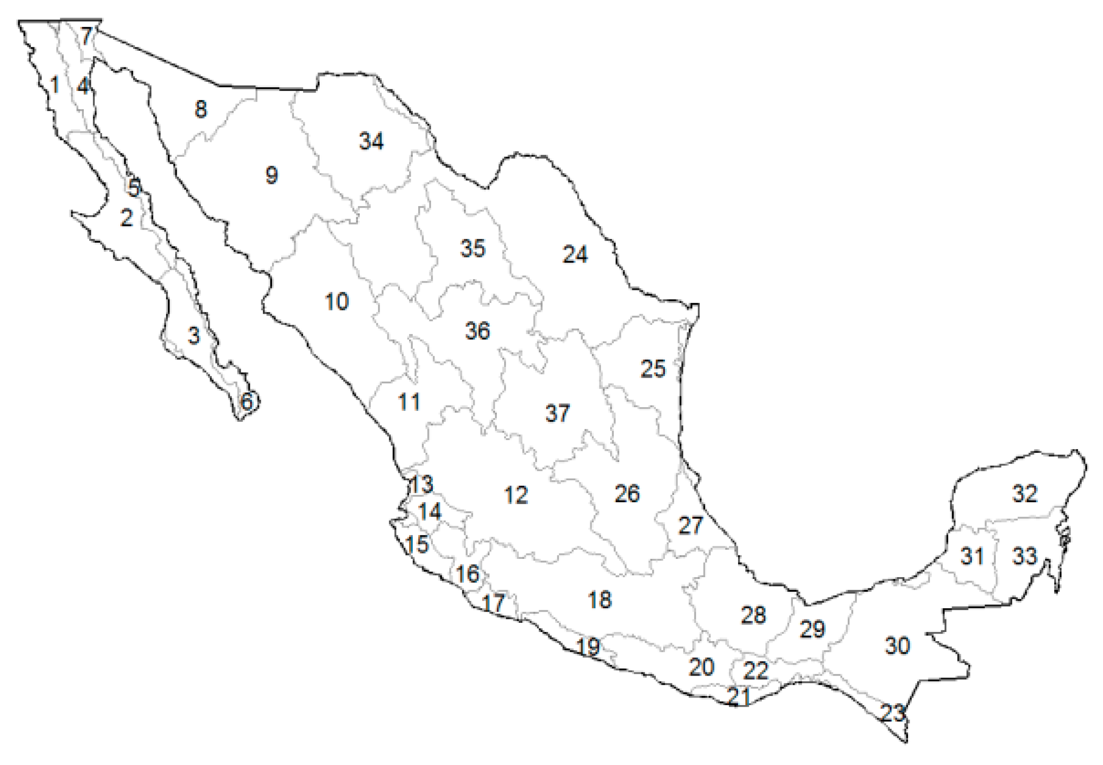
Mexico covers almost 2 million km2 and exhibits pronounced hydro-climatic contrasts, from arid deserts in the north to humid tropical basins in the southeast. This variability is reflected in the 37 RHS of Mexico, officially defined by the National Water Commission (CONAGUA, Mexico) [13], which serve as the basis for national water planning and management (Figure 1, Table 1). Each region integrates climatic, physiographic, and drainage-basin characteristics, providing a consistent framework for analyzing low-flow regimes and for interpreting the results in terms of practical water management needs.
To aid interpretation of national patterns, the 37 RHS were further grouped into four broader hydro-climatic classes used throughout the analysis: (i) northern and northwestern arid regions; (ii) central highlands and transition zones; (iii) Gulf of Mexico basins; and (iv) southern tropical basins. This grouping is process-based rather than purely geographic. It reflects dominant climate drivers (arid/semi-arid vs. humid tropical rainfall regimes), hydrologic controls on baseflow (groundwater-fed recession vs. perennial runoff), and water-use pressures (e.g., intensive regulation and abstraction in Lerma–Santiago and Balsas versus largely perennial, high-yield systems in the Grijalva–Usumacinta). Operationally, we delineated these groups using mean annual precipitation, persistence of dry-season flow, and known management stress (aquifer over-extraction, reservoir operation), and then aligned them with CONAGUA’s planning regions [13]. In other words, the classification links hydrologic behavior to the actual institutional units used for water allocation and drought planning.
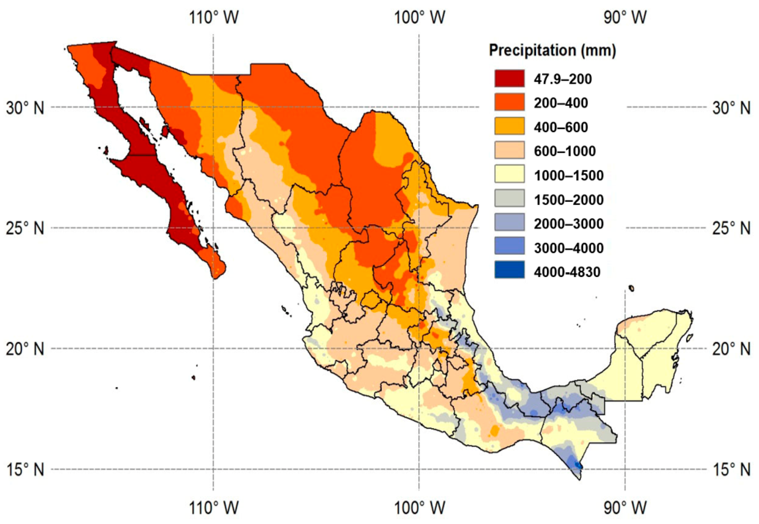
The spatial hydro-climatic gradients that motivate this classification are illustrated in Figure 2, which shows mean annual precipitation alongside the regional boundaries in Figure 1. Rainfall in Mexico spans more than an order of magnitude: from below 300–400 mm yr−1 in Baja California, Sonora, and Mapimí to above 2000 mm yr−1 in the Grijalva–Usumacinta and Papaloapan basins of the southeast [13,14]. Temperature and evaporative demand follow an inverse pattern—northern and interior basins experience high potential evapotranspiration and strong summer drought stress, while humid tropical basins sustain high rainfall and perennial baseflow even through the dry season. As a result, streamflow regimes differ sharply across regions. In the northwest and interior plateau, many rivers are intermittent or strongly regulated; dry-season discharges can approach zero for weeks, and observed 7-day minimum averages (7Q) at individual stations often fall below 0.1–0.5 m3 s−1. In contrast, tropical rivers in southern and Gulf-slope basins (e.g., Papaloapan, Grijalva–Usumacinta) are perennial; even during the low-flow season, 7Q values commonly remain one to two orders of magnitude higher than in arid basins. Transitional systems in central Mexico (e.g., Lerma–Santiago, Balsas) show mixed behavior: groundwater sustains some baseflow, but chronic over-extraction and reservoir operation can impose prolonged artificial low-flow periods during the dry season. These contrasts underline a key statistical challenge: no single unimodal probability distribution is likely to capture both (i) near-zero, drought-driven intermittence in semi-arid rivers and (ii) persistently positive perennial baseflows in humid tropical systems. This motivates testing flexible mixture distributions for national-scale low-flow frequency analysis.
As shown in Figure 1 and Figure 2, the 37 RHS of Mexico encompass a wide range of climatic and physiographic settings, from the arid basins of Baja California and the northern plateau to the humid tropical systems of the southeast. This spatial diversity justifies the regional grouping adopted in this study, whereby RHS were classified into (i) northern and northwestern arid regions, (ii) central highlands and transition zones, (iii) Gulf of Mexico basins, and (iv) southern tropical basins. Such grouping facilitates the interpretation of low-flow dynamics in relation to climate gradients, water use pressures, and management challenges across the country. Importantly, these sharp hydro-climatic contrasts highlight the limitations of single univariate models and motivate the use of Mixture Probability Distributions, which can better capture the diverse low-flow regimes observed across Mexico.
  • Northern and Northwestern Arid Regions (RHS 1–11, 34–35, 37)
This set of regions covers much of Baja California, Sonora, and the inland arid basins of northern Mexico, including Baja California Noroeste (RHS 1), Baja California Suroeste (RHS 3), Sonora Norte (RHS 8), Sonora Sur (RHS 9), Sinaloa (RHS 10), Presidio–San Pedro (RHS 11), Cuencas Cerradas del Norte (RHS 34), Mapimí (RHS 35), and El Salado (RHS 37). These areas are characterized by arid and semi-arid climates, with annual precipitation often below 400 mm and strong seasonality. Rivers are intermittent or highly regulated, and low flows are largely controlled by groundwater recession and reservoir operation. Droughts are recurrent, and evapotranspiration rates are among the highest in the country.
  • Central Highlands and Transition Zones (RHS 12–20, 36)
This zone includes Lerma–Santiago (RHS 12), Río Huicicila (RHS 13), Río Ameca (RHS 14), Costa de Jalisco (RHS 15), Armería–Coahuayana (RHS 16), Costa de Michoacán (RHS 17), Balsas (RHS 18), Costa Grande de Guerrero (RHS 19), Costa Chica de Guerrero (RHS 20), and Nazas–Aguanaval (RHS 36). These regions correspond to temperate to semi-humid climates, with rainfall ranging from 700 to 1200 mm per year. The Lerma–Santiago basin (RHS 12) is heavily populated and industrialized, and together with the Balsas basin (RHS 18) represents one of the most water-stressed parts of the country due to aquifer overexploitation and high demand.
  • Gulf of Mexico Basins (RHS 21–29)
The Gulf slope includes Costa de Oaxaca (RHS 21), Tehuantepec (RHS 22), Costa de Chiapas (RHS 23), Bravo–Conchos (RHS 24), San Fernando–Soto La Marina (RHS 25), Panuco (RHS 26), Norte de Veracruz (RHS 27), Papaloapan (RHS 28), and Coatzacoalcos (RHS 29). These regions are generally humid subtropical to tropical, with annual rainfall often exceeding 1500 mm. Rivers are perennial but exhibit sharp seasonal contrasts. They are important for hydropower, irrigation, and ecosystems, but low-flow droughts can still stress ecological flows and agricultural activities.
  • Southern Tropical Basins (RHS 30–33)
This group includes the Grijalva–Usumacinta (RHS 30) and the three Yucatán regions (RHS 31–33). The Grijalva–Usumacinta system sustains some of the largest discharges in Mexico, with annual rainfall frequently above 2000 mm. By contrast, the Yucatán basins are karstic, with few surface rivers but extensive groundwater networks, making low-flow processes distinct and tied to aquifer dynamics.
  • Hydro-Climatic Relevance
This spatial diversity across 37 RHS explains why no single univariate distribution can adequately represent low-flow regimes at the national scale. Arid northern basins require flexible models to capture intermittent and drought-dominated patterns, while humid southern basins demand approaches that represent persistent perennial baseflows. Mixture Probability Distributions provide a natural solution to capture this variability, consistent with Mexico’s regionalized water management framework.

2.2. Data Set

Daily streamflow records from 293 gauging stations with at least 20 years of data were obtained from the national hydrological network [15], (Table 1). For each station, annual minima of 7-day averages (7Q series) were extracted following established low-flow methods [1,2].

Record Length and Data Quality

All stations included in the analysis satisfied two screening criteria: (i) at least 20 complete hydrological years of daily discharge data, and (ii) identifiable and internally consistent metadata regarding station location and gauge operation period. Although 30-year records are commonly recommended for low-flow frequency studies, particularly for regulatory design flows [1,2], enforcing a strict 30-year minimum would have excluded a substantial fraction of drought-prone basins in northern Mexico and several heavily managed central basins. We therefore adopted a ≥20-year threshold to preserve spatial representativeness across all 37 RHS. For each time series we computed annual minima of 7-day mean flows (7Q series) only for years with at least 90% daily completeness; years with gaps exceeding 10% of daily observations during the relevant low-flow season were discarded from the 7Q extraction. After screening, the retained records typically span from the late 1920s–1930s through the 2000s–2010s, depending on the station, with median effective record length above 37 years and missing-data fractions below 5% of days in the low-flow season. This filtering ensures that the low-flow samples used for frequency analysis are not dominated by short or fragmented records.

2.3. Probability Distributions for Low-Flow Frequency Analysis

To evaluate the statistical behavior of 7Q flows, both univariate and Mixture Probability Distributions were considered. The univariate case included four classical families—LN3, G3, G, and W3—whose probability density functions (PDFs) are defined by combinations of location, scale, and shape parameters. These models provide a straightforward framework for estimating low-flow quantiles, but they may lack flexibility when confronted with multimodal, highly skewed, or heterogeneous samples.
To address these limitations, two-component mixture distributions were also applied. A mixture model combines two distinct univariate distributions, each with its own parameter set, weighted by a mixing proportion “p” constrained between 0 and 1. Mathematically, the overall PDF is expressed as a convex combination of the component densities, enabling mixtures to capture complex low-flow regimes that cannot be adequately represented by a single distribution. This flexibility makes mixture models particularly suited for hydro-climatic contexts where diverse generating processes govern low-flow behavior.

2.3.1. Univariate Distributions

  • Lognormal 3-parameter distribution [3,5]
    f x ;   x 0 ,   μ y ,   σ y = 1 x x 0 σ y 2 π e x p 1 2 ln x x 0 μ y σ y 2               x > x o
    where x 0 is the location parameter, μ y is the scale parameter, and σ y is the shape parameter.
  • Gamma 3-parameter distribution [16,17]
    f x ; x 0 , α , β = 1 α   Γ ( β ) x x 0 α β 1 e x x 0 α                 x > x o
    where x 0 is the location parameter, α is the scale parameter, and β is the shape parameter.
  • Gumbel distribution [18,19]
    f x ; ν , α = 1 α e x p e x p ν x α e x p ν x α ,     < x <
    where υ   is the location parameter and α is the scale parameter.
  • Weibull 3-parameter distribution [20,21]
    f x ; γ , β , α = α β γ x γ β γ α 1 e x γ β γ α ,                 x [ γ , )
    where γ is the location parameter x > γ , β is the scale parameter β > 0 , and α is the shape parameter α > 0 .

2.3.2. Mixture Distributions

Annual minimum flows result from the progressive depletion of a basin’s water storage until discharge reaches its lowest level. In some rivers, this recession is primarily driven by evaporation, whereas in others it results from the combined effects of evaporation and the lack of rainfall-driven recharge [22]. When such distinct mechanisms produce events that belong to different subpopulations, their combined behavior can be represented by a model that accounts for both groups simultaneously. This approach is formalized through mixture distributions [12,23], also known as blended distributions [23]:
F x = p F 1 x + 1 p F 2 x
where F x is the cumulative distribution function (CDF) of the mixture, F 1 x and F 2 x are the component CDFs, and p is the mixing proportion that determines the relative contribution of each component.
  • Mixture G–G
               f x ; ν 1 , α 1 , ν 2 , α 2 , p = p 1 α 1 e x p e x p ν 1 x α 1 e x p ν 1 x α 1 + 1 p 1 α 2 e x p e x p ν 2 x α 2 e x p ν 2 x α 2
  • Mixture G–W3
                f x ; ν 1 , α 1 , γ 2 , β 2 , α 2 , p = p 1 α 1 e x p e x p ν 1 x α 1 e x p ν 1 x α 1 + 1 p α 2 β 2 γ 2 x γ 2 β 2 γ 2 α 2 1 e x γ 2 β 2 γ 2 α 2
  • Mixture W3–G
                    f x ; γ 1 , β 1 , α 1 , ν 2 , α 2 , p = p α 1 β 1 γ 1 x γ 1 β 1 γ 1 α 1 1 e x γ 1 β 1 γ 1 α 1 + 1 p 1 α 2 e x p e x p ν 2 x α 2 e x p ν 2 x α 2
  • Mixture W3–W3
                    f x ; γ 1 , β 1 , α 1 , γ 2 , β 2 , α 2 , p = p α 1 β 1 γ 1 x γ 1 β 1 γ 1 α 1 1 e x γ 1 β 1 γ 1 α 1 + 1 p α 2 β 2 γ 2 x γ 2 β 2 γ 2 α 2 1 e x γ 2 β 2 γ 2 α 2

2.4. Estimation of Parameters

The parameters of all univariate and mixture distributions were estimated using the maximum likelihood estimation (MLE) method, which provides asymptotically efficient and unbiased estimates under general conditions.
The likelihood function is defined as:
L x , θ = i = 1 n f x i , θ
and the corresponding log-likelihood function is:
l n L x , θ = i = 1 n l n f x i , θ
Maximum likelihood estimators (MLEs) for the parameters of both univariate and mixture distributions are obtained by maximizing Equation (11). Given the nonlinear nature of the optimization problem, Rosenbrock’s restricted multivariate nonlinear optimization algorithm is employed [24].

2.5. Goodness-of-Fit Tests and Decision Criterion

The adequacy of each candidate distribution is evaluated using two empirical distribution function (EDF) tests: the Kolmogorov–Smirnov (K–S) and Anderson–Darling (A–D) statistics [25,26,27,28,29,30,31,32]. Both compare the empirical cumulative distribution function (ECDF) of the sample with the fitted theoretical cumulative distribution function F x , but they weight deviations differently—a distinction that is particularly relevant in extreme-value applications, where tail behavior is critical.

2.5.1. Kolmogorov–Smirnov Test

Let F x be a continuous candidate CDF and x 1 x n with empirical distribution function:
F n x = 1 n i = 1 n I x i x
The K–S statistic is defined as the maximum vertical distance between F n x and F x :
D n = F n x F x x s u p
The null hypothesis H0 states that the data are an i.i.d. sample from F x . Large values of D n indicate poor agreement between the ECDF and the fitted CDF. Critical values and p-values are obtained from the (asymptotic) sampling distribution of D n under H0, with appropriate adjustments when parameters are estimated from the data. The K–S test is a global goodness-of-fit (GOF) measure and is most sensitive near the center of the distribution, with comparatively less sensitivity in the tails—an important limitation in hydrological and extreme-value analyses.

2.5.2. Anderson–Darling Test

The Anderson–Darling test refines EDF-based GOF assessment by assigning greater weight to discrepancies in the distribution tails. For a continuous CDF F x and ordered sample x 1 x n , define
z i = F x i ,   i = 1 , 2 , , n
The A–D statistic is
A 2 = n 1 n i 1 n 2 i 1 l n z i + l n 1 z n + 1 i
Under H0, the data are i.i.d. from F x , and large values of A 2 indicate poor agreement between the sample and the fitted distribution. For many distributions, the A–D test has higher power than the K–S test to detect subtle but important deviations, especially in the tails, which is crucial for modeling extreme rainfall, floods, droughts, and wind speeds.

2.5.3. Integrated Decision Criterion for Model Selection

K–S and A–D tests are applied to each candidate distribution (e.g., LN3, G3, G, W3, G–G, G–W3, W3–G, W3–W3) using the fitted CDFs with parameters estimated from the sample. Goodness-of-fit results are combined through the following hierarchical decision rule:
(a)
At significance level α = 0.05, a model is considered acceptable if its p-value > α.
(b)
Among acceptable models, preference is given to those with smaller A 2 and larger p-values (especially from the A–D test).
(c)
Because of its emphasis on tail discrepancies, the A–D test is taken as the primary GOF indicator for extreme-value applications and design return levels.
(d)
If competing models exhibit similar A–D performance, the model with the smaller K–S statistic D n is preferred, reflecting better overall agreement with the ECDF.
(e)
If all models are rejected by at least one test, or if GOF statistics are very similar, the final choice is based on likelihood-based criteria (AIC, BIC [33,34]; lower values indicating a better balance between fit and parsimony) together with graphical diagnostics (P–P and Q–Q plots). In such cases, the selected distribution is explicitly reported as the least inadequate rather than formally adequate.
(f)
If the K–S test is accepted but the A–D test is rejected, this typically indicates an adequate global shape but poor tail representation; such models are treated with caution or discarded for extreme-quantile estimation.
(g)
If the A–D test is accepted and the K–S result is borderline, and likelihood-based criteria and tail-focused plots are satisfactory, the model may still be accepted for engineering purposes, prioritizing correct tail behavior.
This combined framework exploits the complementary strengths of the K–S and A–D tests and aligns the selection criterion with the primary objective of reliable estimation of extreme quantiles.
2.6. Bootstrap Procedure for Uncertainty Quantification

Sampling uncertainty in fitted parameters and design quantiles is assessed using a nonparametric bootstrap [35,36]. For each station and selected model, 1000 resamples of size n are drawn with replacement from the original series, parameters are re-estimated for each resample, and the corresponding T-year return levels are computed. The empirical distribution of these bootstrap return levels provides a direct estimate of variability and skewness. Two-sided 95% confidence intervals are obtained using the percentile method, i.e., from the 2.5% and 97.5% empirical quantiles. These intervals, which are often asymmetric for high return periods, quantify the reliability of the estimated extremes and complement the goodness-of-fit and information-criterion-based model selection.

3. Results

3.1. Quality Control Analysis

For each station, the 7Q series was subjected to a comprehensive quality-control procedure, including outlier detection (Grubbs), independence verification (Anderson), homogeneity assessment (Pettitt, Standard Normal, Buishand, and Von Neumann), and trend analysis (Mann–Kendall). Table 2 summarizes the outcomes of this quality assessment for station 30016.
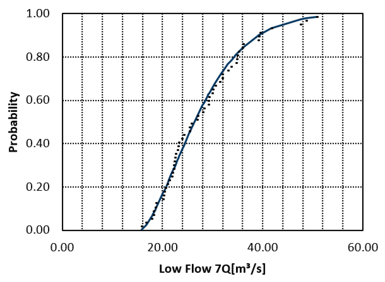
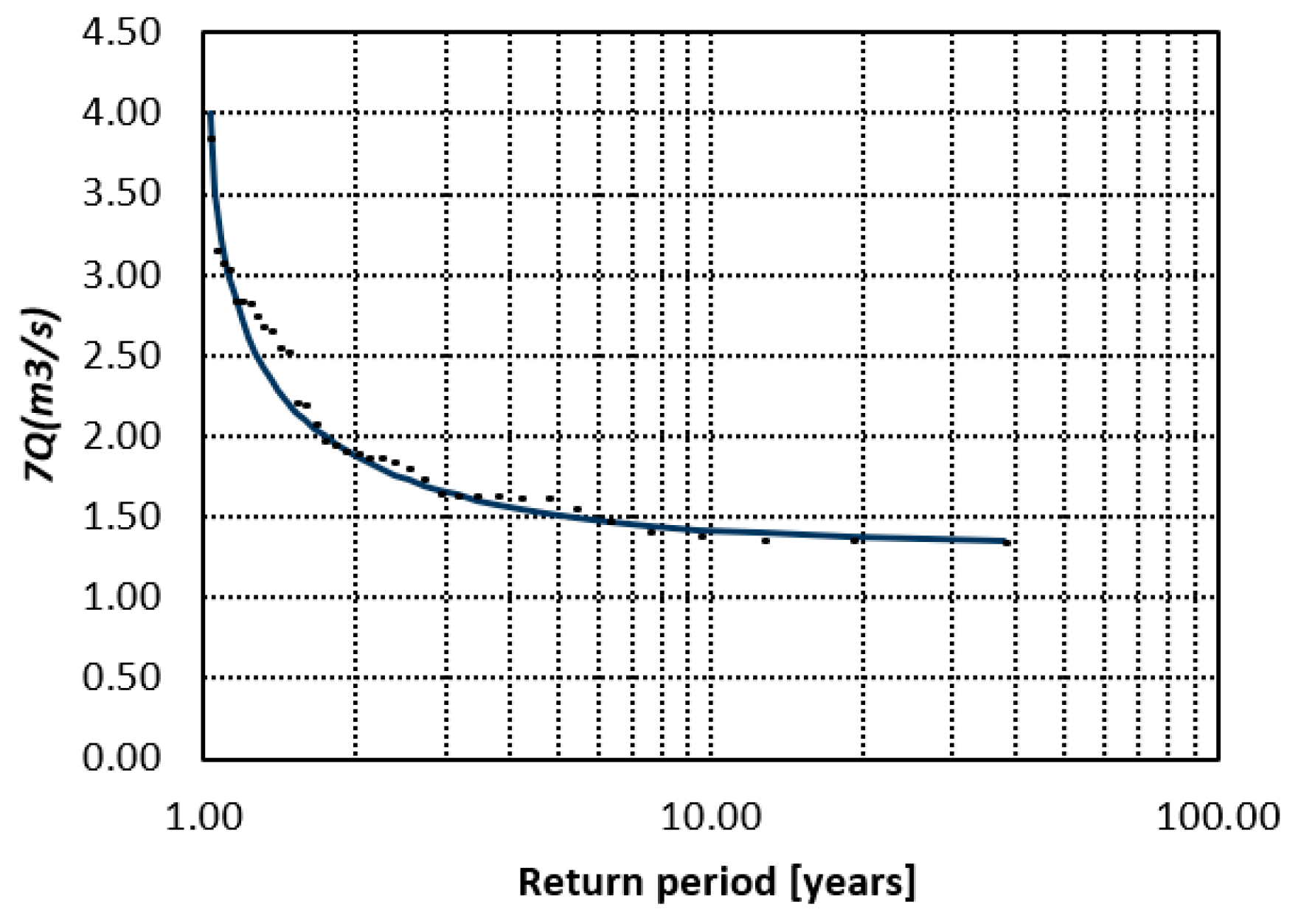
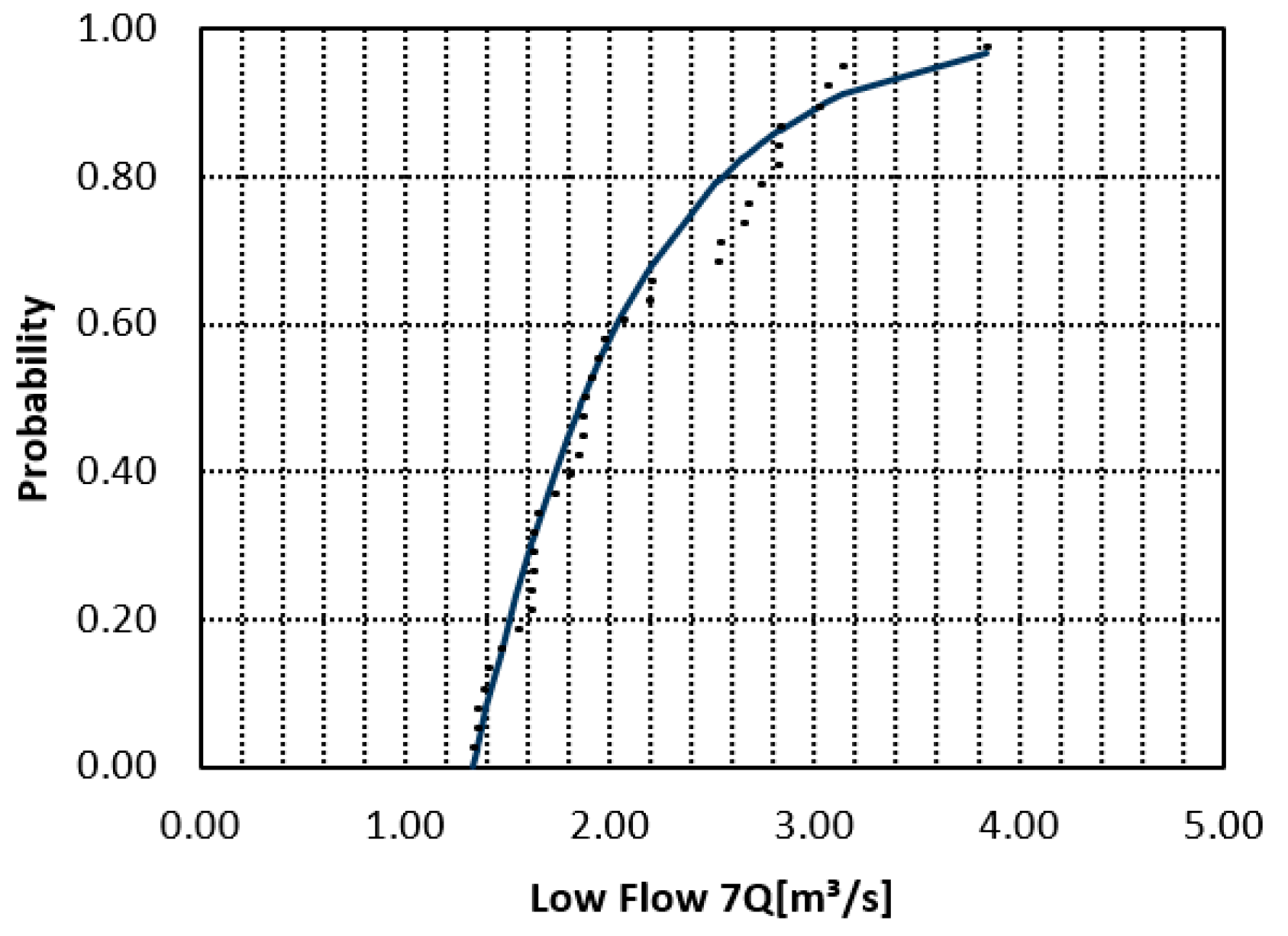
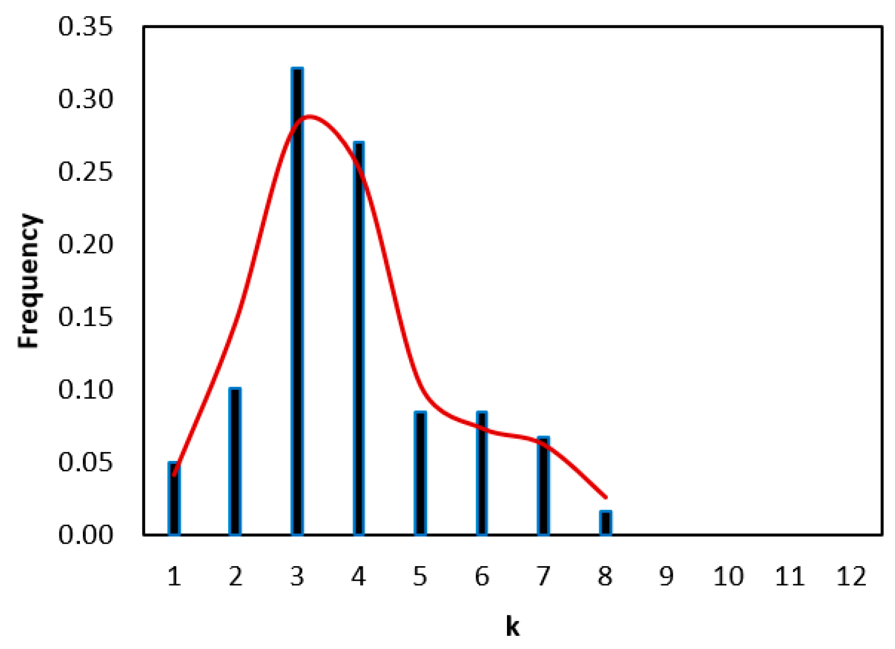
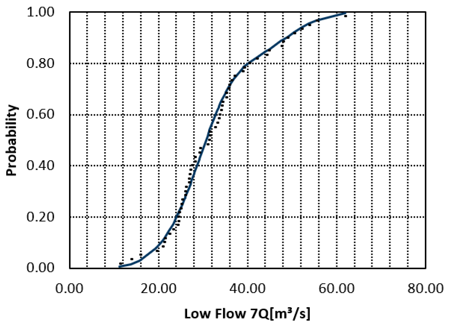
Low-flow frequency analysis was conducted for 293 gauging stations across the study area, using both univariate distributions (LN3, G3, G, and W3) and mixture models (G–G, G–W3, W3–G, W3–W3). Among the mixtures tested, the G–W3 and W3–W3 combinations consistently provided the best fit in a majority of stations, particularly in reproducing the central tendency and tail behavior of the distributions. To illustrate the procedure and the advantages of the mixture approaches, Table 3 and Figure 3, Figure 4 and Figure 5present the results for station 30016 (Region 30) as a representative example. The histogram of class marks (Figure 3) shows that the Weibull-3–Weibull-3 mixture captures the empirical frequency distribution more accurately than univariate alternatives. The return period plot (Figure 4) highlights the ability of the mixture distribution to match empirical quantiles across a wide range of recurrence intervals, while the probability plot (Figure 5) confirms the adequacy of the mixture model in reproducing the cumulative distribution of observed low flows. Overall, the results from station 30016 illustrate the improved performance of mixture distributions compared to traditional univariate approaches, a finding that is consistent across many of the 293 stations analyzed.

3.2. National Overview

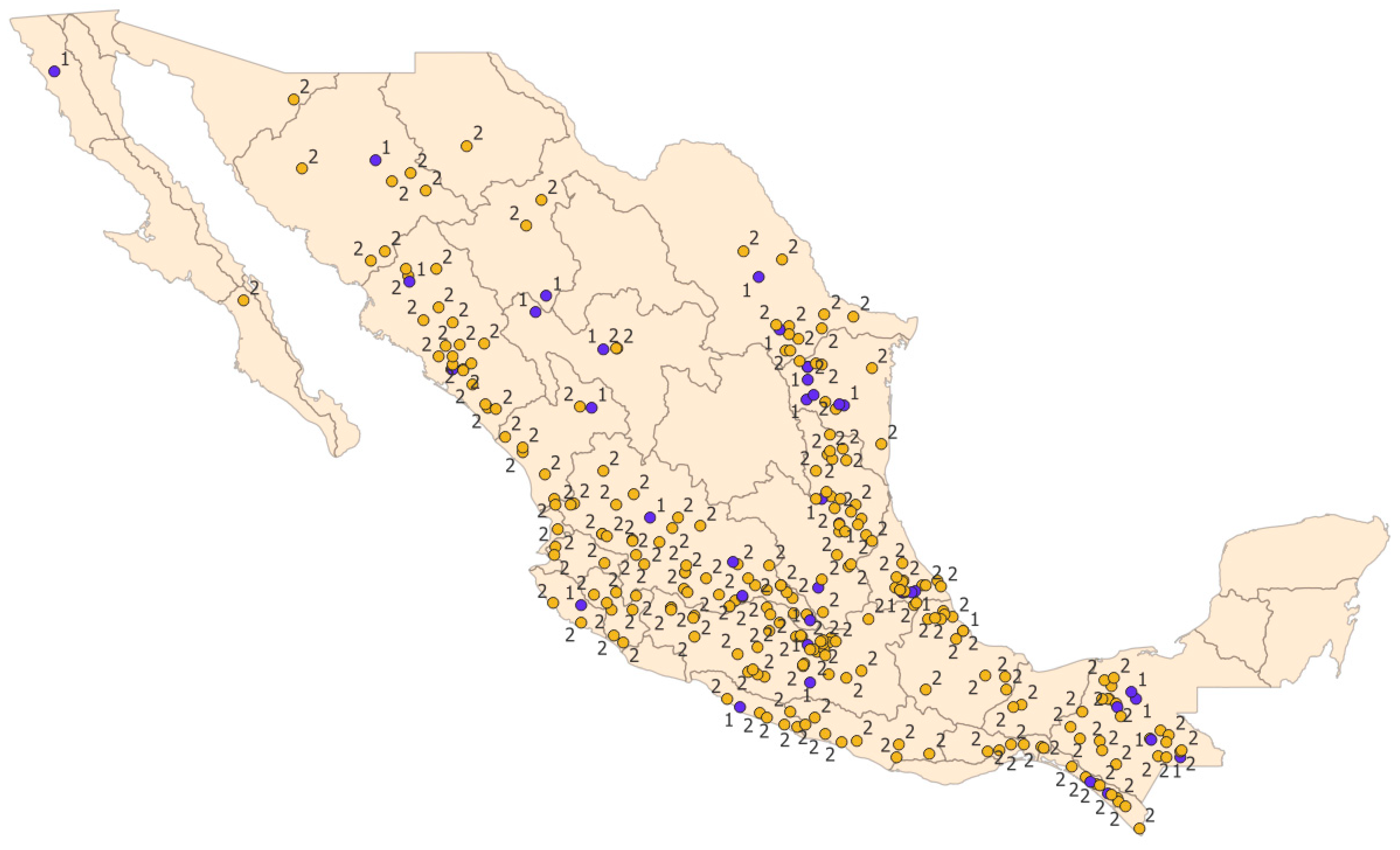
While the results at station 30016 illustrate the advantages of mixture distributions in representing low-flow frequency behavior, extending the analysis to 293 gauging stations confirms this tendency at a national scale. Figure 6 maps station locations and codes the best-fitting model class (univariate vs. mixture), making spatial representativeness and regional clustering explicit.
Table 4 summarizes the best-fitting models by hydrological region. According to the K–S and A–D tests, complemented by information criteria, only 40 out of 293 stations (13.7%) are best represented by univariate distributions, whereas 253 stations (86.3%) are better fitted by mixture models. Among the univariates, LN3 dominates (32 stations), followed by W3 (5) and G3 (3), while the Gumbel distribution is never selected as the optimal model.
Mixture distributions clearly prevail at the national scale. The W3–W3 mixture is the single most frequent best-fitting model (132 stations; 45.1% of all sites; 52.2% of mixture cases), followed by G–W3 (65 stations; 22.2% of all; 25.7% of mixtures) and W3–G (54 stations; 18.4% of all; 21.3% of mixtures). The symmetric G–G mixture is selected only at two stations (<1%). These results confirm the flexibility of Weibull-based mixtures to capture diverse low-flow regimes and complex distributional shapes that cannot be adequately modeled by classical univariate distributions alone.
To complement the single-station example (station 30016), additional diagnostic plots analogous to Figure 3, Figure 4 and Figure 5 are provided in Appendix A (Figure A1, Figure A2, Figure A3, Figure A4, Figure A5 and Figure A6).

3.3. Regional Patterns

The dominance of mixture models is also evident at the regional scale. In most RHS, mixtures account for ≥80% of best fits, and in several regions (e.g., 3, 13, 14, 16, 20, 22, 29, 34) they represent 100% of the selected models. Univariate distributions prevail only in region 1 (single station) and share dominance with mixtures in region 36, while in the remaining regions their contribution is minor. This consistent pattern indicates that low-flow processes across Mexico often reflect the superposition of distinct hydrological regimes (e.g., baseflow-dominated vs. drought-driven conditions), which are more realistically represented by mixture distributions.
These spatial results, in combination with the single-station diagnostics (Figure 3, Figure 4 and Figure 5), support the robustness and coherence of mixture-based low-flow frequency modeling under contrasting hydro-climatic settings, from arid and semiarid basins to humid tropical and temperate catchments.

3.4. Return Levels and Uncertainty Bounds

To further assess the performance of the fitted models, return levels of 7Q were computed for a set of representative stations and a range of design return periods. These examples allow direct comparison between univariate distributions and mixture models under contrasting hydro-climatic conditions and complement the national and regional analyses. Appendix B summarizes, for selected stations, the estimated return levels and their associated uncertainty (Table A1, Table A2, Table A3, Table A4, Table A5 and Table A6).
Uncertainty was quantified explicitly by constructing 95% confidence intervals (CIs) for each return level using the nonparametric bootstrap procedure described in Section 2.6. For each station–model combination, the 7Q series was resampled with replacement, parameters were re-estimated for each bootstrap sample, and empirical percentiles of the resulting return levels were used to derive lower and upper CIs. The tables in Appendix B report, for each return period T, the point estimate, the 95% CI limits, and the CI range. Across stations, mixture models—particularly W3–W3 and G–W3—systematically yield narrower CIs than the best univariate competitors (most often LN3), indicating reduced sampling uncertainty and more stable extrapolation of extreme low flows.
As an illustration, Table 5 presents 7Q return levels and 95% confidence intervals for station 30016, comparing the best univariate model (LN3) with the W3–W3 mixture. The mixture exhibits systematically narrower intervals, confirming its improved precision for extreme low-flow estimation.
The Gumbel distribution and the symmetric G–G mixture produced negative return levels at higher return periods for several stations, due to the interaction between location and scale parameters in the Gumbel quantile function. As river flows are non-negative, these extrapolations are physically implausible, making Gumbel-only models the least reliable option for rare-event low-flow estimates, even when their formal GOF statistics are acceptable.
When Gumbel is combined with Weibull-3 (G–W3 and W3–G), this problem is mitigated. The Weibull-3 component, with lower-bounded support [γ, ∞), constrains the lower tail and prevents negative extrapolations. In practice, maximum likelihood estimation tends to assign greater weight to the Weibull–3 in the tail, ensuring hydrologically realistic, non-negative return levels while preserving flexibility in the body of the distribution. As a result, W3–W3 and G–W3 mixtures emerge as the most robust choices, combining good fit, physically consistent support, and comparatively narrow CIs.
Overall, the joint analysis of point estimates and bootstrap CIs highlights three key aspects: (i) sampling variability can be substantial at long return periods and must be made explicit; (ii) structural uncertainty is reduced when mixtures are considered alongside classical univariate models; and (iii) distributions with bounded support and mixture formulations provide more reliable and defensible design flows. Reporting CIs, as done here, allows agencies to assess whether differences between basins or models are statistically meaningful when prioritizing drought-management and low-flow mitigation measures.
The importance of incorporating confidence intervals into model selection is clearly illustrated at station 25034 (Region 25). Although the A–D and K–S statistics for the W3 and W3–G distributions are nearly identical (Table A5), the bootstrap-based 7Q return levels (Table A6) show that the W3 model systematically yields narrower and more stable 95% confidence intervals than W3–G. This contrast demonstrates that, when goodness-of-fit statistics alone are inconclusive, uncertainty bounds provide essential additional discrimination and may justify selecting one model over another, even if their EDF-based metrics appear similar.

4. Discussion

The national results confirm that two-component mixture models provide a more reliable and flexible framework for low-flow frequency analysis in hydro-climatically diverse settings. Based on the integrated goodness-of-fit and information-criteria procedure, mixture distributions are selected as the best-fitting models at 86.3% of the 293 stations, with a clear dominance of Weibull-based mixtures. The W3–W3 mixture alone accounts for 45.1% of all stations (52.2% of mixture cases), followed by G–W3 and W3–G, while Gumbel-only models are never preferred. The single-station diagnostics for 30016, together with the regional summary in Table 3, show that mixtures improve both central fit and tail behavior and yield narrower bootstrap confidence intervals for design return levels than the best-performing univariate alternatives (typically LN3).
These findings are consistent with the conceptual understanding that low flows often arise from more than one generating mechanism. In many Mexican basins, annual minimum flows reflect the interplay between groundwater-fed baseflow, regulated releases, and drought-induced depletion. A single unimodal distribution cannot easily accommodate such structural heterogeneity, whereas finite mixtures can represent distinct regimes via their component distributions and mixing weights. In this sense, the success of W3–W3 and G–W3 is not purely numerical: it reflects their ability to encode lower-bounded, hydrologically consistent behavior while retaining flexibility in skewness and kurtosis.
The explicit computation of bootstrap confidence intervals further strengthens these conclusions. For representative sites (e.g., station 30016), mixture models not only match the empirical distribution more closely but also exhibit systematically narrower 95% confidence intervals for 7Q return levels compared with LN3. This indicates reduced sampling variability and more stable extrapolation for regulatory design flows. Conversely, Gumbel-only and G–G mixtures generate negative return levels at long return periods in several cases; such outcomes are physically implausible for discharge and highlight the risk of relying on unbounded left-tail models for low-flow design.

4.1. Implications for Management

4.1.1. Relevance for Environmental Impact Assessment

Environmental Impact Assessments (EIA) in Mexico and internationally often require reliable estimates of design low flows, particularly the 7Q10 statistic, which represents the minimum 7-day average flow expected once every ten years. This metric is fundamental for evaluating effluent dilution capacity, setting ecological flow thresholds, and ensuring compliance with water quality standards.
However, traditional reliance on univariate probability models has often resulted in under- or overestimation, leading either to overly restrictive discharge limits or to insufficient protection of aquatic ecosystems.
The results of this study demonstrate that mixture distributions—especially the W3–W3 and G–W3 families—offer a superior representation of low-flow regimes across diverse hydro-climatic settings. By reducing bias in critical quantiles such as 7Q10, mixture models strengthen the scientific foundation of EIA procedures. This ensures that regulatory decisions are both environmentally protective and technically feasible for water users.
In arid basins of northern Mexico, underestimation of 7Q10 by univariate models can result in effluent permits that exceed the river’s real dilution capacity, increasing risks of water quality degradation. Conversely, in tropical basins, overestimation of 7Q10 may impose unnecessarily strict discharge limits, creating economic burdens without proportional environmental benefits. By providing more accurate and balanced estimates, mixture models reduce these risks and promote realistic, evidence-based standards.
Furthermore, because EIAs are often conducted at the basin or regional scale, the flexibility of mixture models aligns well with Mexico’s 37 RHS, allowing region-specific characterization of low flows that can be directly integrated into regulatory frameworks. Adopting mixture models in EIA protocols would therefore improve the robustness of environmental regulation, reduce uncertainty in effluent permitting, and enhance the credibility of water management decisions under increasing climatic variability.

4.1.2. Drought Management

For drought management, reliable low-flow quantiles underpin allocation rules, reservoir release policies, emergency triggers, and environmental flow safeguards. In semi-arid and drought-prone regions, mixture models capture severe low-flow states more realistically, while bootstrap CIs explicitly quantify the uncertainty associated with rare events. This combination supports risk-informed planning: agencies can (i) identify basins where 7Q10 (or other design quantiles) are estimated with high confidence, and (ii) recognize where wide intervals indicate the need for conservative margins, enhanced monitoring, or adaptive operation.

4.1.3. Regional Water Policy (CONAGUA Framework)

Mexico’s water planning is structured around 37 RHS [13,14]. Mixture models provide a natural fit for region-specific low-flow characterization, aligning statistical tools with CONAGUA’s institutional framework. Their adoption would allow more accurate and context-sensitive decisions, strengthening the integration of hydrological science with management practice.
Implementing mixture models in routine agency workflows does present practical challenges. Mixture fitting requires nonlinear optimization, which is more technically demanding than fitting a single-parameter family by moments or L-moments. Personnel may also need training to interpret multi-parameter models and to report design flows together with confidence bounds. However, these challenges are largely logistical rather than conceptual: the estimation procedures can be scripted in standard statistical software, and the outputs—design 7Q10 flows with documented uncertainty—map directly onto existing regulatory tasks such as effluent permitting, ecological flow setting, and drought contingency planning. In that sense, adopting mixtures does not require redefining policy instruments; it requires upgrading the statistical tools used to populate those instruments.
An important practical insight emerges when goodness-of-fit statistics alone are inconclusive. At station 25034 (Region 25), the W3 and W3–G models exhibit almost identical A–D and K–S values (Table A5), which under a purely EDF-based criterion would suggest statistical equivalence. However, the bootstrap results (Table A6) show that the W3 distribution systematically yields narrower and more stable 95% confidence intervals for 7Q return levels than the W3–G mixture. This example illustrates that uncertainty bounds are not merely supplementary diagnostics but a decisive element of model selection: when fits are similar, the model providing physically consistent estimates with tighter and more regular confidence intervals should be preferred. In this sense, the proposed framework does not automatically favor mixtures; instead, it combines EDF tests, information criteria, and bootstrap-based uncertainty to identify the least inadequate and most reliable model for operational use.

4.2. Limitations of the Study

Despite the robust performance of mixtures, several limitations must be acknowledged.
First, all analyses are conducted under the assumption of statistical stationarity of the 7Q series. Although homogeneity and trend tests (e.g., Pettitt, Buishand, Von Neumann, Mann–Kendall) were applied and series showing strong inconsistencies were screened, this does not preclude gradual non-stationary changes driven by climate variability, groundwater depletion, land-use change, or regulation. In basins where low flows are deteriorating, stationary return levels may underestimate emerging risks.
Second, the minimum record length criterion (≥20 years) represents a compromise between statistical robustness and spatial coverage. This choice preserves representation in drought-prone and managed basins but limits the precision of long return-period estimates at some sites, as reflected in wider confidence intervals for high T, even under mixture models.
Third, mixture models require nonlinear optimization and careful numerical implementation. Although maximum likelihood estimation was successfully applied here, convergence issues or local optima may arise in shorter or noisier records. These aspects must be handled carefully in operational settings through diagnostics and robust algorithms.
Finally, the analysis focuses on univariate 7Q-based indicators. Other dimensions of hydrological drought—such as deficit volume, duration, and timing—are not explicitly modeled, even though they are relevant for ecological impacts and reservoir operation.

4.3. Future Work

Three extensions are especially relevant. First, non-stationary formulations of mixture models should be developed so that parameters (e.g., scale or location) evolve with time, climate indices (ENSO/PDO), groundwater levels, or indicators of human pressure such as reservoir storage and abstraction intensity. This would allow direct quantification of how drought severity is changing rather than assuming a constant regime. Second, although this study focused on two-component parametric mixtures for transparency and ease of adoption by regulatory agencies, alternative frameworks such as semi-parametric kernel methods, quantile regression, or machine-learning models could be explored to capture highly non-monotonic behavior without prescribing a specific functional form. Third, extending beyond univariate low-flow characterization toward bivariate or multivariate structures (e.g., via copula-based methods) would allow joint assessment of drought duration, deficit volume, and timing, which are essential for ecological impact and reservoir operation. Together, these extensions would move Mexican low-flow regulation from a stationary, one-metric paradigm toward a dynamic, risk-based framework.

5. Conclusions

Using 7-day annual minimum flows (7Q series) from 293 gauging stations across Mexico’s 37 RHS, this study evaluated both traditional univariate probability distributions and flexible two-component mixture models. Nationally, mixture distributions outperformed single-family models in the large majority (86.3%) of the stations analyzed. The W3–W3 and G–W3 mixtures were the most frequently selected best-fit models, particularly in arid and tropical regions where low-flow regimes are shaped by distinct physical processes such as groundwater recession, reservoir operation, and pronounced dry seasons.
These results have direct management implications. For Environmental Impact Assessment, more reliable estimates of the 7Q10 design flow reduce regulatory uncertainty when setting effluent dilution requirements and ecological flow thresholds. For drought management, mixture-based quantiles improve the robustness of allocation rules, reservoir operation targets, and emergency triggers in water-scarce basins. For regional water policy, the strong performance of mixtures across CONAGUA’s hydrological planning regions indicates that these models can be integrated into basin-scale decision-making in a way that reflects actual hydro-climatic diversity rather than assuming a single nationwide “typical” regime.
Beyond the performance gains, this work highlights that univariate models can produce physically implausible return levels (e.g., negative flows at long return periods), whereas mixtures that include lower-bounded components avoid this issue and therefore yield more defensible design values. We also identify two priorities for future application: incorporating explicit uncertainty bounds (e.g., confidence intervals for design flows) and extending the framework to non-stationary conditions driven by climate variability, groundwater depletion, and changing water demand.
Cases such as station 25034 demonstrate that comparable A–D and K–S statistics for different models (e.g., W3 vs. W3–G) can mask meaningful differences in the width and stability of bootstrap confidence intervals. Incorporating uncertainty bounds into the selection framework favors models that are both statistically adequate and more precise, and in some instances justifies choosing a parsimonious univariate model over a more complex mixture. This reinforces the recommendation that design 7Q10 values and regulatory decisions should be based on joint evaluation of fit, physical plausibility, and quantified uncertainty, rather than on GOF statistics alone.
In summary, Mixture Probability Distributions are not only statistically superior in many Mexican basins, but they are operationally relevant. Incorporating them—especially the W3–W3 and G–W3 families—into national low-flow guidelines would improve the technical basis for environmental regulation, drought preparedness, and regional allocation policy under increasing hydro-climatic stress.

Funding

This research received no external funding.

Data Availability Statement

The original data presented in the study are openly available in CONAGUA’s National Hydrometric Network at https://sih.conagua.gob.mx/hidros.html, accessed on 1 March 2025.

Conflicts of Interest

The author declares no conflicts of interest.

Abbreviations

The following abbreviations are used in this manuscript:
7Q7-day minimum average flow
7Q107Q associated with a 10-year return period
RHSHydrological Planning Regions of Mexico
CONAGUANational Water Commission

Appendix A. Station Locations and Example Diagnostics

This appendix complements the station-location map in Figure 6 by showing representative station-level diagnostics for three contrasting sites. Each station includes two plots: (i) return-level (quantile) plot, and (ii) probability (CDF) plot. Together, these illustrate how the selected model reproduces both the central body and the lower tail of the 7Q distribution.

Appendix A.1. Station 10063—Gumbel–Weibull-3 (G–W3) Mixture Best Fit

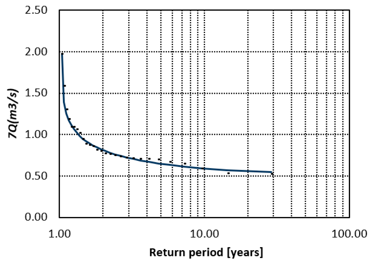
Figure A1. Return-level plot for 7Q at station 10063 (Region 10). Empirical quantiles (points) versus G–W3 fit (line) show close agreement across recurrence intervals.
Environments 12 00450 g0a1
Figure A2. Probability (CDF) plot for 7Q at station 10063 (Region 10). Observed non-exceedance probabilities (points) are well reproduced by the G–W3 fit (line).
Environments 12 00450 g0a2

Appendix A.2. Station 18439—Weibull-3 (W3) Best Fit

Figure A3. Return-level plot for 7Q at station 18439 (Region 18). Empirical quantiles (points) versus W3 distribution (line) highlight improved agreement at longer return periods.
Environments 12 00450 g0a3
Figure A4. Probability (CDF) plot for 7Q at station 18439 (Region 18). The W3 distribution (line) closely tracks observed non-exceedance probabilities (points), especially in the critical low-flow range.
Environments 12 00450 g0a4

Appendix A.3. Station 25034—Weibull-3 (W3) Best Fit

Figure A5. Return-level plot for 7Q at station 25034 (Region 25). Empirical quantiles (points) versus W3 distribution (line) highlight improved agreement at longer return periods.
Environments 12 00450 g0a5
Figure A6. Probability (CDF) plot for 7Q at station 25034 (Region 25). The W3 distribution (line) closely tracks observed non-exceedance probabilities (points).
Environments 12 00450 g0a6

Appendix B. Return-Level Estimates and Model Comparison

This appendix complements Section 3.4 by presenting return-level estimates of the 7-day annual minimum flow (7Q) for the same stations shown in Appendix A. For each station, we report the best-fitting univariate and mixture distributions together with their A–D and K–S statistics, followed by return levels (m3 s−1) and corresponding 95% confidence intervals for recurrence intervals from 2 to 100 years.

Appendix B.1. Station 10063—Gumbel–Weibull-3 (G–W3) Mixture Best Fit

Table A1. Anderson–Darling (A–D) and Kolmogorov–Smirnov (K–S) goodness-of-fit statistics for candidate distributions at station 10063 (Region 10); lower values indicate better agreement, with the G–W3 mixture providing the best overall fit. Results for G and G–G distributions are not included because they produced negative return levels, which are physically inconsistent for low flows.
Distribution
StatisticLN3G3W3G–W3W3–GW3–W3
A–D0.2740.4130.5020.2120.5020.361
K–S0.1020.1260.1370.0880.1370.114
Table A2. Estimated 7Q return levels for different return periods (T) at station 10063 (Region 10), including 95% confidence intervals (ICL–ICU) and their range (ICU–ICL). The G–W3 mixture model yields systematically narrower confidence intervals than the best univariate model (LN3), indicating reduced uncertainty in extreme low-flow estimates.
LN3 DistributionG–W3 Distribution
T (Years)95%ICL7Q95%ICURange95%ICL7Q95%ICURange
20.7230.8120.9300.2070.7010.8120.9260.225
50.5960.6540.7290.1330.5630.6450.7270.164
100.5510.5980.6790.1280.5260.5900.6870.160
200.4820.5620.6640.1810.5240.5580.6630.139
500.4090.5300.6520.2430.5180.5350.6500.132
1000.3650.5130.6470.2820.4970.5250.6490.152

Appendix B.2. Station 18439—Weibull-3 (W3) Best Fit

Table A3. Anderson–Darling (A–D) and Kolmogorov–Smirnov (K–S) goodness-of-fit statistics for candidate distributions at station 18439 (Region 18); lower values indicate better agreement, with the W3 distribution providing the best overall fit. Results for the G distribution are not included because they produced negative return levels, which are physically inconsistent for low flows.
Distribution
StatisticLN3G3W3G–GG–W3W3–GW3–W3
A–D0.4340.2260.2071.0210.6190.2250.255
K–S0.1040.0660.0710.1260.0980.0800.075
Table A4. Estimated 7Q return levels for different return periods (T) at station 18439 (Region 18), including 95% confidence intervals (ICL–ICU) and their range (ICU–ICL). The W3 distribution model yields systematically narrower confidence intervals than the best mixture model (W3–G), indicating reduced uncertainty in extreme low-flow estimates.
W3 DistributionW3–G Distribution
T (Years)95%ICL7Q95%ICURange95%ICL7Q95%ICURange
224.34026.36928.2703.93024.37926.52028.5824.203
519.56320.70122.0822.51919.60820.84522.4452.838
1017.83718.69020.2992.46217.81718.80020.5842.766
2016.84117.49419.2992.45816.51117.57119.1432.633
5016.08116.58318.4742.39314.66016.61818.3933.732
10015.64516.18318.2272.58113.03216.20018.1515.120

Appendix B.3. Station 25034—Weibull-3 (W3) Best Fit

Table A5. Anderson–Darling (A–D) and Kolmogorov–Smirnov (K–S) goodness-of-fit statistics for candidate distributions at station 25034 (Region 25); lower values indicate better agreement, with the W3 distribution providing the best overall fit. Results for G and G–G distributions are not included because they produced negative return levels, which are physically inconsistent for low flows.
Distribution
StatisticLN3G3W3G–W3W3–GW3–W3
A–D0.8281.3180.5771.1100.5780.736
K–S0.1260.1850.1160.1550.1160.161
Table A6. Estimated 7Q return levels for different return periods (T) at station 25034 (Region 25), including 95% confidence intervals (ICL–ICU) and their range (ICU–ICL). The W3 distribution model yields systematically narrower confidence intervals than the best mixture model (W3–G), indicating reduced uncertainty in extreme low-flow estimates.
W3 DistributionW3–G Distribution
T (Years)95%ICL7Q95%ICURange95%ICL7Q95%ICURange
21.5661.8732.1370.5711.6241.8652.2380.615
51.3531.5111.7300.3771.3441.4481.6790.335
101.3341.4171.5630.2291.3291.3761.5610.232
201.3301.3721.4530.1241.3281.3481.4750.147
501.3291.3461.3920.0631.3031.3351.4040.101
1001.3281.3371.3670.0391.2601.3311.3620.102

References

  1. Smakhtin, V.U. Low flow hydrology: A review. J. Hydrol. 2001, 240, 147–186. [Google Scholar] [CrossRef]
  2. Tallaksen, L.; van Lanen, H. (Eds.) Hydrological Drought: Processes and Estimation Methods for Streamflow and Groundwater; Elsevier: Amsterdam, The Netherlands, 2004. [Google Scholar]
  3. Haan, C.T. Statistical Methods in Hydrology, 2nd ed.; Iowa State Press: Ames, IA, USA, 2002. [Google Scholar]
  4. Vogel, R.M.; Kroll, C.N. Regional geohydrologic-geomorphic relationships for the estimation of low-flow statistics. Water Resour. Res. 1992, 28, 2451–2458. [Google Scholar] [CrossRef]
  5. Stedinger, J.R.; Vogel, R.M.; Foufoula-Georgiou, E. Frequency analysis of extreme events. In Handbook of Hydrology; Maidment, D.R., Ed.; McGraw-Hill: Columbus, OH, USA, 1993; pp. 18.1–18.66. [Google Scholar]
  6. Laaha, G.; Blöschl, G. Seasonality indices for regionalizing low flows. Hydrol. Process. 2006, 20, 3851–3878. [Google Scholar] [CrossRef]
  7. Castellarin, A.; Vogel, R.; Brath, A. A stochastic index flow model of flow duration curves. Water Resour. Res. 2004, 40, W03104. [Google Scholar] [CrossRef]
  8. Hisdal, H.; Tallaksen, L.; Gustard, T.; Clausen, B.; Peters, E. Chapter 5—Hydrological drought characteristics. In Hydrological Drought: Processes and Estimation Methods for Streamflow and Groundwater; Tallaksen, L.M., van Lanen, H.A.J., Eds.; Elsevier: Amsterdam, The Netherlands, 2004; Volume 2004, pp. 139–198. [Google Scholar] [CrossRef]
  9. Riggs, H.C. Low-Flow Investigations; U.S. Geological Survey, Techniques of Water-Resources Investigations; US Government Printing Office: Washington, DC, USA, 1972; Book 4, Chapter B1. [Google Scholar]
  10. US EPA. Technical Support Document for Water Quality-Based Toxics Control; Office of Water, U.S. Environmental Protection Agency: Washington, DC, USA, 1991. [Google Scholar]
  11. Kottegoda, N.; Rosso, R. Statistics, Probability, and Reliability for Civil and Environmental Engineers; McGraw-Hill: Columbus, OH, USA, 1998. [Google Scholar]
  12. Yilmaz, A.; Singh, V. Frequency analysis of hydrologic extremes using mixture distributions. J. Hydrol. Eng. 2012, 17, 1177–1189. [Google Scholar]
  13. CONAGUA. Atlas del Agua en México 2018. Comisión Nacional del Agua, Secretaría de Medio Ambiente y Recursos Naturales, México. 2018. Available online: https://files.conagua.gob.mx/conagua/publicaciones/Publicaciones/AAM2018.pdf (accessed on 1 March 2025).
  14. IMTA. Estadísticas del Agua en México; Instituto Mexicano de Tecnología del Agua: Jiutepec, México, 2021. [Google Scholar]
  15. CONAGUA. Red Nacional Hidrométrica: Datos Históricos de Estaciones de aforo; Comisión Nacional del Agua, Secretaría de Medio Ambiente y Recursos Naturales: México, México, 2024; Available online: https://sih.conagua.gob.mx/hidros.html (accessed on 1 March 2025).
  16. Thom, H. A note on the gamma distribution. Mon. Weather Rev. 1958, 86, 117–122. [Google Scholar] [CrossRef]
  17. Hosking, J.; Wallis, J. Regional Frequency Analysis: An Approach Based on L-Moments, 1st ed.; Cambridge University Press: Cambridge, MA, USA, 1997; ISBN 978-0-521-43045-6. [Google Scholar]
  18. Coles, S. An Introduction to Statistical Modeling of Extreme Values; Springer: Berlin/Heidelberg, Germany, 2001. [Google Scholar]
  19. Katz, R.; Parlange, M.; Naveau, P. Statistics of extremes in hydrology. Adv. Water Res. 2002, 25, 1287–1304. [Google Scholar] [CrossRef]
  20. Johnson, N.; Kotz, S.; Balakrishnan, N. Continuous Univariate Distributions; Wiley: Hoboken, NJ, USA, 1995; Volume 2. [Google Scholar]
  21. Rao, A.; Hamed, K. Flood Frequency Analysis; CRC Press: Boca Raton, FL, USA, 2000. [Google Scholar]
  22. Waylen, P.; Woo, M. Annual low flows generated by mixed processes. Hydrol. Sci. J. 1987, 3, 371–383. [Google Scholar] [CrossRef]
  23. Mood, A.; Graybill, F.; Boes, D. Introduction to the Theory of Statistics; McGraw-Hill: Columbus, OH, USA, 1974. [Google Scholar]
  24. Kuester, J.L.; Mize, J.H. Optimization Techniques with FORTRAN; McGraw-Hill: New York, NY, USA; Düsseldorf, Germany, 1973; ISBN 978-0-07-035606-1. [Google Scholar]
  25. Kolmogorov, A.N. Sulla determinazione empirica di una legge di distribuzione. G. Dell’istituto Ital. Degli Attuari 1933, 4, 83–91. [Google Scholar]
  26. Smirnov, N. Table for estimating the goodness of fit of empirical distributions. Ann. Math. Stat. 1948, 19, 279–281. [Google Scholar] [CrossRef]
  27. Massey, F.J. The Kolmogorov-Smirnov test for goodness of fit. J. Am. Stat. Assoc. 1951, 46, 68–78. [Google Scholar] [CrossRef]
  28. Anderson, T.; Darling, D. Asymptotic theory of certain “goodness-of-fit” criteria based on stochastic processes. Ann. Math. Stat. 1952, 23, 193–212. [Google Scholar] [CrossRef]
  29. Anderson, T.; Darling, D. A test of goodness-of-fit. J. Am. Stat. Assoc. 1954, 49, 765–769. [Google Scholar] [CrossRef]
  30. Stephens, M.A. EDF statistics for goodness of fit and some comparisons. J. Am. Stat. Assoc. 1974, 69, 730–737. [Google Scholar] [CrossRef]
  31. Stephens, M.A. Goodness-of-fit for the extreme value distribution. Biometrika 1977, 64, 583–588. [Google Scholar] [CrossRef]
  32. D’Agostino, R.B.; Stephens, M.A. (Eds.) Goodness-of-Fit Techniques; Marcel Dekker: New York, NY, USA, 1986. [Google Scholar]
  33. Akaike, H. A new look at the statistical identification model. IEEE Trans. Autom. Control. 1974, 6, 716–723. [Google Scholar] [CrossRef]
  34. Schwarz, G. Estimating the dimension of a model. Ann. Stat. 1978, 6, 461–464. [Google Scholar] [CrossRef]
  35. Efron, B.; Tibshirani, R.J. An Introduction to the Bootstrap; Chapman & Hall/CRC: Boca Raton, FL, USA, 1993. [Google Scholar]
  36. Davison, A.C.; Hinkley, D.V. Bootstrap Methods and Their Application; Cambridge University Press: Cambridge, MA, USA, 1997. [Google Scholar]
Figure 1. Hydrological planning regions of Mexico, established by National Water Commission [13], with boundaries of the 37 official planning regions (For numbers, see Table 1).
Environments 12 00450 g001
Figure 2. Mean annual precipitation across Mexico, illustrating the strong hydro-climatic gradient from arid northern basins to humid tropical basins in the southeast. These gradients drive the regional grouping adopted in this study and help explain the contrasting low-flow regimes discussed in the text.
Environments 12 00450 g002
Figure 3. Comparison between the observed histogram of low flows (expressed as class marks, k) and the fitted Weibull-3–Weibull-3 mixture distribution at station 30016 (red line) The mixture model provides a better representation of the empirical frequency pattern, particularly in the tails, than standard univariate approaches.
Environments 12 00450 g003
Figure 4. Low-flow frequency analysis at station 30016. Empirical quantiles (points) are compared with the fitted Weibull-3–Weibull-3 mixture distribution (line), showing the adequacy of the model in representing return levels across a wide range of recurrence intervals.
Environments 12 00450 g004
Figure 5. Probability distribution of low flows (7Q) at station 30016. Observed non-exceedance probabilities (points) are compared against the fitted Weibull-3–Weibull-3 mixture distribution (line), confirming the adequacy of the mixture model in representing the cumulative behavior of low flows.
Environments 12 00450 g005
Figure 6. Spatial distribution of best-fitting model class for 7-day low flows (7Q) across Mexico: univariate best fit (coded as “1”) and mixture best fit (coded as “2”). Points show station locations; see Table 3 for per-region (RHS) percentages.
Environments 12 00450 g006
Table 1. Hydrological Planning Regions of Mexico (RHS) as defined by CONAGUA [13]. For each region, the official name and the number of gauging stations with at least 20 years of record included in this study are reported. These regions provide the reference structure for assessing the performance of univariate and Mixture Probability Distributions in estimating 7Q10 low flows.
RHS NumberRegion NameStationsRHS NumberRegion NameStations
1Baja California Noroeste119Costa Grande de Guerrero6
2Baja California Centro-Oeste020Costa Chica de Guerrero9
3Baja California Suroeste121Costa de Oaxaca0
4Baja California Noreste022Tehuantepec6
5Baja California Centro-Este023Costa de Chiapas11
6Baja California Sureste024Bravo-Conchos15
7Rio Colorado025San Fernando-Soto la Marina14
8Sonora Norte126Pánuco30
9Sonora Sur727Norte de Veracruz19
10Sinaloa2228Papaloapan13
11Presidio-San Pedro729Coatzacoalcos2
12Lerma–Santiago4330Grijalva-Usumacinta27
13Río Huicicila131Yucatán Oeste0
14Río Ameca332Yucatán Norte0
15Costa de Jalisco333Yucatán Este0
16Armería-Coahuayana834Cuencas Cerradas del Norte1
17Costa de Michoacán035Mapimí0
18Balsas3936Nazas-Aguanaval4
37El Salado0
Table 2. Summary of quality-control and consistency tests for station 30016. Grubbs and Anderson tests confirm the absence of significant outliers and serial dependence; Pettitt, Standard Normal, Buishand, and Von Neumann indicate homogeneity; and the Mann–Kendall test detects no significant trend in the series.
TestConditionDecision
GrubbsNo outlierOk
AndersonIndependence verificationOk
PettittHomogeneityYes
Standard NormalHomogeneityYes
BuishandHomogeneityYes
Von NeumannHomogeneityYes
Mann–KendallTendencyNo
Table 3. Anderson–Darling (A–D) and Kolmogorov–Smirnov (K–S) goodness-of-fit statistics for candidate distributions at station 30016; lower values indicate better agreement, with the W3–W3 mixture providing the best overall fit. Results for Gumbel-based model are not included because they produced negative return levels, which are physically inconsistent for low flows.
Distribution
StatisticLN3G3W3G–GG–W3W3–GW3–W3
A–D0.39250.40540.59410.33860.31780.41700.2228
K–S0.07100.07360.08730.09030.09100.07640.0687
Table 4. Number of stations in each region for which each candidate model is selected as the best-fitting distribution according to the integrated GOF and information-criteria rule. U denotes univariate distributions (G, LN3, G3, W3) and M denotes mixture distributions (G–G, G–W3, W3–G, W3–W3); %U and %M are their relative frequencies within each region.
RegionStationsGLN3G3W3G–GG–W3W3–GW3–W3UM%U%M
110100000010100%0%
3100000001010%100%
1243050101072063714%86%
13100000010010%100%
14300000012030%100%
153001000111233%67%
16800000134080%100%
183901012147142375%95%
196010002121517%83%
20900000027090%100%
22600000402060%100%
2311011004142918%82%
24150300013831220%80%
2514050102066843%57%
263003000671432710%90%
27190300066431616%84%
2813010001291128%92%
29200000002020%100%
30270311086852219%81%
34100000001010%100%
364020000202250%50%
Total29303235265541324025313.7%86.3%
Table 5. Estimated 7Q return levels for different return periods (T) at station 30016 (Region 30), including 95% confidence intervals (ICL–ICU) and their range (ICU–ICL). The mixture model yields systematically narrower confidence intervals than the best univariate model (LN3), indicating reduced uncertainty in extreme low-flow estimates.
LN3 DistributionW3–W3 Distribution
T (Years)95%ICL7Q95%ICURange95%ICL7Q95%ICURange
228.531.334.25.726.930.734.17.2
521.223.626.45.121.424.126.24.8
1017.720.123.86.117.320.623.56.1
2014.517.422.17.614.217.721.77.4
5010.914.720.69.811.414.520.69.3
1008.313.019.811.510.212.420.410.2
Disclaimer/Publisher’s Note: The statements, opinions and data contained in all publications are solely those of the individual author(s) and contributor(s) and not of MDPI and/or the editor(s). MDPI and/or the editor(s) disclaim responsibility for any injury to people or property resulting from any ideas, methods, instructions or products referred to in the content.