Article

Multifractal Patterns in 17-Year PM10 Time Series in Athens, Greece

by
Dimitrios Nikolopoulos
1,*,
Aftab Alam
2,
Ermioni Petraki
1,
Panayiotis Yannakopoulos
3 and
Konstantinos Moustris
4
1
Department of Industrial Design and Production Engineering, University of West Attica, Petrou Ralli & Thivon 250, Aigaleo, GR-12244 Athens, Greece
2
Centre for Earthquake Studies, National Centre for Physics, Shahdra Valley Road, P.O. Box No. 2141, Islamabad 44000, Pakistan
3
Department of Informatics and Computer Engineering, University of West Attica, Agiou Spiridonos 28, Aigaleo, GR-12233 Athens, Greece
4
Department of Mechanical Engineering, University of West Attica, Petrou Ralli & Thivon 250, Aigaleo, GR-12244 Athens, Greece
*
Author to whom correspondence should be addressed.
Environments 2023, 10(1), 9; https://doi.org/10.3390/environments10010009
Submission received: 18 November 2022 / Revised: 14 December 2022 / Accepted: 16 December 2022 / Published: 29 December 2022

Abstract

:
This paper reports the multifractal characteristics of lengthy PM10 time series from five stations in the Greater Athens Area (GAA), Greece. A novel methodology based on the multifractal detrended fluctuation analysis (MFDFA) is applied to raw and shuffled series in 74 segments in 11 date-periods, previously located, with very strong self-organised critical (SOC) and fractal properties. The MFDFA identified multifractality in all segments. Generalised and classical Hurst exponents are in the range 0.8–1.5 and 9–4.5 for the raw and shuffled series, while the multifractal f ( a ) a is within 0.5–1.2 and 0.1–2, respectively. The f ( a ) a data are fitted to polynomials to calculate the multifractal parameters W, F W H M and f m a x . While these are bimodal, a new parameter, F W H M / f m a x , is normally distributed, and due to this, it is employed to locate the important multifractal behaviour via the F W H M / f m a x outliers. Five date-periods are found. The date-period 8 January 2015 has extraordinary multifractality for raw and shuffled series for both the AGP and LYK stations. This date-period is one of the three reported in the most recent combination study. Finally, sliding window MFDFA evolution plots of all the series are given. The results provide very strong evidence of the multifractality of the PM10 time series.

1. Introduction

When pollutants are released into the atmosphere, they go through a variety of physical and chemical changes before being deposited on the ground, in bodies of water and in plants, where they are absorbed by humans and animals [1]. Approximately 90% of the general population is exposed to high levels of air pollution, raising the burden for chronic obstructive pulmonary disease, heart failure, stroke, pneumonia and cancer. Air pollution is a serious health problem with more than four million deaths globally and half a million only in Europe [2]. Recent publications, e.g., [2,3,4], along with many others from the previous two decades, highlight the enormous health impact of air pollution, recognising the serious concerns both for adults and children, male and female. Nowadays, the concerns grow because PM is also found to affect the dispersion of COVID-19 and the morbidity within the population. Specifically, Pegoraro et al. [5] suggested a positive linkage between PM10 concentrations and the probability of developing pneumonia due to COVID-19 in Italy and that new measures to control air pollution are becoming increasingly important. Solimini et al. [6] identified a substantial relationship between COVID-19 instances and air pollution, suggesting a probable causal link between PM levels and COVID-19 incidence. They suggested that if the pollution level increases by 10 μg/m3, the number of COVID-19 cases within 14 days increases by 8.1% (95% CI 5.4%, 10.5%) for PM2.5 and by 11.5% (95% CI 7.8%, 14.9%) for PM10. In addition, Sanduijav et al. [7] reported that the higher exposures to PM2.5, of people infected with COVID-19, yield to more hospitalisations.
The above findings demonstrate the need for the precise analysis of fluctuations in air pollution series, particularly in large cities. The related literature includes the use of neural networks [8], statistics [9] and wavelets [10]. The experience in Greece is significant [11,12,13,14,15]. Nevertheless, the successful analysis of PM concentrations also requires knowledge of the fractal and self-organised critical (SOC) trends that are also present in time series. For example, Dong et al. [16], by utilising the detrended fluctuation analysis (DFA) and MFDFA in PM10 and PM2.5 time series, observed that both series were self-affine, had long-memory patterns and exhibited multifractal features. Varotsos et al. [17], by studying deseasonalised O3 concentration time series, observed the existence of power-law associations and the persistent behaviour, with lags between 1 week and 5 years. In Shanghai, China, Kai et al. [18] found two different power laws in three time series of air pollution. They suggested that their finding indicates separate self-organised critical (SOC) states. The DFA and multifractals were used by Liu et al. [19] to explore whether the temporal changes in the SO2, NO2 and PM10 concentrations in Shanghai, China, have non-linear behaviour. They concluded that air pollution can be explained as an SOC process. They also observed the different SOC behaviour of the PM10, NO2 and SO2 time series, and they suggested that this was due to differences in the corresponding power laws. By analysing one-year data using monofractals, Lee at al. [20] observed that the hourly averages of O3 time series are invariant of scales and that the box dimension function decreased over the year. By using a Rescaled-Range ( R / S ) analysis, Windsor and Toumi [21] found highly persistent hourly ozone concentration series which extended up to 400 days. By the same method, Weng et al. [22] observed that the maximum deseasonalised ozone concentrations at the ground level in the south of Taiwan are persistent and exhibit fractal and long-lasting characteristics. Chelani [23] utilised the chaotic systems theory to build artificial neural networks models aiming to predict PM10 concentration variations in a certain residential spot of Delhi, India. The same author analysed, for Delhi, India, the persistent behaviour of hourly ozone concentrations at the ground level [24] and the extreme concentrations of NO2, O3 and CO [25]. In addition, Xue et al. [26] expressed the view that the power-law spectral fractal analysis, DFA, R / S and power spectrum analysis are advanced methods for describing the periodicity, the distribution and the hidden trends of air pollutant concentrations. Yuval and Broday [27] utilised the continuous wavelet transform for the analysis of fractals of air pollution time series. They observed that, in the short scale, air pollutants and meteorological variables are consistently predicted. Panchecho et al. [28] compared the pollutant dispersion in a Gaussian model, using the wind rose from the city of Andacollo (Chile), with a model based on the chaos theory. The chaotic approximation showed that entropies of meteorological variables act on that of the pollutant, causing an asymptotic decay according to the loss of persistence. Finally, Du et al. [29] utilised machine learning algorithms with a two-stage decomposition embedding sample entropy technique to achieve a better forecasting accuracy of PM10 and PM2.5 concentrations.
To date, a variety of methodologies have been employed to study the fractal and SOC concentration inter-change phases that occur in the PM10 pollution series in the GAA, Greece. Four fractal techniques (the fractal dimension (FD) analysis with the methods of Higuchi, Katz and Sevcik and an R / S analysis) were reported in Nikolopoulos et al. [30]. Two fractal techniques (the DFA and R / S analysis) were reported in Nikolopoulos et al. [31], but the most important part of this publication was the combined use of thirteen different fractal techniques. The most important approach, however, was given in the very recent paper [32], where the combined statistical and SOC analysis of the PM 10 system was reported. In this paper, two measures of entropy were used, namely the Boltzmann (BE) and Tsallis entropy (TE), via sliding windows and symbolic dynamics. The great importance however is that this paper utilised statistical methods to outline the non-statistical periods of the PM10 system and hence then located the periods with enhanced evidence of SOC trends. Several date-periods (two-month windows with one corresponding date) were found with non-statistical behaviour and simultaneously BE and TE values below the critical thresholds. Most importantly, 11 date-periods were common between at least three different monitoring stations. The present paper initiates from this significant last finding. It starts from these 11 common date-periods and applies the MFDFA in order to investigate if multifractal characteristics are also present. This is very important because multifractals can outline the exact contribution of each small micro-scale in the PM10 system. The total dataset of the main core of this paper comprises the 37 different two-month time series (date-periods) reported in the above publication [32]. The MFDFA is applied to the raw (R) and shuffled (S) periods of these 37 periods, yielding to a total of 74 date-periods for the present study. As a last step in the related analysis, the MFDFA via sliding windows is employed to study the whole time series of all the stations. Through this holistic approach, a variety of MFDFA results are presented which add new aspects regarding the fractal properties of PM10 systems. This paper is expected to also provide new, novel viewpoints to the PM10 variation knowledge base.
The paper is organised as follows. At first, the experimental techniques are described. Then, the mathematical aspects of the MFDFA are given. The results section presents several MFDFA results, including the generalised Hurst exponents. Then, it presents a table with a full overview of the MFDFA findings for all the analysed two-month time series. A statistical analysis is reported for the multifractal characteristics. Via the outlier analysis, the date-periods of extraordinary multifractal behaviour are reported. Finally, the sliding window MFDFA results are given. The implications and further views are discussed.

2. Experimental Methods

Area of Study

GAA is a vast metropolitan area in the Attica peninsula that comprises the cities of Athens and Piraeus (the port), as well as its suburbs. It mostly covers the Attica basin and is included within the administrative limits of five Attica Region Regional Units: Central, South, North and West Sectors of Athens and Piraeus. According to the Hellenic National Census of 2011, GAA has a population of around 2.6 million people, accounting for 69% of the entire population of the Attica Region [33]. The GAA basin is encircled by mountain peaks. More precisely, the mountain Egaleo (468 m a.s.l.) is located on the west side of GAA. Parnitha mountain (1413 m a.s.l.) is located on the north north-west side of GAA, Penteli mountain (1109 m a.s.l.) on the north north-east side, and Ymittos mountain (1026 m a.s.l.) on the east side. The GAA’s lone opening is in the south, on the coast of the Saronic Gulf, which is part of the Aegean Sea. The GAA has a moderate climate that is similar to that of the Mediterranean. Even in the middle of winter, bright days are common. Rainfall is mostly from October to April; however, rainfall is generally modest throughout the year, averaging 400–450 mm. The mean monthly low temperature is about 7.0 °C, while the mean monthly maximum temperature is around 31.8 °C. Finally, the prevailing winds are from the south, resulting in the surrounding mountains coexisting with a substantial air pollution problem due to poor air circulation and air pollutants dispersion [34].
The PM10 concentrations are provided by five separate air quality monitoring stations positioned in GAA. These stations are part of a network that monitors air pollution and is run by the Hellenic Ministry of Environment and Energy (HMEE). PM10 concentrations are continuously measured, via β radiation absorption, by automated analysers which deliver approximately one value of PM10 concentration every minute. The mean hourly PM10 concentrations are then determined by microprocessors coupled to automatic analysers and are transmitted to the HMME’s server through telephone lines. In this way, the continuous monitoring of PM10 levels at each station’s location is achieved. From the recorded hourly concentrations, the mean daily PM10 concentrations are calculated as in related papers [30,31,32]. These average daily PM10 concentrations are employed hereafter in this study. The total length of the series is 17 years. This makes the dataset lengthy and, hence, proper for study with MFDFA. PM5 concentration measurements of HMEE started only during the last years and, for this reason, are not yet adequate, either for MFDFA or comparisons with the PM10 ones. On the other hand, O3 is a photochemically controlled pollutant and, therefore, has completely different behaviour when compared to PM10 pollutants. For this reason, the study of O3 is left for a different study.
The map of the GAA and the locations of the five air pollution monitoring stations are depicted in Figure 1. The characteristics of the five investigated stations are shown in Table 1.
The altitude of the stations in Table 1, in association with their proximity to the centre of Athens, differentiates the stations in Urban-Traffic and Suburban-Background. Urban-Traffic (UT) station areas are influenced directly by the traffic and generally by vehicles emissions. Suburban-Background (SB) station areas are influenced by all types of neighbouring emissions. In these kinds of monitoring stations, the air pollution is mainly due to pollutants transport from urban activities [15]. It is important to note also that the data compactness is different between the various stations. This means that the total length of successive measurements (e.g., non-zero values) is different and, hence, the length of the series of each station is also different. The reader should note here that an integrated statistical analysis of the data related to Table 1 has been implemented in a recent publication [15], whereas other statistical calculations are also given in another publication [32].

3. Mathematical Methods

3.1. Multifractal Detrended Fluctuation Analysis

Both monofractal and multifractal patterns have the significant property so that they do not change formation when the scale is altered. As a result, each part of a monofractal or multifractal is a magnified or compressed imitation of the whole [35,36,37]. While monofractals can be outlined by a single power law, multifractals necessitate a collection of power laws to adequately define them because they display both spatial and temporal variations, occasional fluctuations and diverging long-range correlations. MFDFA is the most used method for detecting multifractals. This approach is extremely powerful and reliable, with applications ranging from economics [38], mathematics and two-dimensional data, such as maps and photographs, to one-dimensional, discrete or continuous, time series [35]. MFDFA has been successfully used in pre-seismic time series in various articles [35,39,40,41,42,43]. The concept is that there are circumstances when the scaling characteristics of the underlying system are different in different portions of it, necessitating the use of distinct scaling exponents to describe each component. Because complex air pollution systems can generate scale-invariant multifractal time series comparable to those seen in pre-seismic nature, it is critical that MFDA is used in these time series as well.

Application of MFDFA

MFDFA is used to recognise the scaling of the q-th order moments dependency of the time series under inquiry. The MFDFA algorithm is made up of the seven stages below [36]:
1.
If z ι is a time series of length N and i = 1 , 2 , 3 N , the following mathematical calculation is used to compute the time series’ mean value:
z a v g = 1 N k = 1 N z κ
2.
The trajectory or integrated profile y i is obtained, if the time series z ι comprises increments of a random walk process around the average value
y i = k = 1 i [ z κ z a v g ]
where k = 1 , 2 N . The reader should note that by integrating the time series, the decrease in measurement noise in the data can be achieved.
3.
The time series is separated into N s non-overlapping bins, with N s being the integer component of N s and s being the time span. A small portion of the time series is not handled because N is not necessarily an integer multiple of s, and as a result, a short part of the time series is not processed. To incorporate this, the same operation is performed starting from the opposite end. In this manner, N s bins are obtained, yielding a better degree of estimation accuracy.
4.
The data in each bin are fitted to a polynomial, and the variance in each bin, υ , υ = 1 , 2 , , N s and υ = N s + 1 , , is used to determine the local trend in each of the two N s bins. The following equation is used to calculate the square fluctuations
F 2 s , υ = 1 s i = 1 s { y [ ( υ 1 ) s + i ] y υ i } 2
where y υ is the polynomial fit of the profile y i , segment υ . Similarly, in each segment’s υ in the backward direction process, the square fluctuations are as follows:
F 2 s , υ = 1 s i = 1 s { y [ N ( υ N s ) s + i ] y υ i } 2
5.
The q t h order fluctuation function is derived by averaging all the segments after the series has been detrended, as shown in the equation below
F q s = 1 2 N s υ = 1 2 N s [ F 2 s , υ ] q 2 1 q
where the index 1 q is a variable when q 0 , with q real. Because of the diverging exponents, the selection q = 0 uses a logarithmic averaging approach:
F 0 s = e x p 1 4 N s υ = 1 2 N s l n [ F 2 s , υ ] s h 0
Fluctuation F q s is only defined for s m + 2 . The typical DFA procedure is obtained for q = 2 . The main goal is to determine the scaling behaviour and estimate the generalised fluctuation functions for various order q values and time spans s. If the time series z i contains long-range power-law correlations, F q s rises as a power law for long values of scale s, as shown in Equation (7):
F q s s h q
6.
The scaling exponent h q , also known as the generalised Hurst exponent, is estimated in the last phase. For each value of q, the log–log plot of F q s vs. s is used to estimate it. The Hurst exponent is equal to h q = 2 for q = 2 , and the associated logarithmic plot is the usual DFA diagram [35,36]. h q , which is independent of q, characterises monofractal time series with compact support. Because tiny and large variations scale differently, h q will be very dependent on q. h q describes the scaling behaviour of segments with small fluctuations (small deviations from the corresponding fit) for negative q, whereas h q describes the scaling behaviour of segments with large fluctuations (large deviations from the corresponding fit) for positive q (large deviations from the corresponding fit).The generalised Hurst exponent h q of MFDFA is related with classical scaling exponent τ q by the relation
τ q = q h q 1
7.
A monofractal time series with long-range correlation is characterised by linear association between exponent τ q and q, namely there is a single Hurst exponent. On the other hand, multifractal time series have non-linear association between τ q and q, and therefore there exist multiple Hurst exponents. Furthermore, the multifractality of the time series can be characterised by deriving the multifractal spectrum f α , which is related to τ q by a Legendre transform α = d τ / d q and f α = q α τ q , where α is the singularity strength or Holder exponent and f α specifies the dimension of the subset series, which is characterised by α . The association between α and f α related to h q is
α = h q + q h q
f α = q [ α h q ] 1
8.
The singularity spectrum is used to quantify the time series’ long-range correlation features. The width of a spectrum indicates the range of exponents and is sometimes referred to as the degree of fractality. The spectrum is fitted to a quadratic function at the point of its maximum at α 0 to enable quantitative description of multifractal spectra. Extrapolating the fitted curve to zero can be used to calculate the spectrum’s width W. The richer the multifractality in the dataset [39,40,41,42], the wider the width.
W = a m a x a m i n
The multifractal spectrum f α of the subset series can be obtained from Equations (9) and (10).

4. Results and Discussion

As mentioned in Section 1, this paper initiates from the 11 different date-periods (two-month windows) that are reported in Nikolopoulos et al. [32], for which the PM10 generating system in the GAA is (a) out of stochastic behaviour, (b) has BE and TE values below the critical thresholds and (c) periods a and b are common between at least three different monitoring stations. The underlying idea is that where the system is out of stochastic behaviour and shows, simultaneously, SOC traces from recordings from three or more stations, it has a noteworthy possibility of also having multifractal behaviour because hidden SOC traces and fractal patterns are strongly associated, according to several publications [44,45,46,47,48,49,50,51,52,53,54,55]. At first, the identification of the SOC traces in the PM10 concentrations is a very important finding. A system in an SOC state is (a) critical and (b) exhibits self-organisation. Both properties are not found in stochastic systems, e.g., the typical meteorological alteration sources, causes of usual variations in environmental radon, sources of trivial disturbances of urban air pollution and, consequently, not addressed in Markovian systems, i.e., systems for which any next state is only dependent on a current state and independent of anything in the past. SOC systems have the property to self-organise their states, which means that a current self-organised state not only refers to the system’s past but determines both the current state and, most importantly, the future states. This is because the inner dynamics of self-organisation yield to the formation of patterns that correspond to solutions generated within a non-solution background, and most significantly, these patterns follow the next states of the system in a long-lasting manner. Only when the system escapes from these self-formed patterns may it return to stochastic–deterministic behaviour. Otherwise, it remains in self-organised states which are critical, meaning that they are described by the physics of critical processes. Therefore, the above 11 date-periods of PM10 with SOC traces correspond to very different phases: definitely, not deterministic, stochastic or statistical. Moreover, in some of these date-periods, as well as in others [30,31,32], the PM10 system of the GAA also exhibits fractal traces. In these fractal states, roughly interpreting, any part of the series is an imitation of a greater part or, more specifically, any small part of the spatial distribution of the PM10 pollutants is an imitation of a greater part. This is because fractals are combined in space and time and, as a result, the fractal properties may be observed both in space and time, or, alternatively, the PM10 system determines both space and time. Most significantly, however, the PM10 system is non-Markovian and its current state is determined not only by its past (deterministic nature) but also governs its future in a solution bifurcation path where the past, present and future are linked in a long-term manner. All the above have been addressed not by the PM10 data of one station but commonly (in terms of time) of at least three stations. The above facts are significant for the reader to outline the terms SOC, fractal and long memory and to delineate the importance of the previous related publications for the GAA [30,31,32] and of all the other related publications given in Section 1. This delineation of the framework of the previous publications is important for the readers because it emphasises the reasons why the search of the above periods with multifractals is important and what is the novelty of the approach of this paper.
After the above, Table 2 presents these 11 two-month date-periods of Nikolopoulos et al. [32]. As can be observed, there is a total of 37 different time series. As mentioned in Section 1, the analysis is implemented in raw and shuffled series and, therefore, the total dataset comprises 74 series. One date-period series from Nikolopoulos et al. [32] (2015-02-02, THR station) was problematic with the MFDFA technique, and for this reason, it is not included in this study. The reader should note that, as in the previous papers, the reported date-periods are the initial date-periods of every two-month window and are determined after a sliding window analysis of step one, namely covering all the actual date-periods (but one) of the 17-year series. This is also a non-trivial approach in the related analysis for urban air pollution series as can be observed from the publications given in Section 1. With all the above views, the analysis of this paper is expected to add new aspects to the lengthy 17-year PM10 time series of the previous studies and to provide new viewpoints to the PM10 variation knowledge base.
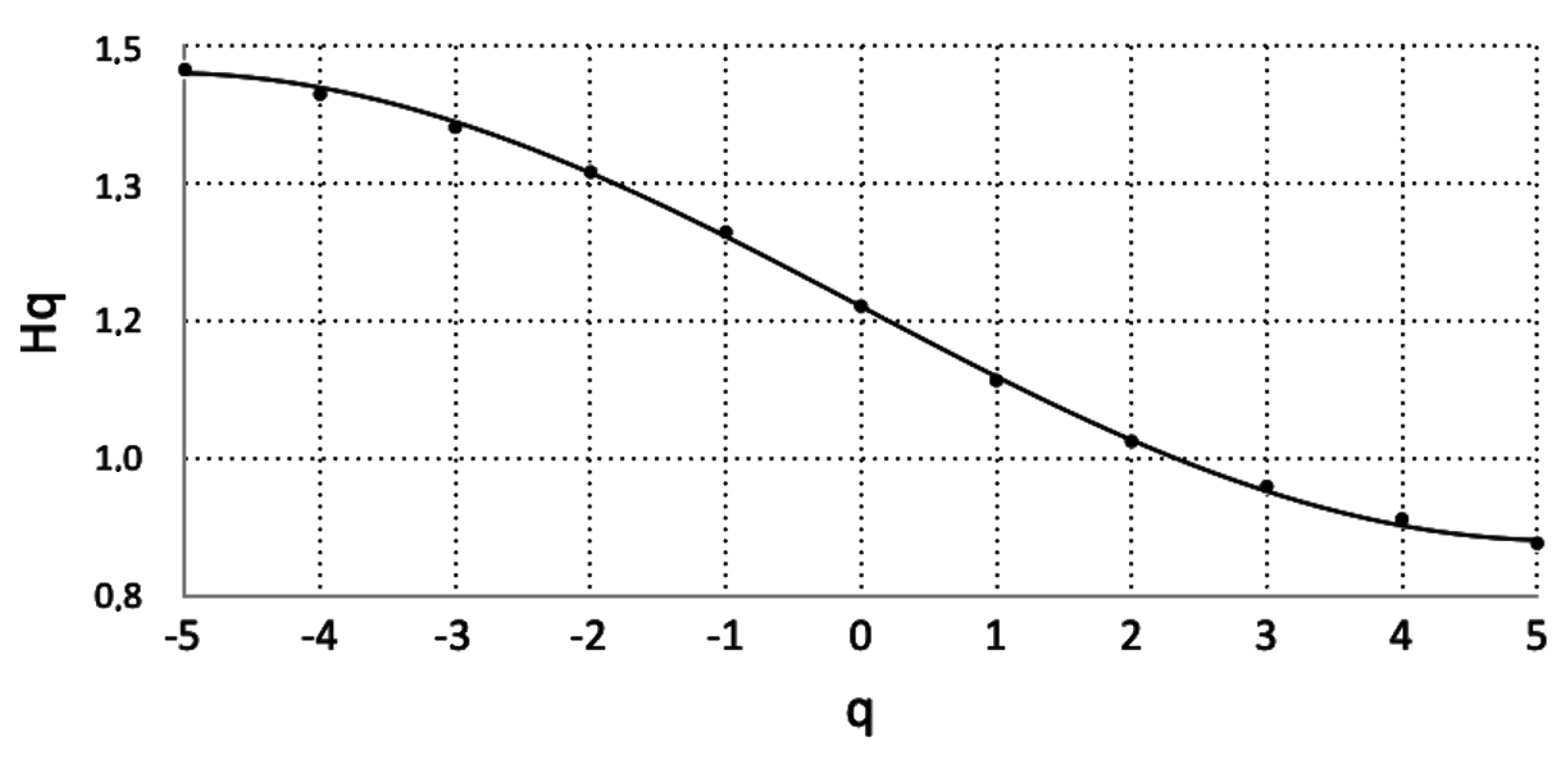
Figure 2 presents a typical curve of the variation in the generalised Hurst exponent, h q , with parameter q. The example case of Figure 2 corresponds to a two-month window with the start date 28 July 2007 and refers to the data from the AGP station. The reader may recall from Table 1 that the AGP is a Suburban-Background station. As mentioned in Section 1 and in the previous related papers for the GAA [30,31,32], this two-month window is typical for a fractal and entropy analysis of the PM10 time series of the GAA with the sliding window technique. Figure 2 is quite representative of the variation in h q versus q. The slight differences between the segments of all the other date-periods occur only in the value range of h q . It is very interesting that the curve of Figure 2 is similar to the corresponding plots of the generalised Hurst exponents reported in the other related publications [36,41,56] and, especially, regarding the air pollution series [57] and PM series [26]. The reader may also recall that h q = 2 is the classical Hurst exponent and the corresponding logarithmic plot is the typical DFA diagram [35,36,36]. As emphasised already, the DFA and Hurst exponent analysis through the R / S (case q = 2 ) has been implemented already [30,31]. According to the reported results in these publications, the special case q = 2 is significant in terms of the analysis of the PM10 time series in the GAA, Greece. The reader should note in relation that the case q = 2 refers to a monofractal analysis. When multifractals are employed, importantly, the generalised Hurst exponent ( h q ) shows a dependency on q. This implies that there is different scaling behaviour between the small and the large fluctuations. The reader should emphasise in reference to Figure 2 that the negative q values correspond to the small fluctuations, whereas the positive, to the large fluctuations. The non-symmetric curve of Figure 2 indicates a larger intensity of the small fluctuations in comparison to the large ones. Indeed, from q = −5 to q = 0, the h q values fall from approximately 1.5 to 1.2 (0.3 change), whereas from q = 0 to q = 3, the fall is from 1.2 to about 1 and then a plateau up to q = 5. These findings imply noteworthy multifractal behaviour. Because this was observed in all the cases studied, it can be concluded that the corresponding series of this paper exhibit multifractal patterns. This finding justifies a posteriori the usefulness of the multifractal approach, without cancelling the results of the monofractal analysis. In the opinion of the authors, the monofractal analysis provides an average view of the related phenomena; however, simultaneously, it is very robust in discriminating areas that may be fractal or with long-lasting interactions and, therefore, areas that are, surely, non-stochastic. Moreover, in the previous publications for the GAA, the results of the monofractal analysis were combined together (from 2 up to 13 different methods), and in this manner, very strong evidence was given regarding the underlying fractal and long-memory mechanisms. This is an advantage of the monofractal analysis of the PM10 time series in the GAA, and importantly, the novel monofractal combination approach was also checked in pre-seismic series [58]. In addition, the identified multifractality is not a priori associated with the SOC patterns identified in the PM10 time series in Nikolopoulos et al. [32]. This is why this paper initiated from the SOC periods of Table 2. The SOC periods may, practically and not theoretically, associate with fractality and, possibly, multifractality. In the opinion of the authors, this approach is the best to investigate the multifractal behaviour of lengthy data.
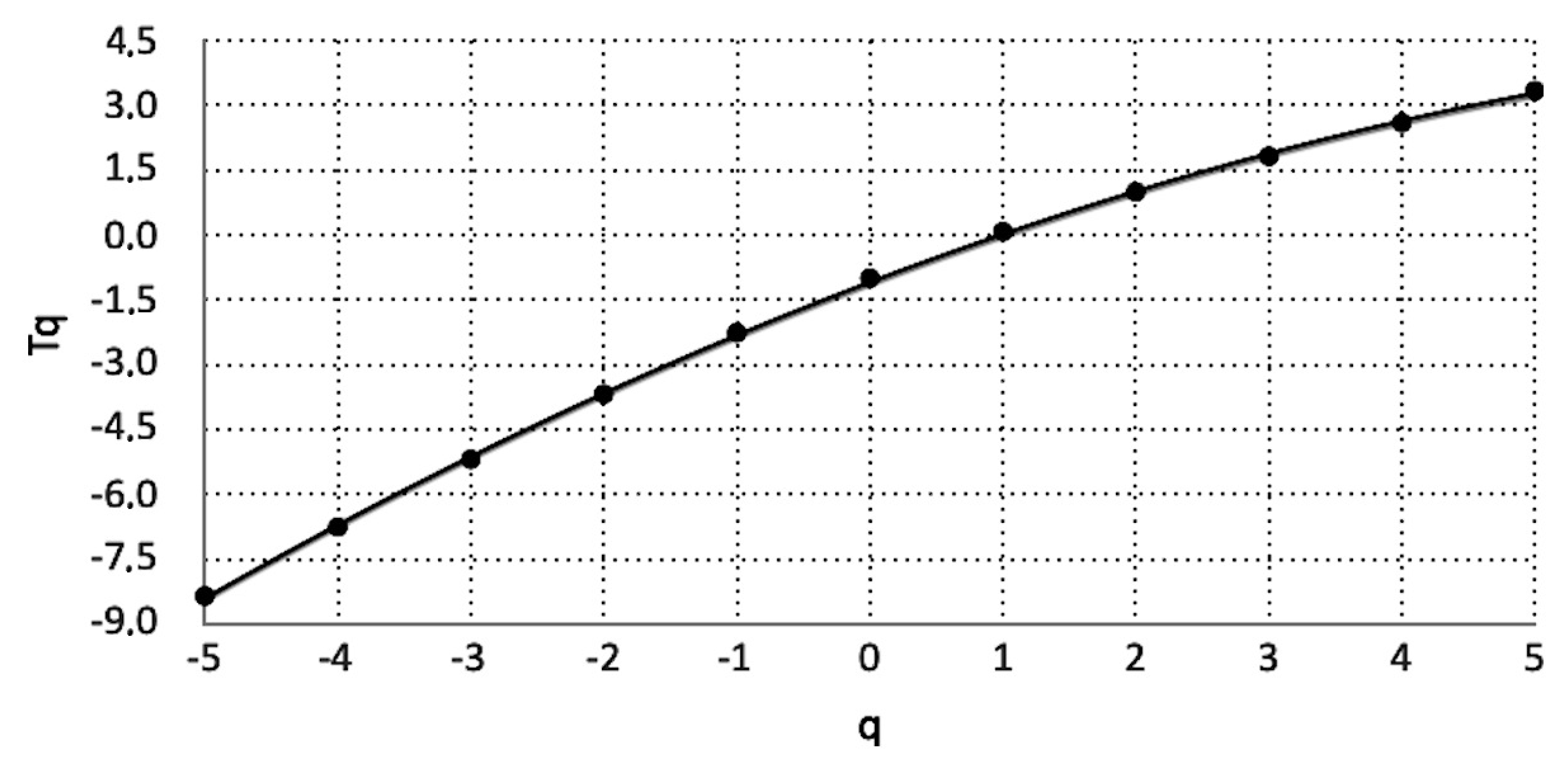
As mentioned in Section 3, the generalised Hurst exponent h q of the MFDFA of the series in Figure 2 is related to the classical scaling exponent τ q , according to Equation (8). Figure 3 presents the variation in the classical scaling exponent τ q with q. The indicated polynomial trendline corresponds to a polynomial of order 2 with equation τ q = 0.059 · q 2 + 1.17 · q 1.09 and adjusted R 2 = 0.998 . At a first glance, this non-linear association implies that there is multifractality in the corresponding two-month window and hence multiple classical Hurst exponents describe the underlying environmental system. However, a closer observation indicates a very small non-linearity coefficient ( 0.059 ). Under this view, the linear fit of the corresponding relation shows that τ q = 1.19 · q 1.17 , with the square of the square of the Spearman’s correlation coefficient R 2 = 0.986 , makes the linear approximation valid as well. This is a very important fact because it indicates, additionally to the arguments given in the previous paragraph, that the papers for PM10 in the GAA that were based on classical monofractal approximations (via the R / S analysis, DFA and fractal dimension analysis) provide solid aspects of the problem. Under a different viewpoint, as mentioned, the monofractal approximation of a multifractal system flattens the multifractal effects to an average coefficient of fractality.
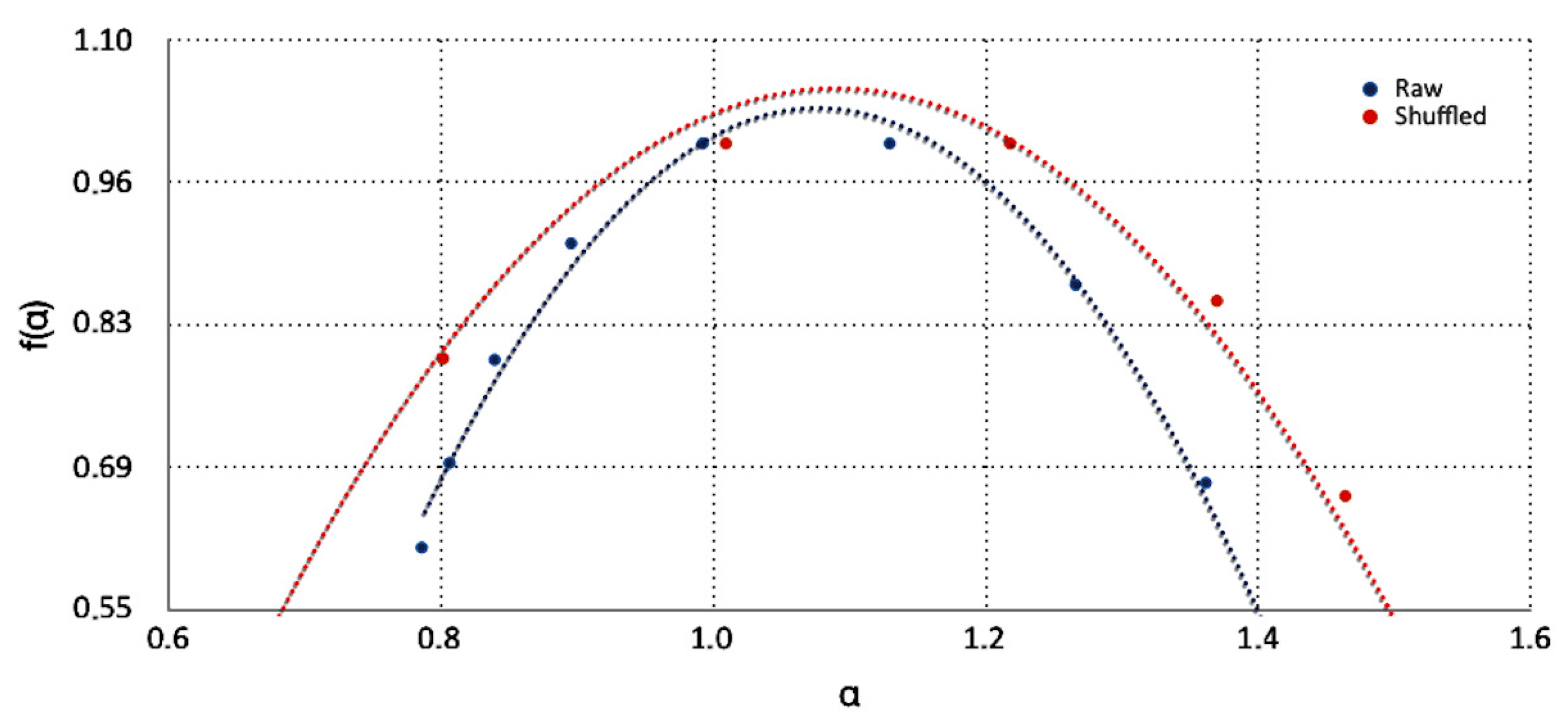
Characteristic example cases of typical multifractal plots of f α versus α are given in Figure 4, Figure 5 and Figure 6. It is very interesting that these multifractal plots are similar to those reported in other related publications [36,39,40,41,42,56], as well as in environmental pollution series [16,19,26,57]. It should be emphasised here that the sources of multifractality in the time series of these figures may originate because of the (a) existence of a broad probability function; (b) the different contributions of the small and large fluctuations to the total long-range correlations; and (c) a combination of both (a) and (b) [40,41]. The nature of the different contributions of the small and large fluctuations can be investigated by randomly shuffling the original data [36,36]. The process of shuffling removes all the long-range correlations present in the time series because the data points are rearranged in a random order. Importantly, if the shuffled data series still exhibit multifractal characteristics after the removal of the long-range correlations, then the multifractality of the underlying environmental system is due to a broad probability density function [36,36]. In this case, the generalised Hurst exponents of the original and shuffled time series will be, more or less, identical. As can be observed from Figure 4, Figure 5 and Figure 6, both raw and shuffled time series exhibit the multifractal behaviour of various maxima and widths and, additionally, shifted one to the other. It is significant that the shuffled series retain the multifractal spectrum, a fact that indicates (as aforementioned) that the source of multifractality of the PM10-generating system in the GAA is the existence of a broad probability function. The width of the spectrum indicates the degree of multifractality in the time-series data [16,19,26,39,40,41,42,57]. In these publications, the maximum value and width of the multifractal spectrum have been employed as a measure of multifractality and criticality of the multifractal behaviour. In order to calculate the differences in the characteristics of the multifractal associations between f α and α , the next mathematical procedure was followed:
1.
The derivatives of the polynomial trendlines of every association f α and α (i.e., the trendlines similar to the dotted red and blue lines in Figure 4, Figure 5 and Figure 6 and here symbolised as y = A 2 · α 2 + A 1 · α + A 0 ) were set equal to zero. Trivially, through this, the α value corresponding to the maximum is calculated (here symbolised as α m a x ) as α m a x = A 1 2 · A 2 .
2.
The maximum value of f α (symbolised as f m a x ) is calculated, trivially, as f m a x = A 2 · α 2 + A 1 · α + A 0 .
3.
Thereafter, the half-maximum ( H M ) spectrum value is calculated as y H M = f m a x 2 where y = A 2 · α 2 + A 1 · α + A 0 is the corresponding trendline.
4.
Trivially, by solving the second-order polynomial equation A 2 · α 2 + A 1 · α + A 0 = y H M , the two solutions for α ( α 1 , α 2 ) are calculated.
5.
The full width at half maximum ( F W H M ) is calculated as F W H M = | α 2 α 1 | .
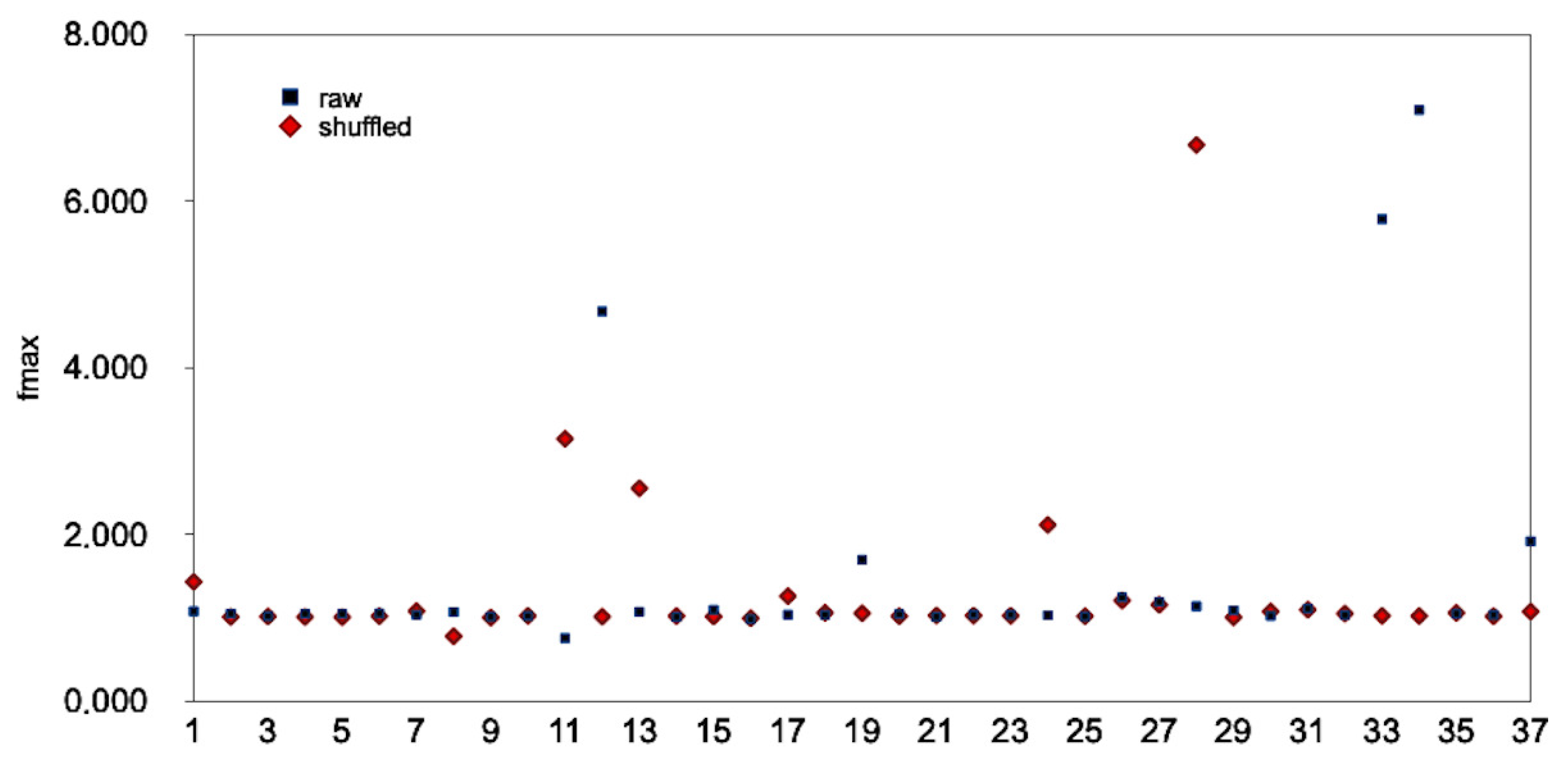
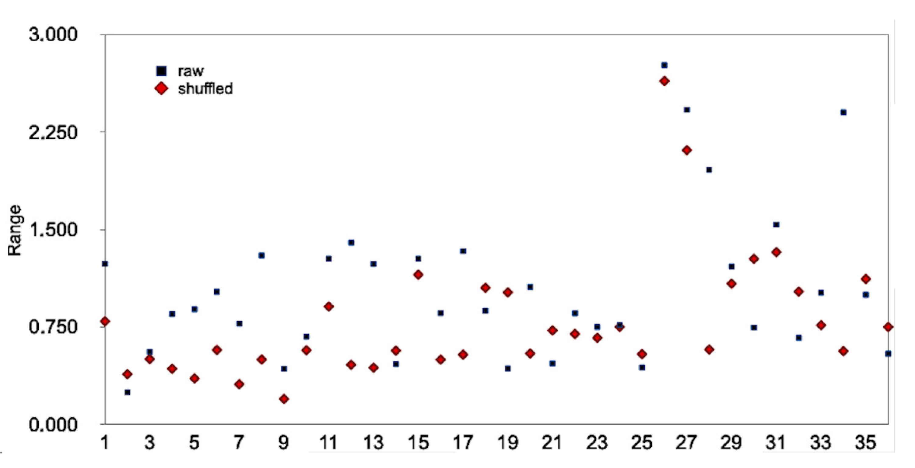
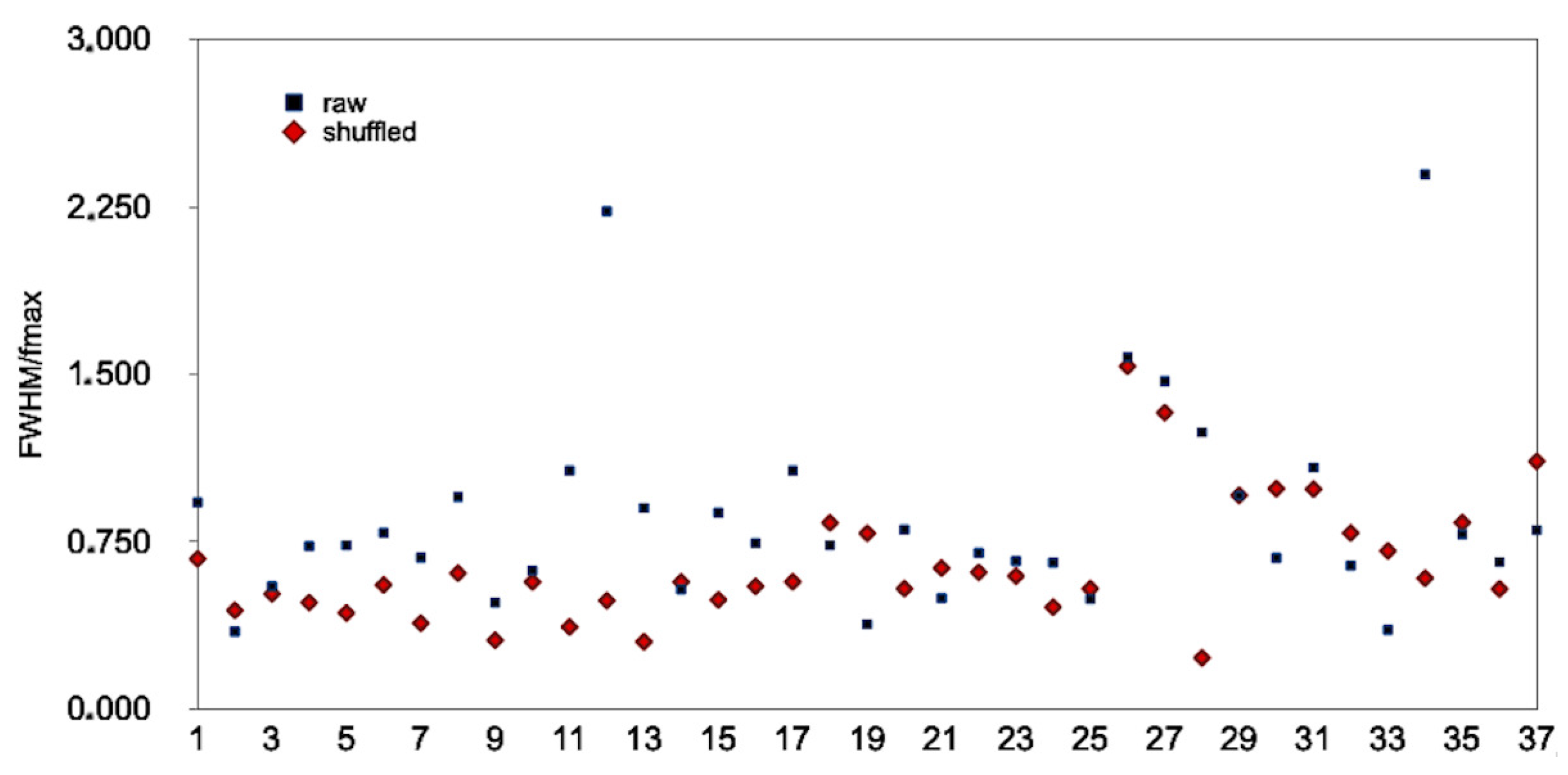
Table 3 presents the MFDFA results according to the methodology described above. In the opinion of the authors, the parameters f m a x and F W H M are the most informative measures of the multifractal characteristics of the two-month windows of Table 3. Indeed, both estimate the maximum value and width of the multifractal spectrum. Meanwhile, simultaneously, they are mathematically calculated from the fitted curves of the multifractal associations of f α versus α . Figure 7 and Figure 8 present the corresponding value distributions of f m a x and F W H M of Table 3. What is very interesting is that all f α - α curves have excellent fitting because, in all the cases, the R 2 values are quite higher than the critical value of 0.95, which has been utilised in several publications of the team. This interesting fact, significantly, is independent from the curve shape of f α - α . As a further analysis of the F W H M data of Figure 8, Figure 9 presents the distribution of the W values derived according to Equation (11). The reader may recall, in association, that the parameter W has been utilised by researchers as a measure of multifractality [39,40,56] in the same manner as F W H M is suggested to be used here. Interestingly, as long as the corresponding polynomial curves of f α versus α are not skewed, it is expected that the parameters F W H M and W are proportional, at least a priori. It is, therefore, crucial to check whether a linear association between F W H M and W actually exists. Towards this, a linear model was built in R, between F W H M and W, for both raw and shuffled series. For the raw series, the slope is (2.62 ± 0.8) with Student’s t = 3.290 (p = 0.00234) and F = 10.82 (p = 00238). For the shuffled series, the slope is (0.58 ± 0.07) with Student’s t = 8.069 (p = 2.09 × 10 9 ) and F = 65.11 (p = 2.086 × 10 9 ). An excellent linear association is observed in both cases. The higher (t, F) values of the shuffled series (and, consequently, lower corresponding p values) can be attributed to the process of shuffling, which, more or less, provides series, unbiased from potential sources of an additional disturbance. It can be supported, therefore, that both F W H M and W are good measures of multifractal broadening, with the F W H M parameter to be advantageous due to its strict calculation. For this reason, it is selected in the following as the appropriate broadening measure. In addition, from the view of R statistical density plots, all plots are bimodal, however mainly with a central main peak and a very suppressed second peak. As expected from the density plots, F W H M and W are not normally distributed. Indeed, the outputs of the R Shapiro normality test show probabilities of p = 1.128 × 10 11 for the raw data F W H M values and p = 0.0004358 for the shuffled data F W H M values, while p = 8.795 × 10 11 for the raw data W values and p = 0.001317 for the shuffled data W values. All the p values are well below the critical value of p = 0.05 and therefore the hypothesis of a normal distribution is rejected. The results are also verified by the R qq plots with deviations from the limits of normality for F W H M and W above 1 in all cases. The average F W H M equals 1.586 with the population’s standard deviation of 3.065 for the raw series and 0.770 with the population’s standard deviation of 0.346 for the shuffled series. As in the case of the linear model in R, the shuffling process produces an F W H M of a significantly lower deviation. The reader should note that, in both cases, the average and standard deviation are not representative quantities and hence give only raw outlines. On the other hand, the R statistical density plots of parameter f m a x are five-modal; however, the main peak is more than 10 times higher from all the other four modes. The probabilities of the R Shapiro normality test are 3.958 × 10 11 for the raw series W values and 2.329 × 10 11 for the shuffled series W values; namely, both are much lower than the p = 0.95 threshold. The average f m a x equals 1.481 with the population’s standard deviation of 1.360 for the raw series and average 1.333 with the population’s standard deviation of 1.012 for the shuffled series.
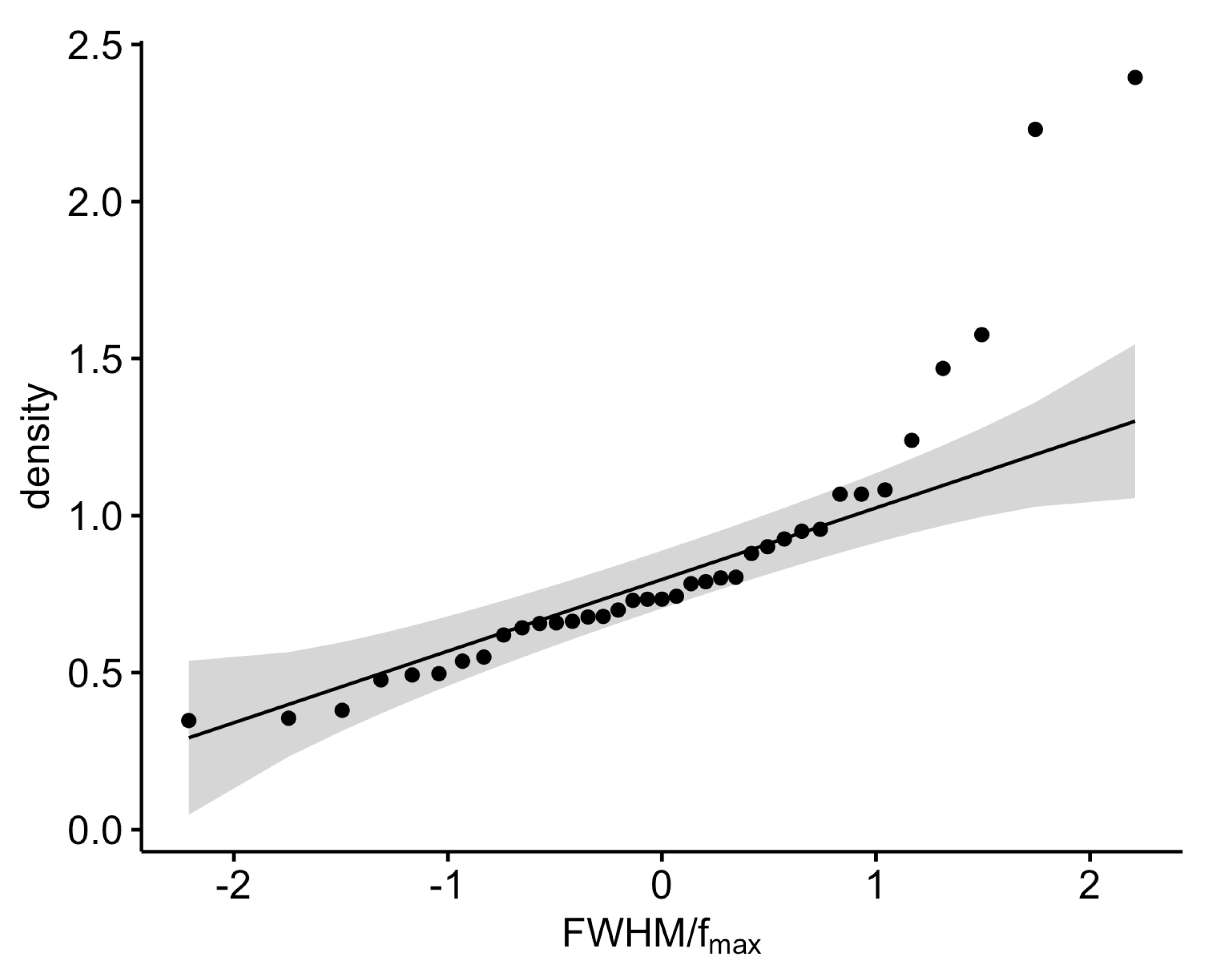
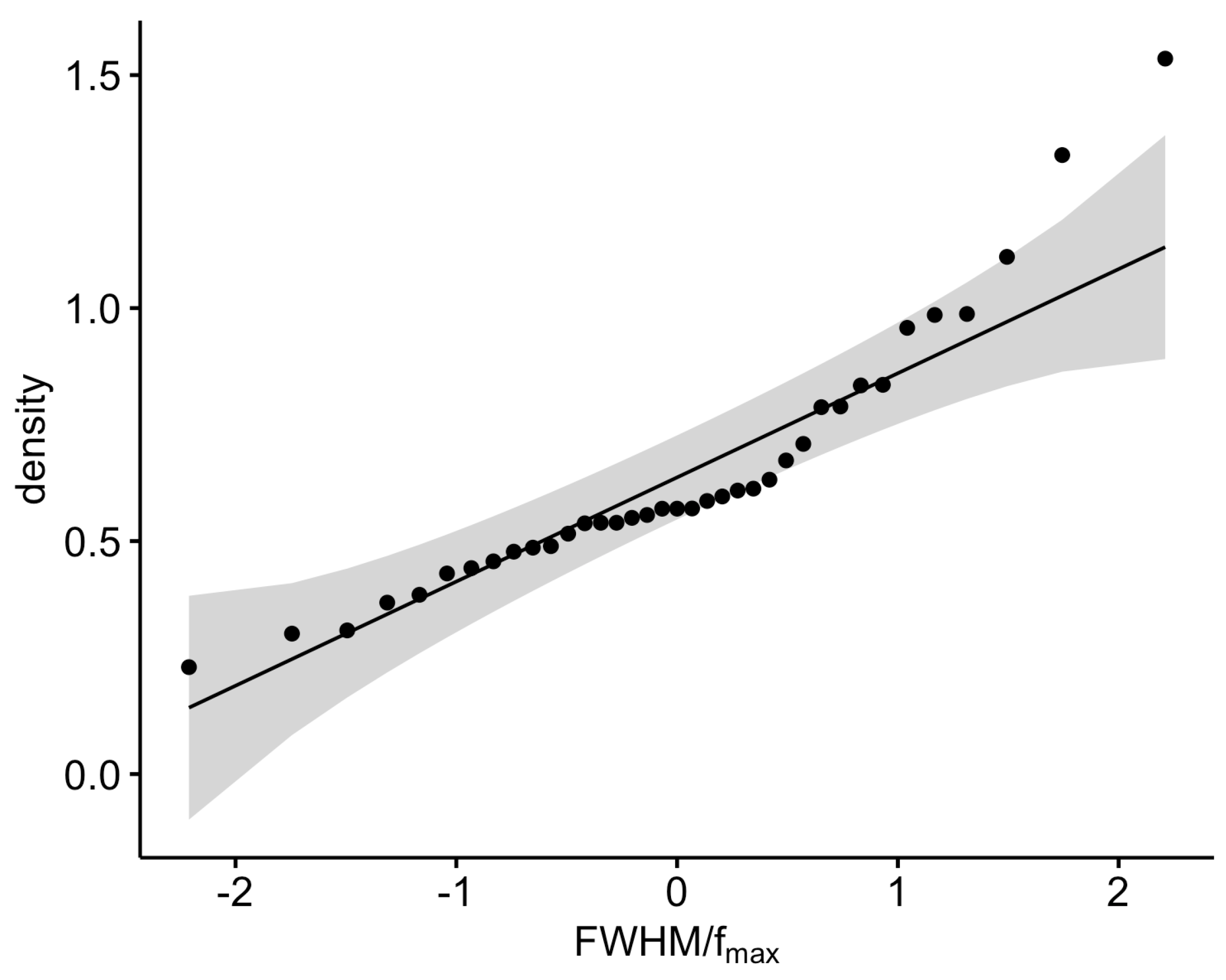
Figure 10 presents the distribution of the F W H M / f m a x values of Table 3 while Figure 11 and Figure 12 present the qq normality plots of the F W H M / f m a x values for the raw and shuffled series, respectively. According to Figure 11, five values are outside the normality limits, and these are the values with an F W H M / f m a x > 1.2. For the case of Figure 12, the cut-off normality limit is 1.1, and outside the normality limits are three values with an F W H M / f m a x > 1.1. Table 4 presents the date-periods with the multifractal characteristics out of the normality limits. The reader should focus on the fact that in these date-periods, the following are valid: (a) the PM10 system is out of stochastic behaviour; (b) the BE is below 2.0 and the TE is below 1.18; (c) points a and b are commonly found by three or more monitoring stations of Table 1; and (d) F W H M / f m a x > 1.2 for the raw series and F W H M / f m a x > 1.1 for the shuffled series. It is very important to emphasise that during these date-periods, the PM10 system is well away from randomness, exhibits SOC traces, has fractal trends and shows extraordinary multifractal behaviour. Therefore, in these date-periods, the critical and SOC and multifractal evidence is very rigid. Very importantly, in the date-period 8 January 2015, the F W H M / f m a x is out of all the thresholds, simultaneously, for the raw and shuffled series for both the AGP and LYK stations. Most significantly, the above date-period of 8 January 2015 has been reported in Nikolopoulos et al. [32] as one of the three most significant date-periods where the PM10 system is out of any threshold and, therefore, the scientific justifications for the combined fractal, SOC and multifractal trends are of the highest value. The reader should reflect on this last finding of this analysis. The combined facts coincided with the previous publications fully for one date-period and the data of one station. The background analysis however employed the fractal and critical behaviour of the data of other stations and of three stations in combination. Such data have been presented and emphasised.
In many parts of this paper, the viewpoint of the authors regarding the fractal, SOC and multifractal behaviour of the PM10 system of the GAA has been expressed under various different aspects so as to stress on the main fact: A single finding of a fractal, SOC or multifractal behaviour is significant, but only through a combination of many different techniques may incontrovertible evidence be supported. All the partial multifractal data are therefore of importance because it is a non-trivial behaviour of the PM10 series in general. The date-period 8 January 2015 for the AGP station is by far the period with the highest accuracy, supporting it as the one with multifractal, fractal and SOC trends.
As a final step regarding the multifractal nature of the PM10 system of the GAA, the sliding window MFDFA results are given in all the sub-figures of Figure 13. The generation of these sub-figures necessitated the design of special new software and a significant amount of additional calculations. In the related literature (see the example cases of Telesca et al. [39,40,41,56]), the sliding window MFDFA represents the final phase of the analysis of the multifractals, in the opinion of the authors of course. Figure 13 presents three key generalised Hurst exponents of all the series in this paper with a window of four months. The main q’s are given: q = 0, q = 2 and q = 5. These values are positive and hence, as mentioned, refer to the large variations. From the data given already, q = 0 is the cut-off point between the small and large fluctuations. The value q = 2 refers to the monofractal analysis as in all the previous papers. Finally, q = 5 is an upper value that is usually selected. The four-month window is chosen to combine the two-month windows of the analysis of the main core of this paper and to include more values so as to present additional data. Significant variations can be observed. The q = 0 time variations are higher than the corresponding ones for q = 5. The classical Hurst exponents (q = 2) are intermediate. As expressed in a previous publication [59], the q = 2 values above 1 or below 0 yield to the saturation of the corresponding fractal dimension (to 2 and 0, respectively). Therefore, these values may be considered as h ( q = 2 ) = 1 and h ( q = 2 ) = 0, respectively. It is also very interesting that certain periods with great plateaus are observed in the values of the generalised Hurst exponents in Figure 13. This is more prolonged in the MAR and THR series. In these plateau periods, the main core of the classical Hurst exponents are around 0.5. This is very significant because, in these periods, the related series are random, namely stochastic and, hence, of a statistical description. The reader may recall that the MAR station is Urban-Traffic, whereas the THR station is Suburban-Background. Therefore, the sliding window MFDFA variations seem to be independent from the type of the station. The reader should draw their attention to the following fact. It is indicated by other researchers, e.g., [60], that the differentiations in the window parameters yield to significant over- or under-estimations in the Hurst exponents. In all the analysis, the two-month window is adopted with the exception of the MFDFA sliding window results where four-month windows were used. More or less, variations are observed in all the generalised Hurst exponents of Figure 13, where the main core of the estimations refer to non-fractal and, possibly, stochastic–statistical behaviour.
It can be supported from all the analysis of this paper that the PM10 system of the GAA has several scattered parts in which fractal, SOC and multifractal patterns are addressed, and this is a new insight, at least, in view of the employed methodology. The most important finding is the date-period 8 January 2015 for the AGP station because the related evidence of fractality, multifractality and self-organised criticality is of the highest value. The results of this paper in the field of fractal and SOC analysis combines well with the results of all the recent related publications in the field of urban pollution PM10 data, providing new views for the non-stochastic and multifractal phenomena that govern the related atmospheric physics.

5. Conclusions

This paper reports the multifractal characteristics of a 17-year PM10 time series from five stations in the Greater Athens Area, Greece. The design and implementation of this study is a novel combination methodology which counts the multifractal properties calculated with a multifractal detrended fluctuation analysis applied in key periods. These key periods comprise 11 different date-periods of two-month windows for which the PM10 system is out of stochastic behaviour and has Shannon entropy and Tsallis entropy values below the critical thresholds, and all these are addressed simultaneously by at least three different monitoring stations. Accounting for the different stations per date, the total dataset of the different multifractal characteristics consists of 74 different two-month windows, 37 for the raw series and 37 for the shuffled series. All these two-month key periods were addressed in a very recent combination study conducted by the team and are considered as showing very strong evidence regarding the SOC and fractal behaviour of the PM10 system. The multifractal detrended fluctuation analysis showed that multifractal characteristics are present in all key periods. This paper reports the generalised and classical Hurst exponents and the f α versus α plots for the raw and shuffled series. All the f α versus α plots are fitted to polynomials and, from these, the parameters F W H M and f m a x are calculated and reported. The scatter plots of F W H M , f m a x and F W H M / f m a x are presented for all 74 two-month series. The statistics with R are reported for these parameters. Based on the results of the statistical analysis of the multifractal parameters, F W H M / f m a x is suggested as the best quantity to describe the results from the multifractal detrended fluctuation analysis. Analysing the outliers of the multifractal properties, five date-periods are found exhibiting extraordinary multifractal behaviour. From these, the date 8 January 2015 had extraordinary multifractal behaviour for the raw and shuffled series and for both the AGP and LYK stations. The most important finding is that this date was also identified as one between three date-periods in the most recent combination study of the team. The results and this last significant finding provide very strong evidence regarding the multifractal behaviour of the PM10 air pollution time series. Finally, the sliding window MFDFA results are given for the data of all the stations.

Author Contributions

Conceptualisation, D.N. and A.A.; methodology, D.N. and E.P.; software, D.N. and A.A.; formal analysis, D.N., E.P. and P.Y.; investigation, E.P. and K.M.; resources, K.M.; data curation, D.N. and A.A.; writing—original draft preparation, D.N., A.A., E.P. and K.M.; writing—review and editing, P.Y. and K.M.; visualisation, D.N.; supervision, D.N.; project administration, D.N. All authors have read and agreed to the published version of the manuscript.

Funding

This research received no external funding.

Institutional Review Board Statement

Not applicable.

Informed Consent Statement

Not applicable.

Data Availability Statement

Not applicable.

Conflicts of Interest

The authors declare no conflict of interest.

References

  1. European-Environment-Agency (Ed.) Air Quality Concentrations; EEA: Copenhagen, Denmark, 2021. [Google Scholar]
  2. World-Health-Organisation (Ed.) Ambient Air Pollution: A Global Assessment of Exposure and Burden of Disease; WHO—WHO Regional Office for Europe: Copenhagen, Denmark, 2021.
  3. Sicard, P.; Agathokleous, E.; De Marco, A.; Paoletti, E.; Calatayud, V. Urban population exposure to air pollution in Europe over the last decades. Environ. Sci. Eur. 2021, 33, 28. [Google Scholar] [CrossRef] [PubMed]
  4. Bendtsen, K.M.; Bengtsen, E.; Saber, A.T.; Vogel, U. A review of health effects associated with exposure to jet engine emissions in and around airports. Environ. Health 2021, 20, 7–9. [Google Scholar] [CrossRef] [PubMed]
  5. Pegoraro, V.; Heiman, F.; Levante, A.; Urbinati, D.; Peduto, I. An Italian individual-level data study investigating on the association between air pollution exposure and Covid-19 severity in primary-care setting. BMC Public Health 2021, 21, 902. [Google Scholar] [CrossRef] [PubMed]
  6. Solimini, A.; Filipponi, F.; Fegatelli, D.A.; Caputo, B.; De Marco, C.M.; Spagnoli, A.; Vestri, A.R. A global association between Covid-19 cases and airborne particulate matter at regional level. Sci. Rep. 2021, 11, 6256. [Google Scholar] [CrossRef]
  7. Sanduijav, C.; Ferreira, S.; Filipski, M.; Hashida, Y. Air pollution and happiness: Evidence from the coldest capital in the world. Ecol. Econom. 2021, 187, 107085. [Google Scholar] [CrossRef]
  8. Wang, Z.; Lu, F.; di He, H.; Lu, Q.C.; Wang, D.; Peng, Z.R. Fine-scale estimation of carbon monoxide and fine particulate matter concentrations in proximity to a road intersection by using wavelet neural network with genetic algorithm. Atmos. Environ. 2015, 104, 264–272. [Google Scholar] [CrossRef]
  9. Sefidmazgi, G.; Sayemuzzaman, M.; Homaifar, M.; Jha, M.K.; Liess, S. Trend analysis using non-stationary time series clustering based on the finite element method. Nonlinear Process. Geophys. 2014, 21, 605–615. [Google Scholar] [CrossRef] [Green Version]
  10. Maheswaran, R.; Khosa, R. Wavelet Volterra Coupled Models for forecasting of nonlinear and non–stationary time series. Neurocomputing 2015, 149, 1074–1084. [Google Scholar] [CrossRef]
  11. Moustris, K.P.; Ziomas, I.C.; Paliatsos, A.G. 3-Day-Ahead Forecasting of Regional Pollution Index for the pollutants NO2, CO, SO2 and O3 using Artificial Neural Networks in Athens, Greece. Water Air Soil. Pollut. 2010, 224, 29–43. [Google Scholar] [CrossRef]
  12. Moustris, K.P.; Nastos, P.T.; Larisssi, I.K.; Paliatsos, A.G. Application of Multiple Linear Regression Models and Artificial Neural Networks on the surface ozone forecast in the greater Athens area, Greece. Adv. Meteorol. 2012, 2012, 1–8. [Google Scholar] [CrossRef]
  13. Moustris, K.P.; Larisssi, I.K.; Nastos, P.T.; Koukouletsos, K.V.; Paliatsos, A.G. Development and Application of Artificial Neural Network Modeling in Forecasting PM10 Levels in a Mediterranean City. Water Air Soil Pollut. 2013, 224, 1634. [Google Scholar] [CrossRef]
  14. Moustris, K.P.; Proias, G.T.; Larisssi, I.K.; Nastos, P.T.; Koukouletsos, K.V.; Paliatsos, A.G. Air quality prognosis using artificial neural networks modeling in the urban environment of Volos, Central Greece. Fres. Environ. Bull. 2014, 13, 2967–2975. [Google Scholar]
  15. Moustris, K.; Petraki, E.; Ntourou, K.; Priniotakis, G.; Nikolopoulos, D. Spatiotemporal Evaluation of PM10 Concentrations within the Greater Athens Area, Greece. Trends, Variability and Analysis of a 19 Years Data Series. Environments 2020, 7, 85. [Google Scholar] [CrossRef]
  16. Dong, Q.; Wang, Y.; Li, P. Multifractal behavior of an air pollutant time series and the relevance to the predictability. Environ. Pollut. 2017, 222, 444–457. [Google Scholar] [CrossRef] [PubMed]
  17. Varotsos, C.; Ondov, J.; Efstathiou, M. Scaling properties of air pollution in Athens, Greece and Baltimore. Md. Atmos. Environ. 2005, 39, 4041–4047. [Google Scholar] [CrossRef]
  18. Kai, S.; Chun-qiong, L.; Nan-shan, A.; Xiao-hong, Z. Using three methods to investigate time-scaling properties in air pollution indexes time series. Nonlinear Anal. Real World Appl. 2008, 9, 693–707. [Google Scholar] [CrossRef]
  19. Liu, Z.; Wang, L.; Zhu, H. A time-scaling property of air pollution indices: A case study of Shanghai. China Atmos. Pollut. Res. 2015, 6, 886–892. [Google Scholar] [CrossRef]
  20. Lee, C.K.; Juang, L.C.; Wang, C.C.; Liao, Y.Y.; Yu, C.C.; Liu, Y.C.; Ho, D.S. Scaling characteristics in ozone concentration time series (OCTS). Chemosphere 2006, 62, 934–946. [Google Scholar] [CrossRef]
  21. Windsor, H.L.; Toumi, R. Scaling and persistence of UK pollution. Atmos. Environ. 2001, 35, 4545–4556. [Google Scholar] [CrossRef]
  22. Weng, Y.C.; Chang, N.B.; Lee, T.Y. Nonlinear time series analysis of ground-level ozone dynamics in Southern Taiwan. J. Environ. Manag. 2008, 87, 405–414. [Google Scholar] [CrossRef]
  23. Chelani, A.B. Predicting chaotic time series of PM10 concentration using artificial neural network. J. Environ. Stud. 2005, 62, 181–191. [Google Scholar] [CrossRef]
  24. Chelani, A.B. Statistical persistence analysis of hourly ground level ozone concentrations in Delhi. Atmos. Res. 2009, 92, 244–250. [Google Scholar] [CrossRef]
  25. Chelani, A.B. Persistence analysis of extreme CO, NO2 and O3 concentrations in ambient air of Delhi. Atmos. Res. 2012, 108, 128–134. [Google Scholar] [CrossRef]
  26. Xue, Y.; Pan, W.; Lu, W.z.; He, H.D. Multifractal nature of particulate matters (PMs) in Hong Kong urban air. Sci. Total Environ. 2015, 532, 744–751. [Google Scholar] [CrossRef]
  27. Yuval; Broday, D.M. Studying the time scale dependence of environmental variables predictability using fractal analysis. Environ. Sci. Technol. 2010, 44, 4629–4634. [Google Scholar] [CrossRef]
  28. Pacheco, P.R.; Parodi, M.C.; Mera, E.M.; Salini, G.A. Variables meteorologicas y niveles de concentracion de material particulado de 10 μm en Andacollo, Chile: Un estudio de dispersioy entropias. Inf. Tecnol. 2020, 31, 171–182. [Google Scholar] [CrossRef]
  29. Du, W.; Wang, J.; Wang, Z.; Lei, Y.; Huang, Y.; Liu, S.; Wu, C.; Ge, S.; Chen, Y.; Bai, K.; et al. Influence of COVID-19 lockdown overlapping Chinese Spring Festival on household PM2.5 in rural Chinese homes. Chemosphere 2021, 278, 130406. [Google Scholar] [CrossRef]
  30. Nikolopoulos, D.; Moustris, K.; Petraki, E.; Koulougliotis, D.; Cantzos, D. Fractal and Long-Memory Traces in PM10 Time Series in Athens, Greece. Environments 2019, 7, 29. [Google Scholar] [CrossRef] [Green Version]
  31. Nikolopoulos, D.; Moustris, K.; Petraki, E.; Cantzos, D. Long-memory traces in PM10 time series in Athens, Greece: Investigation through DFA and R/S analysis. Meteorol. Atmos. Phys. 2021, 133, 261–279. [Google Scholar] [CrossRef]
  32. Nikolopoulos, D.; Alam, A.; Petraki, E.; Papoutsidakis, M.; Yannakopoulos, P.; Moustris, K.P. Stochastic and Self-Organisation Patterns in a 17-Year PM10 Time Series in Athens. Entropy 2021, 23, 307. [Google Scholar] [CrossRef]
  33. Hellenic-Statistical-Authority-HSA. Population-Housing Census; HSA: Singapore, 2011. [Google Scholar]
  34. Hellenic-National-Meteorological-Service. Climatic Data for Selected Stations in Greece. Available online: http://www.hnms.gr/emy/en/climatology/climatology_city?perifereia=Attiki&poli=Athens_Hellinikon/ (accessed on 1 January 2020.).
  35. Chen, Z.; Ivanov, P.; Hu, K.; Stanley, H. Effect of nonstationarities on detrended fluctuation analysis. Phys. Rev. E 2002, 65, 1–15. [Google Scholar] [CrossRef]
  36. Kantelhardt, J.W.; Zschiegner, S.A.; Koscielny-Bunde, E.; Havlin, S.; Bunde, A.; Stanley, H. Multifractal detrended fluctuation analysis of nonstationary time series. Phys. Stat. Mech. Appl. 2002, 316, 87–114. [Google Scholar] [CrossRef] [Green Version]
  37. Salat, H.; Murcio, R.; Arcaute, E. Multifractal methodology. Phys. A 2017, 473, 467–487. [Google Scholar] [CrossRef]
  38. Olemskoi, A.I.; Vadym, N.; Borysiuk, I.A.; Bagdasaryan, S.A. Multifractal analysis for the time series related to economic systems. J. Nano Electr. Phys. 1999, 1, 82–88. [Google Scholar]
  39. Telesca, L.; Lapenna, V.; Vallianatos, F. Monofractal and multifractal approaches in investigating scaling properties in temporal patterns of the 1983–2000 seismicity in the Western Corinth Graben, Greece. Phys. Earth Planet. Int. 2002, 131, 63–79. [Google Scholar] [CrossRef]
  40. Telesca, L.; Lapenna, V.; Macchiato, M. Mono- and multi-fractal investigation of scaling properties in temporal patterns of seismic sequences. Chaos Solit. Fractals 2004, 19, 1–15. [Google Scholar] [CrossRef]
  41. Telesca, L.; Lapenna, V.; Macchiato, M. Multifractal fluctuations in seismic interspike series. Phys. A 2005, 354, 629–640. [Google Scholar] [CrossRef] [Green Version]
  42. Telesca, L.; Lasaponara, R. Vegetational patterns in burned and unburned areas investigated by using the detrended fluctuation analysis. Phys. A 2006, 368, 531–535. [Google Scholar] [CrossRef]
  43. Ghosh, D.; Deb, A.; Dutta, S.; Sengupta, R. Multifractality of radon concentration fluctuation in earthquake related signal. Fractals 2012, 20, 33–39. [Google Scholar] [CrossRef]
  44. Alam, A.; Wang, N.; Zhao, G.; Mehmood, T.; Nikolopoulos, D. Long-lasting patterns of radon in groundwater at Panzhihua, China: Results from DFA, fractal dimensions and residual radon concentration. Geochem. J. 2019, 53, 341–358. [Google Scholar] [CrossRef]
  45. Nikolopoulos, D.; Petraki, E.; Marousaki, A.; Potirakis, S.; Koulouras, G.; Nomicos, C.; Panagiotaras, D.; Stonhamb, J.; Louizi, A. Environmental monitoring of radon in soil during a very seismically active period occurred in South West Greece. J. Environ. Monit. 2012, 14, 564–578. [Google Scholar] [CrossRef]
  46. Nikolopoulos, D.; Petraki, E.; Vogiannis, E.; Chaldeos, Y.; Giannakopoulos, P.; Kottou, S.; Nomicos, C.; Stonham, J. Traces of self-organisation and long-range memory in variations of environmental radon in soil: Comparative results from monitoring in Lesvos Island and Ileia (Greece). J. Radioanal. Nucl. Chem. 2014, 299, 203–219. [Google Scholar] [CrossRef]
  47. Nikolopoulos, D.; Petraki, E.; Nomicos, C.; Koulouras, G.; Kottou, S.; Yannakopoulos, P.H. Long-Memory Trends in Disturbances of Radon in Soil Prior ML=5.1 Earthquakes of 17 November 2014 Greece. J. Earth Sci. Clim. Chang. 2015, 6, 1–11. [Google Scholar]
  48. Nikolopoulos, D.; Valais, I.; Michail, C.; Bakas, A.; Fountzoula, C.; Cantzos, D.; Bhattacharyya, D.; Sianoudis, I.; Fountos, G.; Yannakopoulos, P.H.; et al. Radioluminescence properties of the CdSe/ZnS Quantum Dot nanocrystals with analysis of long-memory trends. Radiat. Meas. 2016, 92, 19–31. [Google Scholar] [CrossRef] [Green Version]
  49. Nikolopoulos, D.; Cantzos, D.; Petraki, E.; Yannakopoulos, P.H.; Nomicos, C. Traces of long-memory in pre-seismic MHz electromagnetic time series-Part1: Investigation through the R/S analysis and time-evolving spectral fractals. J. Earth Sci. Clim. Chang. 2016, 7, 359. [Google Scholar] [CrossRef] [Green Version]
  50. Nikolopoulos, D.; Petraki, E.; Cantzos, D.; Yannakopoulos, P.H.; Panagiotaras, D.; Nomicos, C. Fractal Analysis of Pre-Seismic Electromagnetic and Radon Precursors: A Systematic Approach. J. Earth Sci. Clim. Chang. 2016, 7, 1–11. [Google Scholar]
  51. Nikolopoulos, D.; Matsoukas, C.; Yannakopoulos, P.H.; Petraki, E.; Cantzos, D.; Nomicos, C. Long-Memory and Fractal Trends in Variations of Environmental Radon in Soil: Results from Measurements in Lesvos Island in Greece. J. Earth Sci. Clim. Chang. 2018, 9, 1–11. [Google Scholar]
  52. Petraki, E.; Nikolopoulos, D.; Fotopoulos, A.; Panagiotaras, D.; Koulouras, G.; Zisos, A.; Nomicos, C.; Louizi, A.; Stonham, J. Self-organised critical features in soil radon and MHz electromagnetic disturbances: Results from environmental monitoring in Greece. Appl. Radiat. Isotop. 2013, 72, 39–53. [Google Scholar] [CrossRef]
  53. Petraki, E.; Nikolopoulos, D.; Fotopoulos, A.; Panagiotaras, D.; Nomicos, C.; Yannakopoulos, P.; Kottou, S.; Zisos, A.; Louizi, A.; Stonham, J. Long-range memory patterns in variations of environmental radon in soil. Anal. Methods 2013, 5, 4010–4020. [Google Scholar] [CrossRef]
  54. Petraki, E.; Nikolopoulos, D.; Nomicos, C.; Stonham, J.; Cantzos, D.; Yannakopoulos, P.; Kottou, S. Electromagnetic Pre-earthquake Precursors: Mechanisms, Data and Models-A Review. J. Earth Sci. Clim. Chang. 2015, 6, 1–11. [Google Scholar]
  55. Petraki, E.; Nikolopoulos, D.; Panagiotaras, D.; Cantzos, D.; Yannakopoulos, P.; Nomicos, C.; Stonham, J. Radon-222: A Potential Short-Term Earthquake Precursor. J. Earth Sci. Clim. Chang. 2015, 6, 1–11. [Google Scholar]
  56. Telesca, L.; Lapenna, V. Measuring multifractality in seismic sequences. Tectonophysics 2006, 423, 115–123. [Google Scholar] [CrossRef]
  57. He, Y.; Gu, Z.; Lu, W.; Zhang, L.; Okuda, T.; Fujioka, K.; Luo, H.; Yu, C. Atmospheric humidity and particle charging state on agglomeration of aerosol particles. Atmos. Environ. 2019, 197, 141–149. [Google Scholar] [CrossRef]
  58. Nikolopoulos, D.; Petraki, E.; Yannakopoulos, P.; Priniotakis, G.; Voyiatzis, I.; Cantzos, D. Long-Lasting Patterns in 3 kHz Electromagnetic Time Series after the ML = 6.6 Earthquake of 2018-10-25 near Zakynthos, Greece. Geosciences 2020, 10, 235. [Google Scholar] [CrossRef]
  59. Petraki, E.; Nikolopoulos, D.; Chaldeos, Y.; Koulouras, G.; Nomicos, C.; Yannakopoulos, P.H.; Kottou, S.; Stonham, J. Fractal evolution of MHz electromagnetic signals prior to earthquakes: Results collected in Greece during 2009. Geomat. Nat. Hazards Risk 2016, 7, 550–564. [Google Scholar] [CrossRef]
  60. Granero, M.S.; Segovia, J.T.; Pérez, J.G. Some comments on Hurst exponent and the long memory processes on capital markets. Phys. A 2008, 387, 543–551. [Google Scholar]
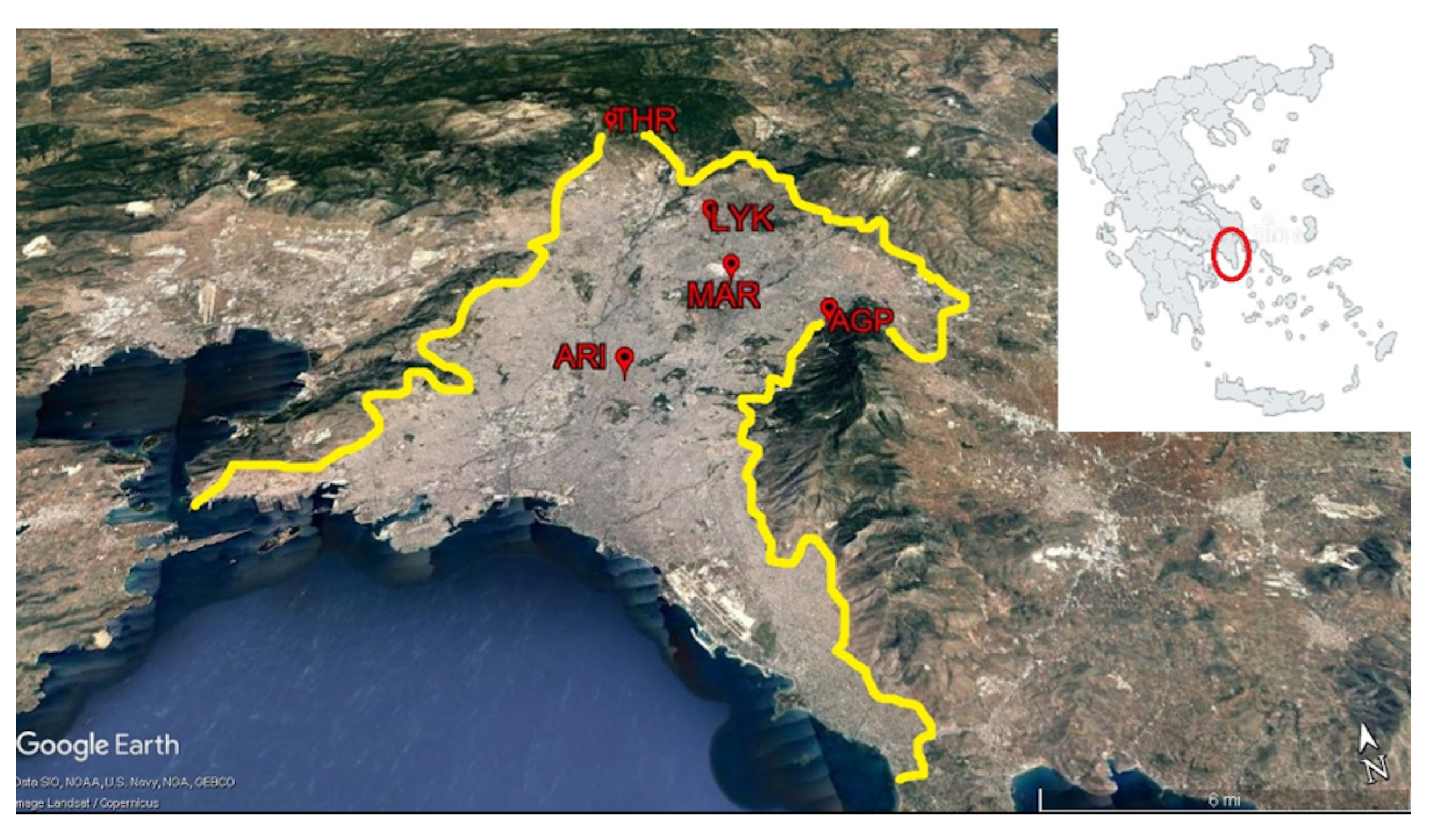
Figure 1. The map of the GAA and the location of the five air pollution monitoring stations.
Environments 10 00009 g001
Figure 2. Generalised Hurst exponent ( h q ) versus qs for the AGP monitoring station and date 28 July 2007 (case i/i = 2 of Table 2).
Environments 10 00009 g002
Figure 3. Classical scaling exponent τ q with q for the AGP monitoring station and date 28 July 2007 (case i/i = 3 of Table 2).
Environments 10 00009 g003
Figure 4. Multifractal plot of f α versus α for the THR monitoring station and date 7 July 2016 (case i/i = 11 of Table 2). Blue dots indicate the raw two-month series and the red dots the shuffled series. The dotted trendlines refer to fitted polynomial curves of order 2. For details, the reader should refer in-text.
Environments 10 00009 g004
Figure 5. Multifractal plot of f α versus α for the THR monitoring station and date 4 April 2009 (case i/i = 10 of Table 2). Blue dots indicate the raw two-month series and the red dots the shuffled series. The dotted trendlines refer to fitted polynomial curves of order 2. For details, the reader should refer in-text.
Environments 10 00009 g005
Figure 6. Multifractal plot of f α versus α for the THR monitoring station and date 6 February 2015 (case i/i = 11 of Table 2). Blue dots indicate the raw two-month series and the red dots the shuffled series. The dotted trendlines refer to fitted polynomial curves of order 2. For details, the reader should refer in text.
Environments 10 00009 g006
Figure 7. Scatter plot of f m a x values versus the i/i value of Table 2. Blue dots indicate the raw two-month series and the red dots the shuffled series.
Environments 10 00009 g007
Figure 8. Scatter plot of F W H M values versus the i/i value of Table 2. Blue dots indicate the raw two-month series and the red dots the shuffled series.
Environments 10 00009 g008
Figure 9. Scatter plot of ranges W (Equation (11)) versus the i/i value of Table 2. Blue dots indicate the raw two-month series and the red dots the shuffled series.
Environments 10 00009 g009
Figure 10. Scatter plot of F W H M / f m a x versus the i/i value of Table 2. Blue dots indicate the raw two-month series and the red dots the shuffled series.
Environments 10 00009 g010
Figure 11. QQ nomality plot of F W H M / f m a x values of Table 3 for the raw time series.
Environments 10 00009 g011
Figure 12. QQ nomality plot of F W H M / f m a x values of Table 3 for the shuffled time series.
Environments 10 00009 g012
Figure 13. Results of the sliding window MFDFA.
Environments 10 00009 g013
Table 1. The examined air pollution monitoring stations and their characteristics. Abbr. means abbreviation, Alt. means altitude above sea level (a.s.l.) and D.C. means data completeness.
Monitoring StationAbbr.LongitudeLatitudeAlt. (m)CharacterisationD.C.
AristotelousARI23°43 39 37°59 16 75Urban-Traffic85.8%
LykovrissiLYK23°47 19 38°04 04 234Suburban-Background89.2%
MaroussiMAR23°47 14 38°01 51 170Urban-Traffic82.5%
Agia ParaskeviAGP23°49 09 37°59 42 290Suburban-Background88.7%
ThrakomakedonesTHR23°45 29 38°08 36 550Suburban-Background77.2%
Table 2. Date-periods of the 11 areas (date-periods) of Nikolopoulos et al. [32] that simultaneously (a) are out of stochastic behaviour, (b) BE is below 2.0 and TE below 1.18 and (c) points a and b are commonly found by 3 or more monitoring stations of Table 1. i/i is the index value of the common date-periods.
i/iDateMonitoring Stations
1.25 March 2007AGP, ARI, MAR
2.28 July 2007AGP, LYME, MAR
3.4 April 2009AGP, ARI, LYK, THR
4.6 April 2009AGP, ARI, MAR, THR
5.7 June 2010AGP, LYK, MAR
6.26 June 2014AGP, ARI, LYK, MAR
7.27 June 2014AGP, ARI, LYK, MAR
8.8 January 2015AGP, LYK, MAR
9.2 February 2015AGP, MAR
10.6 February 2015AGP, ARI, MAR, THR
11.7 July 2016AGP, ARI, THR
Table 3. MFDFA results of the 11 date-periods of Table 2. In these date-periods, according to Nikolopoulos et al. [32], the following facts happen simultaneously: (a) the PM10 is out of stochastic behaviour, (b) BE is below 2.0 and TE below 1.18 and (c) points a and b are commonly found by 3 or more monitoring stations of Table 1. For calculations of F W H M and f m a x , the reader should refer to text. R 2 is the square of the adjusted coefficient of each fit.
DateStation Raw Shuffled
R2fmaxFWHMFWHM/ fmaxR2fmaxFWHMFWHM/ fmax
25 March 2007AGP0.9901.0801.0000.9260.9931.430.9650.673
ARI0.9991.0530.3660.3470.9991.010.450.442
MAR0.9971.0220.5620.5500.9971.020.5250.516
28 July 2007AGP0.9921.050.7680.7300.9971.010.4830.477
LYK0.9941.050.7710.7340.9971.010.4350.431
MAR0.9941.060.8340.7900.9671.020.5680.556
4 April 2009AGP0.9951.0390.7060.6790.99731.080.4170.385
ARI0.9911.0731.0190.9500.99760.780.4760.608
LYK0.9971.0170.4850.4770.99941.010.3100.308
THR0.9931.0250.6350.6200.9951.030.5850.570
6 April 2009AGP0.9900.7590.8111.0680.9963.151.1590.368
ARI0.9654.68110.4402.2300.9981.020.4930.486
MAR0.9911.0750.9690.9010.99782.560.7710.301
THR0.9921.0130.5440.5370.99541.020.5830.569
6 July 2010AGP0.9871.0980.9650.8800.99381.020.4980.489
LYK0.9990.9880.5550.7430.99241.000.5490.550
MAR0.9951.0391.0551.0680.99671.260.7200.570
26 June 2014AGP0.9931.0390.7630.7340.98991.060.8870.834
ARI0.9921.6990.6460.3800.99371.060.8320.787
LYK0.9931.0460.8410.8040.99751.020.5510.539
MAR0.9971.0160.5050.4970.99071.030.6510.632
27 June 2014AGP0.9951.0420.7290.6990.98711.030.6300.613
ARI0.9931.0400.6900.6640.99751.030.6120.596
LYK0.9941.0340.6790.6560.99632.120.9670.456
MAR0.9971.0190.5020.4930.99671.020.5510.539
8 January 2015AGP0.9851.2461.9641.5760.98291.211.8601.535
LYK0.9851.1951.7551.4690.98011.161.5381.328
MAR0.9821.1411.4151.2400.99276.681.5330.230
2 February 2015AGP0.9901.0921.0440.9560.9981.010.9650.958
MAR0.9941.0270.6960.6770.98931.081.0650.987
6 February 2015AGP0.9881.1141.2051.0820.9871.101.0840.985
ARI0.9931.0350.6650.6430.9931.050.8310.789
MAR0.9915.7892.0550.3550.99391.030.7280.709
THR0.9697.09917.0052.3950.99411.030.6010.586
7 July 2016AGP0.9931.0520.8240.7830.99291.060.8870.835
ARI0.9951.0390.6840.6590.99731.020.5500.538
THR0.9901.9211.5400.8020.99181.081.1971.110
Table 4. Date-periods of Table 2 for which: (a) the PM10 system is out of stochastic behaviour; (b) BE is below 2.0 and TE below 1.18; (c) points a and b are commonly found by 3 or more monitoring stations of Table 1; (d) F W H M / f m a x > 1.2 for the raw series or F W H M / f m a x > 1.1 for the shuffled series. Raw symbolises the F W H M / f m a x of the raw series and Shuffled of the shuffled series, respectively.
DateStationRawShuffled
6 April 2009ARI2.2300.486
8 January 2015AGP1.5761.535
8 January 2015LYK1.4691.328
6 February 2015THR2.3950.586
7 July 2016THR0.8021.110
Disclaimer/Publisher’s Note: The statements, opinions and data contained in all publications are solely those of the individual author(s) and contributor(s) and not of MDPI and/or the editor(s). MDPI and/or the editor(s) disclaim responsibility for any injury to people or property resulting from any ideas, methods, instructions or products referred to in the content.