Periodicity in Volcanic Gas Plumes: A Review and Analysis

Abstract

Persistent non-explosive passive degassing is a common characteristic of active volcanoes. Distinct periodic components in measurable parameters of gas release have been widely identified over timescales ranging from seconds to months. The development and implementation of high temporal resolution gas measurement techniques now enables the robust quantification of high frequency processes operating on timescales comparable to those detectable in geophysical datasets. This review presents an overview of the current state of understanding regarding periodic volcanic degassing, and evaluates the methods available for detecting periodicity, e.g., autocorrelation, variations of the Fast Fourier Transform (FFT), and the continuous wavelet transform (CWT). Periodicities in volcanic degassing from published studies were summarised and statistically analysed together with analyses of literature-derived datasets where periodicity had not previously been investigated. Finally, an overview of current knowledge on drivers of periodicity was presented and discussed in the framework of four main generating categories, including: (1) non-volcanic (e.g., atmospheric or tidally generated); (2) gas-driven, shallow conduit processes; (3) magma movement, intermediate to shallow storage zone; and (4) deep magmatic processes.

1. Introduction

Active volcanoes commonly exhibit persistent (i.e., continuous or quasi-continuous) emission of gases from summit vents or fumaroles (Figure 1). Persistently degassing volcanoes are typically those erupting magmas with lower silica contents—i.e., basalts, basaltic-andesites, and andesites—and thus, lower viscosities. In contrast to more silicic magmas where gas bubbles remain strongly coupled to the melt, low magma viscosities permit efficient fluid-melt separation [1,2] and allow bubbles to move independently of the melt. Once nucleated, bubbles in magma can grow either by diffusion of volatiles into the bubble, decompression, and coalescence, before either bursting at the magma surface or undergoing explosive fragmentation [3,4,5]. Volcanic gas emissions are predominantly composed of water vapor (H₂O), carbon dioxide (CO₂), and sulfur dioxide (SO₂, or in reduced form, hydrogen sulfide, H₂S), with SO₂ being the easiest to resolve against background atmospheric concentrations and therefore, generally the target gas used for emissions measurements [6]. Present generally in trace quantities are halogen compounds such as chlorine, fluorine, bromine, and iodine, the latter of which is highly reactive in the atmosphere forming gaseous species such as bromine monoxide (BrO), and iodine monoxide (IO) [7,8,9].

The relative ease of measuring SO₂, compared to other major gas species, has meant that this gas is often the target for remote sensing. Prior to the development of ultra violet (UV) camera technology [10,11], measurement techniques were constrained by sampling rate and therefore lacked the temporal resolution to detect rapid changes in SO₂ flux. For example, Differential Optical Absorption Spectroscopy (DOAS) could at best achieve resolutions of minutes because of the need to traverse or scan gas plumes [12,13,14]. Now, with the advent of UV cameras, which generally acquire at frequencies approaching 1 Hz, periodic components (oscillations) in gas flux are resolvable on timescales of 10 s to 1000 s [6,15,16,17,18,19].

The existence of longer timescale periodicity in volcanic outgassing on the order of days to months was first identified at well-studied systems with long monitoring timeseries, e.g., Kīlauea, Hawaii [20] and Soufriere Hills Volcano, Montserrat [21]. Whilst low frequency periodic components are widely thought to originate from deep processes related to large-scale magma movement [22,23], high frequency signals can be derived from a wide range of potential drivers [16]. The causes and implications of short-period cycles have yet to be compared in detail across volcanoes.

The detection of periodic behavior is not restricted to SO₂ flux measurements alone, and periodicity can also be identified in timeseries of molar gas ratios [16,24,25,26,27]. Open-Path Fourier Transform Infrared Spectroscopy (OP-FTIR) can capture high temporal resolution datasets of molar gas ratios for a broad range of gases, including trace species such as chlorine [28,29,30,31,32]. In combination with thermodynamic models of volatile solubility, molar gas ratios can be directly related to the pressure (depth) of gas-melt separation and are therefore critical to the identification and tracking of new magma inputs and their subsequent ascent through the shallow magmatic system [33,34,35,36] or to discriminate between redox- and solubility-driven processes [24,37].

This review summarizes the literature associated with the full range of currently resolvable periodicities within volcanic degassing timeseries, starting with an overview of the methods for detecting periodicity.

2. Methods for Detecting Periodicity

2.1. Spectral Analysis

The presence of periodicity within volcanic gas datasets is quantified based on the principle of spectral analysis, or frequency analysis, whereby timeseries data are decomposed into a series of waves of known wavelength and amplitude, to determine the strength of different frequencies within discrete datasets. Spectral analysis is commonly performed using one of two main groups of techniques (summarized in

Table 1. A summary of techniques used for identifying periodicity and their ideal usage. FFT refers to the Fast Fourier Transform.

Technique	Ideal Use
Autocorrelation	Stationary periodicity, one clear and dominant period
Welch’s (FFT)	Non-stationary periodicity, but approx. stationary within window, requires prior knowledge of target periodicity timescale
Thomson’s Multitaper (FFT)	Stationarity required within an individual analysis window; but, can visualise non-stationary periodicity when employed in the form of the short-term Fourier transform (STFT) moving window method. Requires no prior knowledge of target periodicity timescale
Lomb-Scargle (FFT)	Non-stationary periodicity, for datasets with missing data points
Continuous Wavelet Transform	Non-stationary, good for visualizing temporal stability and strength of multiple concurrent periodicities. Requires no prior knowledge on the signal generating process.

): the fast Fourier transform (FFT) [38,39,40,41,42,43], and the wavelet transform [16,44,45,46,47,48,49]. The continuous wavelet transform (CWT) is increasingly preferred because it offers additional degrees of freedom, such that the temporal persistence of periodic components can be investigated in detail, particularly where those components exhibit non-stationary characteristics [16,19,24,48,49,50,51]. When conducting spectral analysis, we can only consider a maximum cycle length of half the dataset length; this is termed the Nyquist criterion [52]. For example, with a dataset 1000 s in length, the maximum detectable period would be 500 s. However, as this would only allow two complete periodic cycles, it is often preferable and advisable to set the cut-off at a frequency higher than the Nyquist limit, for example at three or four complete periodic cycles. This principle is applicable to all spectral analysis techniques, including the CWT. Autocorrelation, or serial correlation, has also been applied for spectral analysis, e.g., [26,53]. As part of any spectral analysis, it is important to consider errors within the input dataset, particularly considering that gas datasets can be associated with high uncertainties.

2.2. Autocorrelation

Autocorrelation is a measure of how correlated a variable is with itself across a range of lag times, using Pearson’s Product Moment Correlation [54]. Autocorrelation is highly effective, therefore, at identifying periodicities that are stationary (i.e., stable in time) and persistent. Any deviation from stable periodicity, referred to as ‘non-stationary’ behaviour and which is common in geophysical datasets [15,16,51,55,56], would preclude identification of periodic patterns in volcanic degassing timeseries using this approach. It is for these reasons that autocorrelation should only be used where the periodicity can be shown to be stationary, and ideally, only where one clear and dominant period is present.

2.3. Fast Fourier Transform

There are a number of variants of the Fast Fourier Transform (FFT) in use, including (but not exclusively): Welch’s method [39], Thomson’s Multitaper Method [42], and Lomb-Scargle analysis [57,58,59]. These variants have a number of common elements. An FFT converts a signal in the time domain into an equivalent within the frequency domain, and thus can be used to determine the strength (sometimes termed energy or power) of a periodic component at each frequency. The results of an FFT are frequently visualised in power spectral density (PSD) form, with the resultant plot termed a ‘periodogram’ [60,61,62]. Peaks in the periodogram, discernable above noise models (i.e., to determine at what point a peak should be considered noise), highlight frequencies which are manifested most strongly in the timeseries of interest, i.e., those which may be periodic in nature (e.g., Figure 2d). Lastly, FFT methods involve one or more tapers (e.g., Hann, Hamming); orthogonal sequences that are convolved with the dataset of interest to minimize spectral artefacts at low frequencies, resulting from end-discontinuities that are unavoidable in timeseries of discrete length [62].

For timeseries data, the FFT is best employed using ‘moving windows’ (often referred to as a windowed Fourier transform or short-term Fourier transform, STFT; [43,48]). The results of an STFT are visualised in the form of a spectrogram (showing the relative power of different frequencies contained within a signal as a function of time), as a precursor to the use of the CWT [21]. Although still requiring stationarity within an individual window, a moving window approach (with varying degrees of possible window overlap) enables the investigation of periodic components that change in character through the length of a dataset. Window length is determined based on a compromise between the desired temporal resolution and the frequency of the periodic signal to be investigated, and must be of length 2ⁿ samples, for integer n (e.g., 256, 512, 1024 samples). For example, if a timeseries of 2048 samples was acquired at 1 Hz and the signal of interest has a period of 80 s, the window length must be long enough to capture several cycles, yet short enough to ensure stationarity over the window duration and therefore reduce spectral leakage (manifest as poorly-defined peaks on the spectrogram): a moving window of 256 samples at 1 Hz would be optimal. A common FFT method employing moving windows is Welch’s method [39] an improvement on the earlier Bartlett’s method [63], because it allows the overlap of moving windows. Welch’s method therefore facilitates investigation of non-stationary periodic components whilst minimising noise within the frequency component, and reduces spectral leakage between windows.

Thomson’s Multitaper Method requires no prior assumption regarding the duration of any periodicities [42]. Improvement over prior FFT methods arises from the use of multiple tapers, averaging over an ensemble of spectra yields a lower variance spectral estimate than that of single-taper methods, without overemphasizing the central portion of the timeseries. Park et al. [64] discussed the benefits of using multiple tapers for the analysis of high frequency seismic data, and this method has also been used effectively on degassing datasets to identify periodicity [21,65,66].

Finally, Lomb-Scargle analysis is designed for non-linearly time sampled datasets, where, for example, we may have missing data points, which is not an uncommon situation for degassing datasets. For example, Lomb-Scargle has been used by Dinger et al. [27] to investigate variations in BrO/SO₂ ratios and by Sweeney et al. [67] for SO₂ flux at Erebus. Yet, when the proportion of missing datapoints to overall sample size is low, i.e., with sporadic missing data points of short length, it may be better to employ interpolation to enable use of other FFT methods or the CWT. Lomb-Scargle can also incorporate false alarm probabilities with some codes, a method to interpret the significance of peaks on a periodogram. The false alarm probability represents the probability that a non-periodic signal could generate a peak of a given power. Peaks in the power-frequency plot must exceed a given value to be considered statistically significant, and hence represent a ’real’ periodicity. These levels should be set at p = 0.01 or p = 0.05 as is common statistical practice; any peak in a periodogram below the p = 0.05 threshold is therefore considered as part of background Gaussian noise.

2.4. Continuous Wavelet Transform

The Continuous Wavelet Transform (CWT) is a relatively recent addition to our arsenal for periodicity analysis. Often simply referred to as wavelet analysis, it is becoming increasingly applied to volcanic timeseries data [15,16,17,19,24,49] after an introduction within the communities studying climatological and oceanic phenomena such as the North Atlantic Oscillation and the El Nino Southern Oscillation analysis, e.g., [68,69,70,71].

The CWT requires a ‘mother wavelet’, of which there are a range; the one chosen should resemble the shape of the expected periodicity. The Morlet wavelet and Gaussian are commonly used in environmental datasets [16,44,48,51,55]. Unlike the smooth and infinitely-repeating sine waves used in FFT (and those used to produce spectrograms), wavelets are irregularly shaped and decay over a finite length; wavelets are therefore suited to analysing unstable periodic phenomena or resolving discontinuities with high temporal localisation. The chosen wavelet is then scaled (dilation in the frequency domain) and shifted (translation in the time domain) to enable investigation of a range of periodic components over defined steps, generally up to the Nyquist criterion [52], i.e., for a 1 Hz dataset of length 1000 s, the range investigated would be from 1 to 500 s with a scaled wavelet at steps of 1 s (note that the smaller the steps, the higher the computational requirements, which is particularly relevant for longer datasets). Following this, the scaled wavelets are convolved with the measured signal to reveal the strength and stability of any periodic components present over the length of the signal. The end result is a series of coefficients displayed visually in a scalogram, in which higher coefficients correspond to stronger periodic character at a given time and frequency. The scalogram allows us to identify the stability of periodic components which may rapidly change or change their periodic characteristic (see Figure 2c). Edge effects resulting from the discrete nature of the timeseries may manifest as artificially high/low transform values in the CWT. The region of the scalogram potentially affected by these edge effects is defined by the wavelet-specific cone-of-influence (COI). Some codes and software also allow ascribing significance to areas of higher coefficients within the scalogram, e.g., [69], commonly associated with black contour lines within which periodic areas can be ascribed a 95% significance level.

The CWT can also be used to compare periodicities between two separate datasets using wavelet coherence: a scaled measure of correlation between two continuous wavelet transforms [69]. The resultant scalogram identifies any phase differences between two timeseries, together with any shared periodicity. The coherence technique has been used to jointly analyse seismic and infrasonic signals to detect a change between passive degassing and explosive activity at Etna. This was achieved during explosive activity, such as lava fountaining, where there is a high degree of coherence between the two data streams, which could allow combined usage to identify eruption detection thresholds [72]. Furthermore, by examining the coherence and phase-locking of different gas species, wavelet coherence discriminates effectively between those gas compositional changes driven by shifts in redox chemistry and those derived from pressure-dependent gas-melt partitioning [24]. In a similar but alternative approach, Pering et al., [49] determined wavelet coefficients for two timeseries and directly correlated them against each other to identify temporally synchronous periodicity with Spearman’s rank [73], and for phase offset periodicity using cross-correlation. Importantly, methods such as wavelet coherence may prove valuable where there is a link between the frequency characteristics of two separate variables, but no explicit periodic component.

2.5. Worked Example

Examples of autocorrelation, FFT (using Welch’s, Thomson’s Multitaper, and Lomb-Scargle’s methods), and the CWT are highlighted in Figure 2 using an artificially generated signal with known characteristics in the frequency domain (Figure 2a). All analyses were conducted in Matlab^® (Version R2018a). Three sine waves were added to this signal of length 1000 s, such that it contained a stable periodicity of 40 s for 400 s, no periodicity for 200 s, a periodicity of 50 s for the final 400 s, and a stable 200 s periodicity for the length of the signal. Noise was then added to the signal using a normally distributed random number generator, and finally, the entire dataset was squared to more closely resemble a volcanic dataset (i.e., by removing the negative trough from the sine wave), altering the cycle periods to 20 s, 25 s, and 100 s respectively. This example analysis shows that the FFT based Welch’s method provides the clearest assessment of the known periodicities present, producing clearly resolvable peaks at 20, 25, and 100 s (Figure 2d). Lomb-Scargle and the Multitaper method also identify the important peaks (Figure 2e,f), but with a greater degree of spectral leakage leading to a loss of frequency precision. In contrast, the greater temporal resolution of the CWT (Figure 2c) clearly identified the discontinuity from 400–600 s, and also identified where the 20 and 25 s periods began and ended, showing a lack of spectral leakage. This example clearly highlights the value of using the CWT to show the stability of periodicities with time. Interestingly, however, in this example, autocorrelation did not identify all of the present periods (Figure 2b), emphasising the need to use Fourier or CWT analysis for non-stationary timeseries. The periods of 20 and 100 s were present, but the 25 s period was absent (given proximity of the periods in duration, i.e., the 5 s difference), in addition, there were multiple other peaks present which are not key periodicities. Note the position of autocorrelation significance thresholds on Figure 2e; care should be taken when using these, particularly where the sample size is large, given that thresholds (or confidence bounds/intervals) are calculated using sample size. For very large datasets of thousands of datapoints, the threshold approaches a correlative value of 0 whereby no meaningful correlation would exist. In such situations, a scatter plot should be used to investigate dataset associations with and without a lag applied as appropriate.

3. Previous Studies on Periodicity within Volcanic Plumes

Studies that attempted to quantify periodicity in volcanic degassing and plumes are summarised in

Table 2. Papers that investigate periodicity of volcanic degassing. Units: s is seconds, h is hours, d is days. Magma type refers to the dominant magma composition; information sourced from [75].

Volcano	Magma Type	Period (units)	Notes	Key References
Ambrym	Basalt	100–200, 480 s	Ratio data	[25]
Cotopaxi	Andesite/Basaltic-Andesite	13.7 d	Ratio data	[27]
Erebus	Phonolite	100–600 s 600 s 10–360 min	Fluxes and Ratio data	[24,56,67,76,77]
Erta Ale	Basalt	1 h	Bubble volume	[78]
Etna	Basalt	40–340 500–1200 s	SO2 flux and ratio data	[15,16,79]
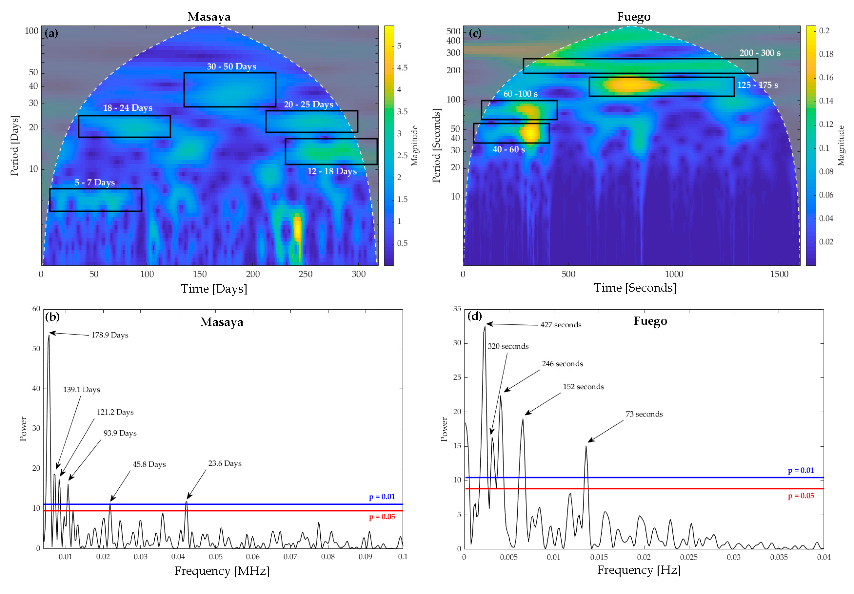
Fuego	Basalt	70–430 s	SO2 flux	[80], This Study
Gorely	Basalt	60–510 s	SO2 flux	[81], This Study
Kīlauea	Basalt	1–3600 s 1.6–7.8 h 4 m–15.8 h	Gas Pistoning; different ranges represent different time periods.	[82,83,84,85]
Llaima	Basalt	14 d	SO2 flux	[65]
Masaya	Basalt	200–300 s 50–180 d	SO2 flux	[17], This Study
Mayon	Andesite/Basaltic-Andesite	100–500 s 600–900 s 1200–1600 s 2000 s	H2O flux	[56]
Soufrière Hills	Andesite/Basaltic-Andesite	30–50 d 100–340 d	SO2 flux	[21,66]
Pacaya	Basalt	330–3000 s	SO2 flux	[86], This Study
Popocatépetl	Andesite/Basaltic-Andesite	250, 330 s	SO2 flux	[18]
Sabancaya	Andesite/Basaltic-Andesite/Dacite	240 s 120, 420 s	CO2/SO2 RatioSO2 flux	[26]
Stromboli	Basalt	~1–5 s 5–40 m	Strombolian activity	[87,88]
Turrialba	Andesite/Basaltic-Andesite	100 s 10–14 d	SO2 Flux	[89,90]
Ubinas	Andesite/Basaltic-Andesite	400–900 s 900–1200 s 1500–2500 s	SO2 Flux	[26], This Study
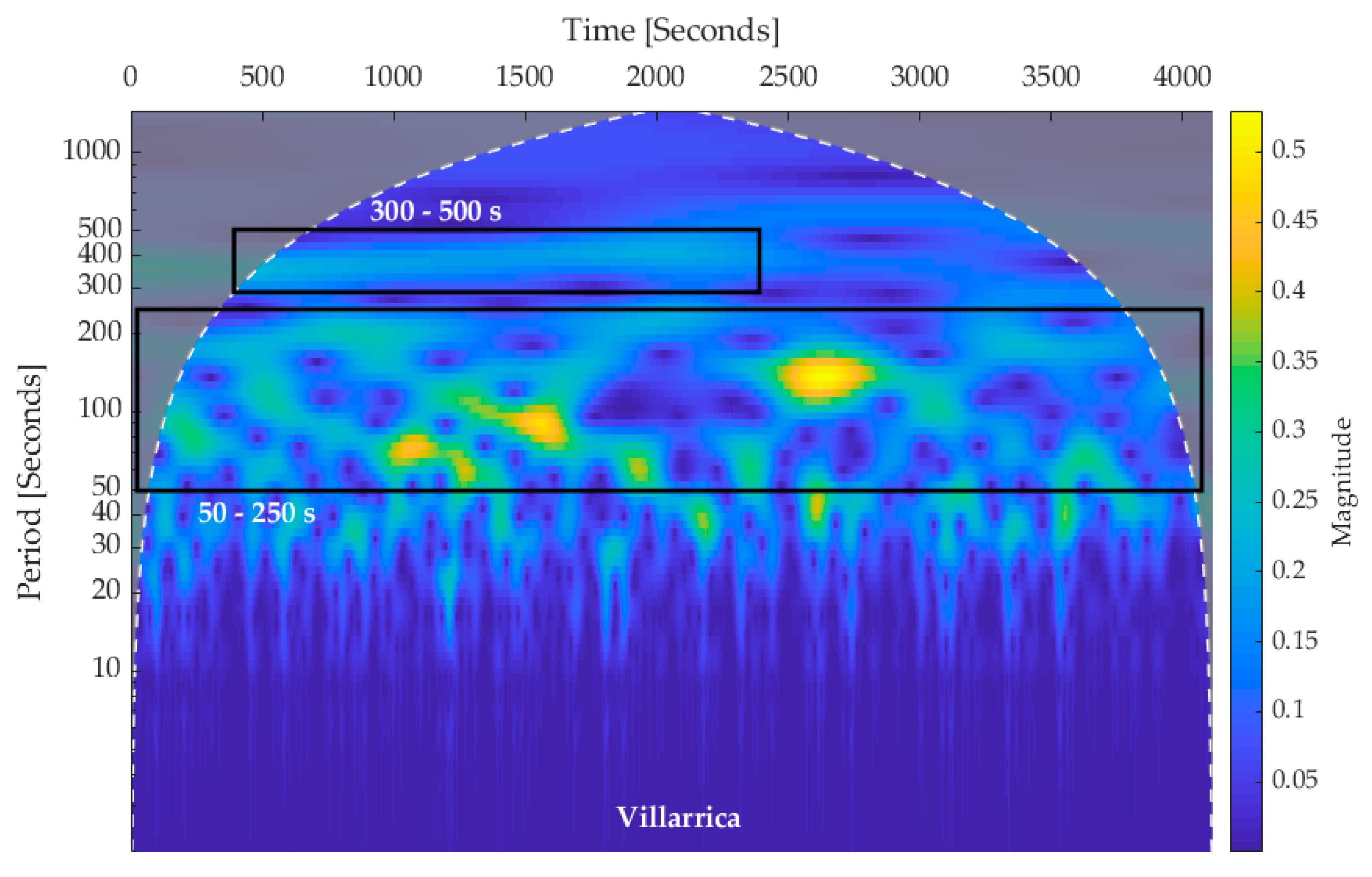
Villarrica	Basalt	None 30–50 s 340–710 s 14 d	SO2 flux SO2 concentration	[19,53,65]
Yasur	Basalt	~10 s–10 m	Strombolian activity	[29,91,92]

. In this section, we presented an overview of these studies and the interpretations made. We distinguished between studies that were based on single volatile species fluxes (commonly SO₂) and gas ratios (e.g., CO₂/SO₂). Furthermore, we highlighted several studies on volcanic plumes that have published flux or ratio timeseries at sufficient temporal resolution, but for which periodic degassing was not investigated. These data were extracted using an online data extraction tool, where required [74] (Available at: https://automeris.io/WebPlotDigitizer/) and reprocessed using the techniques described in Section 2. When using this tool, care was taken to extract data accurately and consistently. Although slight deviations (unfortunately unquantifiable) from the original data may have been introduced, the key focus of this study – periodicity – was not affected. Alternatively, in cases where data were provided as supplementary tables, these values were directly. Overview and analyses were split into three sections: (1) lava lakes; (2) basaltic volcanoes; (3) non-basaltic (andesite to rhyolite) volcanoes. These categorizations were selected based on the strong influence of magma rheology on in-conduit fluid dynamics, and thus bubble flow behaviour. Lava lakes, of all compositions, are dealt with separately due to their unique shallow geometry and our ability to directly observe the top of the magmatic column, which aids interpretation of degassing mechanisms.

3.1. Studies of Periodicity at Lava Lakes

Lava lakes are rare phenomena observed at only a handful of permanently open-vent volcanoes globally. Lakes manifest as a visible accumulation of magma at the top of the magma column, the longevity of which reflects a balance between surface cooling and heat supplied from beneath [93]. Recently active lava lakes include Nyiragongo (Democratic Republic of the Congo), Erta ‘Ale (Afar Depression, Ethiopia), Marum and Benbow (Ambrym, Vanuatu), Villarrica (Chile), Masaya (Nicaragua), Kilauea (Hawaii, USA), Mount Michael volcano (Saunders Island, South Sandwich Islands; [94]), and Erebus (Antarctica), although several have since subsided [93]. Given their persistent activity, lava lakes are prime ‘natural laboratories’ for the quantification of volcanic gas outgassing. Furthermore, the uninterrupted exposure of the magma surface at lava lake systems facilitates measurements of parameters absent at most closed system volcanoes, including surface velocity, heat flux, bubble burst frequency, crust coverage, and lake height. When combined with gas datasets, the independent constraints provided by these additional datasets aid the interpretation of the geophysical processes responsible for generating periodic degassing behavior at these volcanoes.

Benbow lava lake, Ambrym, is characterized by a turbulent over-turning lake surface and exhibits distinct periodicities in gas ratios on timescales of 100–200 s and 500 s [25]. These two cycles are attributed to the pulsation of gas bubbles in the upper portions of the conduit and to injections of gas-rich magma into the lava lake, respectively.

Gas emissions from the lava lake at Erebus were studied in detail [24,77,95]. This lake is unusual in that the dominant magma composition is phonolite and thus, characterized by far higher viscosities than other known lava lakes [96]. Ilanko et al. [24] highlighted a dominant periodicity of ~600 s in gas ratios and integrated column amounts (used as a proxy for gas flux) from OP-FTIR, building on previous observations of periods in SO₂ flux ranging from 240–900 s [76,95]. This timescale of periodicity is ascribed to the addition of magma into the shallow portions of the lake by pulses of lower viscosity magma in a bi-directional-flow, with pulses containing a higher proportion of exsolved gas [77,97]. This drives periodicity in degassing and other lake features such as plate movement and lake height [95,98]. Girona et al. [56] identified periodic components in SO₂ and H₂O flux, with the latter measured using visible imagery and plume pixel brightness as a proxy for water content. Here, FFT analysis identified ‘fractal degassing’, whereby H₂O emissions followed a well-defined fractal (power law) distribution across a wide range of frequencies (i.e., the timescale of periodicity decreased in tandem with increasing amplitude of the gas pulse). Interestingly, whilst two of the cycles identified at Erebus were shared by both H₂O and SO₂ (100–250 s and 500–650 s), a third was only manifest in SO₂ (300–450 s). The authors attribute the presence of decoupled cycles in multiple gas species to a thermochemical reaction, whereby exsolved bubbles from higher temperature magma batches contain elevated proportions of SO₂ compared to H₂O [30,56,99].

The Kīlauea’s Halema'uma'u crater hosted a lava lake from 2008 to 2018, with a surface behaviour that was similar (e.g., moving surface crustal plates) to Nyiragongo and Erta Ale. Distinct repeating co-variation in the gas (SO₂), thermal, and lake height measurements have been attributed to gas pistoning [82,83,84,85]. Gas pistoning is visually identified by a sustained rising of the lava level followed by a rapid drop, lasting a small fraction of the rise time, during this time SO₂ emissions are low prior to the rapid drop, increase rapidly on release of gas during the gas pistoning event and then return to normal [84]. Exact durations varied widely, from seconds to 15.8 hours, with the likely mechanism being the shallow accumulation of gas below the surface crust of the lake. The unique quality of the observations at Kīlauea are a direct result of the distinctly shallow generation mechanism, as modulations in degassing are frequently attributed to changes at deeper sources [85]. For example, at Erta ‘Ale, Bouche et al. [78] identified that large gas bubbles periodically broke the surface of the lake, in a similar location, suggesting that they have passed through the more constrained geometry of a feeding conduit.

The surface of the summit lava lake at Villarrica, Chile, is extremely turbulent, and initial investigations of outgassing based on crater rim gas measurements concluded that no periodicity could be detected [53]. The lack of periodic character was used to support a model of turbulent bi-directional magma mixing during ascent and descent within the conduit. However, a highly proximal gas timeseries collected using drone-based sampling demonstrated clearly-resolvable periodicities of 30–50 s (in all gas species), and highlighted that plume dilution and homogenization can be significant over length scales of <150 m [19]. Longer period cycles over at 345 to 714 were present in the SO₂ flux timeseries from a remote UV camera. Whilst the shorter-period cycles are temporally linked to discrete audible bubble bursts at the lake surface, the authors suggest that the longer-period cycles are atmospherically-generated through large-scale turbulent organization of the plume as it exits the crater [19]. Notably, in the original study Moussallam et al. [53] used autocorrelation, which, as we highlighted in Section 2, may not identify non-stationary periodic components. On extraction and reprocessing of data using Lomb-Scargle analysis, we also find no dominant periodicities, however, the CWT (Figure 3) shows a weakly stable period at ~300–500 s, which could be related to the 345–714 s period, identified by Liu et al. [19] in SO₂ flux data and could also be caused by atmospheric transport phenomena.

Aiuppa et al. [35] published long-term gas monitoring data at Masaya highlighting an increase CO₂/SO₂ ratio prior to the onset of lava lake activity. Here, we used their NOVAC (Network for Observation of Volcanic and Atmospheric Change) data, which spans over the period March 2014 to September 2016 [100], and conducted CWT and Lomb-Scargle analysis to highlight the presence of significant periodic components within the SO₂ flux dataset (Figure 4a,b). In the Lomb-Scargle analysis (Figure 4b), the dominant of these has a period of 178.9 days, which we noted is similar to the duration of the solar semiannual tide at 182.6 days (the semiannual tide) [101]. Another cycle has a 23.6 day period, which appears too short to be linked to the lunar 27.6 day cycle [27,101]. Further periodicities at 140, 121, 94, and 46 days could reflect the volcanic influence at Masaya, involving replenishment of magma into storage zones, necessary to feed the observed high degassing rates of Masaya [35,102] which will also reflect changes in surface behaviour of the lava lake [17,93]. Given the large dataset gaps, it was only possible to conduct the CWT over a portion of the dataset between 16/11/2015 and 30/09/2016. The CWT (Figure 4a) shows multiple periodicities (5–7, 12–18, 18–24, 20–25, and 30–50 days) which overlap with Lomb-Scargle values (24 and 36 days) but with none that are present for the entire dataset, which would appear to rule out a dominant effect of tidal forcing, at least over timescales < 50 days. Co-acquired timeseries of SO₂ flux, thermal and visible video imagery of the Masaya lava lake over sampling windows of seconds to hours, revealed a periodic component of ~200–300 s in the SO₂ flux data, attributed to atmospheric processes given a lack of cyclic behaviour in the other co-acquired datasets [17].

3.2. Studies of Periodicity at Basaltic Volcanoes

Etna, Italy, is one of the best characterized of all basaltic volcanoes in terms of volcanic gas emissions. Using a UV camera, Tamburello et al. [15] identified two sets of periodicities in a high resolution SO₂ flux timeseries: short-period cycles of 40–250 s (centred on 150 s), and long-period cycles of 500–1200 s (centred on 600 s). The higher frequency periodicities were often sustained on timescales of tens of minutes. Similarly, Pering et al. [16] also identified short-period cycles of ~89 and ~185 s in SO₂ flux, but also identified a mid-range period of ~340 s. Importantly, the ~89 s cycle was also observed in the CO₂/SO₂ molar ratio (measured using an independent MultiGAS analyser), and therefore, could not be driven by atmospheric processes. Specifically, no plausible mechanism exists for fractionating one gas species from another preferentially during plume transport on the length scales analysed. Finally, Pering et al. [79] identified a similar range of short-period oscillations in SO₂, CO₂, and H₂O flux of ~40–175 s cycles. Intriguingly, the authors discovered stronger links between degassing of SO₂ and H₂O than for CO₂ with each of these, suggesting that a shared periodicity could be due to similar exsolution depth [103,104] and process operating across this length-scale. Indeed, given that stronger links were found between H₂O and SO₂ than CO₂ this would suggest a volcanogenic cause, otherwise periodicity would be shared between all three species. Waves of bubbles [105] ascending and bursting at the summit were suggested as a cause by Tamburello et al. [15], whereby bubbles self-organize into layers observed as periodicity at the surface. The detection of longer period components at Etna is often limited by total measurement duration for high-resolution acquisitions.

Degassing at Stromboli, Italy, is dominated by impulsive gas slug-driven explosions, which occur on the order of minutes from the multiple vents active in the summit area [87]. Similarly, degassing at Yasur (Vanuatu) is also dominated by impulsive slug-driven explosions [29,91,92]. The explosive activity forms an important part of the degassing record and the resultant frequency characteristics at these volcanoes. Indeed, patterns in explosive events could be linked to the fluid dynamics of the bubbles which drive them [106,107,108]. Spampinato et al. [88] highlight the periodic characteristics of explosive activity on Stromboli and Etna in thermal data (which would also manifest as changes in degassing). At Etna the authors highlight distinct periods of 4–9 s, 23–45 s, and 1–10 min. The shortest timescale is attributed to puffing, i.e., the bursting of larger non-pressurized bubbles [107,108] while the latter timescales are associated with clusters of bubbles (or slug trains, see Pering et al. [109]) arriving periodically at the surface. Of particular interest is the matching of these to phases in activity, whereby longer periods of 1–10 min are associated with stronger gas supply [88]. At Stromboli, Ripepe et al. [87] and Spampinato et al. [88] focused on puffing activity showing a change in the vigor of activity, 1–2 s and 3–5 s during stronger and weaker phases respectively, with this activity occurring over periods of 5–8 and 5–40 min cycles, likely associated with overall gas supply from depth. Any consideration of periodic components in long-term passive gas flux on the order of seconds to hours would require deconvolution from the active degassing (i.e., the explosive strombolian eruptions or puffing).

At Fuego (Guatemala), Nadeau et al. [80] highlighted the presence of a correlation between SO₂ and seismicity, however, they did not comment on the presence of shorter-period cycles, which are visible (by eye) in Figure 2c. By extracting this data and using Lomb-Scargle analysis, we indeed highlighted a dominant periodic component of 427 s, with others ranging from 73 to 320 s (see Figure 4d). The CWT (Figure 4c) also highlights stable periods of 200–300 s and 125–175 s. It is plausible that these periodic components are related to the rheological stiffening of the upper conduit, which was posited by Nadeau et al. [80] as a cause of the link between seismicity and gas release. Similarly, reanalysis of timeseries data from Gorely [81] and Pacaya, Guatemala [86] revealed a range of periodicities. At Gorely, a dominant period was discovered at 63 s, with others at 197 and 509 s in Lomb-Scargle analysis (Figure 5b), while the CWT (Figure 5a) shows a period of 350-600 s and 150–250 s which highlights overlap, a further area at 50–120 s was related to transient events in the flux record. At Pacaya, a broad range of 331–3000 s appeared in Lomb-Scargle analysis (Figure 5d), with dominant periods at 3000 s and 1920 s, and less prominent at 1143 s, 353 s, and 331 s. The CWT (Figure 5c) shows that some of these are present for a large proportion of the dataset (900–1400 s and 1500–2500 s) but that spikes between 200–700 s were more transient and likely related to the mild strombolian activity during acquisition [86].

3.3. Studies of Periodicity at Predominantly Non-Basaltic Volcanoes

Recently published data for Peruvian volcanoes highlight periodicity at Sabancaya, a basaltic-andesite to dacite volcano, of ~240 s in CO₂/SO₂ ratio data and of ~120 s and ~420 s from UV camera SO₂ flux data, noting that these two timeseries were not contemporaneous [26]. These measurements were made during a phase of relative eruptive quiescence characterized by continuous passive degassing. The authors noted that such a short-period cycles are unusual for a volcano with a higher viscosity magma. The authors invoked a shallow conduit process involving convection of a gas-rich magma to explain this cyclicity. At Ubinas, Moussallam et al. [26] noted no quantifiable periodicity but did describe ‘puffing’ style activity, where clearly defined gas pulses were released from the summit (similar to observations of Masaya in Pering et al. [17] and Villarrica in Liu et al. [19]). Here, using Lomb-Scargle analyses on extracted data, no significant periods were discovered, although CWT analysis (Figure 6) suggested possible longer term periods between 400–900 s and 900–1200 s which are potentially related to puffing behavior observed by the authors at the time [26].

Popocatépetl (Mexico), which has a lava dome of andesitic/basaltic-andesite emplaced at the summit, is a prolific emitter of SO₂ on a global scale. Campion et al. [18] discovered distinct periodic components in passive degassing at ~300 s (252 and 328 s), and argued that the thermal buoyancy of the hotter gas released from the vents and the regularity of release mean that the most plausible mechanism was a volcanic origin. Although they did not explicitly ascribe a causal mechanism, Campion et al. [18] did suggest that gas puffing and explosions could be driven by closure of vesicle networks in the melt, which are responsible for high rates of passive degassing. Smaller changes in gas flux through vesicle networks could also be the driver of short-period cycles in passive degassing, and could be a common process at volcanoes with a lava dome or for volcanoes with more evolved magmas, e.g., a ~100-s period was also found in gas flux at Turrialba (Costa Rica) [18,89].

Eruptive activity at Soufrière Hills volcano (Montserrat) is characterized by repeated growth and collapse of an andesitic/basaltic-andesite lava dome, and has been in eruption since 1995. The installation of a long-term SO₂ flux monitoring network has generated a multi-decadal timeseries (2002-present) that is unprecedented in its completeness, thus enabling investigation of periodicity on longer timescales than usual possible in emissions datasets [21,23,110]. Analysing daily flux averages from the interval 2002–2011 (spanning 4 eruptive phases and pauses), revealed dominant cycles evident on both multi-year and multi-week (~50 day) timescales. The short-term cycles persisted through phases of both active extrusion and eruptive pause and broadly correlated to enhanced lava extrusion and elevated seismicity. However, phase offsets of ~4 days were found between the onset of each initial low-frequency seismic pulse and peaks in SO₂ flux [21]. Interestingly, the strength of the multi-week cycle appeared to be strongly influenced by the occurrence of explosive activity, being manifest most strongly in the lead-up to such an event; the authors therefore suggested that the amplitude of surface gas flux cycles is modulated by physical conditions within the conduit, a conclusion supported by conduit models [111]. In contrast, the long-term multi-year cycle in SO₂ flux is decoupled from magma extrusion and other geophysical parameters [112]. Flower and Carn [66] also highlighted the utility of using satellite thermal and SO₂ measurements, identifying longer period cycles of 102, 121, and 159 days which were posited to relate to magma intrusion, whilst a longer period of 238 days was associated with lava dome destabilization.

At Mayon (Phillipines), which erupts andesitic/basaltic-andesitic magma and is characterized by persistent passive degassing, Girona et al. [56], identified four discrete timescales of periodicities in H₂O flux data, with the following periods: ~100–500 s (intermittent in strength and duration throughout acquisition), ~600–900 s (stable), ~1200–1600 s (stable), and 2000 s (but just within the detection limit using a CWT). The authors did not posit a causal mechanism, specific to this volcano, although the range of periodicities, the timescales they operate over, and the similarity to those at other volcanoes of similar composition suggests that the drivers may be volcanogenic, particularly for the longer periodicities > 600 s.

Dinger et al. [27] identified a period of 13.7 days in BrO/SO₂ ratios using DOAS (daily averages over a three month dataset) at Cotopaxi (an andesitic/basaltic-andesitic volcano), which they attributed to a fortnightly lunar tidal force, with correlation coefficients of 0.47 and 0.36 (representing links with the North-South and vertical tidal displacements respectively). It is important to note here that the presence of a correlation does not imply causation. The data from Figure 6 in Dinger et al. [27] were extracted and reprocessed, first using Pearson’s correlation to check for matching correlation coefficient of 0.47 and then further processed using regression (conducted in SPSS). The correlations listed in Dinger at al. [27] therefore equate to regression coefficients of 22% (R² = 0.22, see Figure 7) and 13% (R² = 0.13) respectively. It is this regression coefficient that we can use to model the change in one variable (the BrO/SO₂ ratio) that can be accounted for by another (the tide). The relationship is highlighted in Figure 7 alongside residuals to the linear fit, showing variability. The exact p-value for the 22% regression coefficient is below the p < 0.01 significance level at p = 2.5 × 10⁻⁵. Whilst the North-South tide has a statistically significant relationship with BrO/SO₂ there is still a large proportion of unexplained variability; indeed, 78% of the signal can be attributed to other factors (i.e., random fluctuations, error, or a volcanogenic component). The detection of periodicity in BrO/SO₂ could reflect a complex process whereby tides preferentially effect degassing of one species relative the other, related to differences in solubility and points of saturation in the melt.

Other studies have also hypothesized tidal influences on degassing at Villarrica and Llaima, Chile, where there also appeared to be a shared period component in SO₂ flux driven by a fortnightly lunar tide, with low correlation coefficients of 0.2–0.3 [65], which give R² values of 0.04–0.09 (4–9%), hence presenting a weak relationship. Turrialba, also exhibited a 10–14 day period in SO₂ flux, which could be tidally induced [90]. Finally, the periods that can be detected are limited by sampling duration and frequency, and this must be considered during data collection if investigation of longer or shorter periodicities is planned.

4. Comparison of Volcanoes and Potential Drivers of Periodicity

This review summarized the literature to date discussing periodicity in gas flux and ratios. Many volcanoes, spanning different tectonic settings and magma compositions, display periodic degassing with cycle durations of seconds to months. Here, we attempted to synthesize the causal mechanisms invoked in the various studies presented into a general framework that accounts for the different timescales of periodic behaviour identified. This framework includes the following categories, in order of increasing timescale: (C1) atmospheric and non-volcanic generation; (C2) gas-driven shallow processes, such as discrete bubble bursts and waves of bubbles; (C3) shallow magma movement in a conduit or shallow storage zone; or (C4) deep magmatic processes. These are summarized in

Table 3. A summary of the main drivers of periodic degassing at volcanoes.

Category	Description	Dominant Range
C1	Non-volcanic, atmospheric- or tidal- generated	Variable
C2	Gas-driven, shallow process	Seconds to Hours
C3	Shallow magma movement, in-conduit or shallow storage	Minutes to Days
C4	Deep magmatic processes	Days to Months

, along with suggested timescales for such processes.

4.1. Non-Volcanic Periodicity (C1)

The height and relief of many volcanoes, and particularly the presence of large topographic features such as calderas, contribute to unique microclimatic conditions that can generate apparent periodicity. By perturbing local wind fields, topographically-induced eddying, dispersion and large-scale organization of turbulence can result in rhythmic fluctuations in gas concentration and/or flux [15,76]. Crucially, though, if a periodicity is detected within a proximal timeseries of gas molar ratios, then this can only be reliably explained by primary magmatic processes, e.g., [16]. Once outgassed to the atmosphere, all gas species will be subject to similar meteorological processes, and from measurement positions close to the vent, little conversion of SO₂ would occur through photochemical reactions. Moreover, atmospherically-driven periodicities are likely to operate towards the high frequency end of the spectrum, on timescales of tens of seconds to minutes. Over minutes, topographic features, such as a caldera or an elevated crater, could facilitate the buildup and periodic release of gases as a result of local pressure differences and wind-fields, e.g., [113], and is probably the case with the 200–300 s periodicity at Masaya [17].

An additional non-volcanic mechanism is tidal forcing. There is some evidence for the presence of 14 day cycles at four volcanoes: Villarrica and Llaima [65], Turrialba [90], and Cotopaxi [27]. Dinger et al. [114] developed a model suggesting that tidal forcing could affect the rate of bubble coalescence in the conduit, which is then manifested as change in degassing behavior measured at the surface. Overall, for volcano monitoring, deconvolving tidal influences from volcanically generated signals is crucial to the isolation of changes in the degassing regime.

4.2. Periodicities Generated within the Shallow Plumbing System (C2 and C3)

The differing fluid dynamic regimes in volcanic conduits are complex, and therefore, can modulate volcanic outgassing in a periodic manner. The main controls on volatile (bubble) flow behaviour, and hence on gas-driven periodicity (C2), are: magma rheology (density, viscosity and crystal content, which influence permeability and gas-melt separation), conduit diameter, total gas volume, depth (and hence pressure), bubble morphology, and magma convection [16,115,116].

In low viscosity, low crystallinity magmas that approximate near-Newtonian behaviour (predominantly basalts), bubbles are able to decouple from the melt, move freely and coalesce. In this way, waves of bubbles can develop via self-organization [105]. Where larger coalesced bubbles are involved, e.g., spherical-cap bubbles and Taylor bubbles (gas slugs), their periodic eruptive release lead to distinct, impulsive and short-lived peaks in flux records. In low viscosity systems, it is therefore the dynamics of bubble formation and ascent that generates periodicity. For example, the accumulation of gas at a geometrical or rheological discontinuity in the conduit or shallow storage zone; the coalescence of bubbles during decoupled ascent through the melt [2,16,117]. The timescales of these processes are directly related to visible explosion events at the surface, which at Stromboli could be on the order of 5–10 min [87] or, at a volcano such as Yasur, tens of seconds [92]. Similarly, ‘puffing’ represents a non-explosive manifestation of periodic impulsive gas release during puffing events, which are likewise evident at Stromboli [108]. An alternative mechanism, gas pistoning, describes the viscoelastic response of the surface of a magma column to accumulating bubbles beneath a crust [82]. Pistoning has been observed at Kilauea, Hawaii [85] but intriguingly, despite similar lake surface characteristics, this was not posited as the cause of lake fluctuations at Nyiragongo, Democratic Republic of the Congo, another basaltic lava lake, which were attributed to deeper sources [118]. The process operates over a large range of timescales (seconds to hours), and is preferentially manifest at more stable lava lakes; i.e., those with a surface crust, in contrast to the more turbulent surfaces at Ambrym, Masaya or Villarrica, Chile. It is possible, therefore, that such a mechanism may also operate at non-lava lake volcanoes where the surface of the magma column is out if sight.

By contrast, in high viscosity non-Newtonian magmas, networks of bubbles can facilitate the permeable movement of gas through a magma, and the periodic opening and closing of such networks may induce periodicity [18,119]. In these systems, the crystal content (and shape [120]) strongly modifies the free permeability and the ease by which volatiles can be outgassed [121].

In-conduit processes could also be linked to magma movement (C3) as well as to a discrete gas phase; for example, the periodic rise of gas-rich magma batches (or pulses) is a mechanism invoked at Erebus [77]. In-conduit convection can disrupt or enable periodicity. Where magma ascent may be turbulent, e.g., at lava lakes such as Villarrica, Ambrym, and Masaya any organization of bubbles would be disrupted within a turbulent magma column [53]. However, where convection is more stable, periodicity may be encouraged, or even driven by, the form of convection. Cycles in gas ratios at Erebus have been traced both to gas-phase redox reactions (affecting species such as CO, CO₂, OCS, and potentially SO₂) and to shallow exsolution of more soluble species (H₂O, SO₂, HCl, and HF) from fresh magma input to the lava lake [24].

4.3. Periodicity in Magma Storage Region (C4)

Longer term variations in gas release over days to months (and years where datasets are available) can be broadly attributed to processes occurring deeper in the magmatic system, such as (a) the addition of new hot, volatile-rich magma to a storage zone and the rejuvenation of the resident magma body, or (b) deep volatile segregation, leading to recurring mush destabilization and upwards melt-decoupled volatile transport [110,112,122]. These processes are considered exemplified at Soufriere Hills Volcano, Montserrat, a long-lived, vertically-extensive transcrustal mush system. Long-term magma input and volatile segregation produces broad cycles in SO₂ flux (and other geophysical parameters [51]) over timescales of 2–3 years, on which short-term shallow gas periodicities are superposed [21,66,110]. Crucially, these long-term gas cycles are decoupled from phases of magma extrusion or variations in other geophysical parameters, indicating that the underlying periodicity-generating mechanism is intrinsically related to the timescales of volatile-melt separation [112]. In silicic systems, SO₂ flux can be used as a first-order indicator of the efficiency and rate of mafic injection at depth [110].

Although beyond the scope of this review, we highlight that periodicity in volcanic gas emissions can also be manifest in timeseries of regional diffuse degassing. Berberich et al. [123] identified periodic fluctuations in degassing from mineral springs in the East Eifel Volcanic Field, Germany, on timescales of 1 day (solar diurnal cycle), 4–6 days and 10–15 days, which they suggested reflected either variations in the deep gas source, changes in the transport pathway for gases to reach the surface, or the influence of volcano-tectonic earthquakes. Soil degassing (predominantly CO₂) can also provide good indications of the onset of volcanic unrest and magma movement at depth [124], although such datasets can also be sensitive to environmental and climatic influences [125,126]; for example, 47% of the soil CO₂ flux variations at Fogo, Azores, could be explained by the effect of the soil and air temperature, wind speed, and soil water content [127].

4.4. Synthesis

In summary, detected periodicities span a large range, from seconds through to hundreds of days. The timescale of periodicity is likely intrinsically linked to source process, which is clearer for some periodic driving mechanisms than for others. Perhaps the least is known about causal drivers of periodicities of tens of seconds to minutes, and specifically whether they may be atmospherically generated or driven by in-conduit processes, such as convection or gas pistoning. It is clear that the most detailed information elucidating drivers of periodic degassing come from multiparametric studies, i.e., those involving measurements of multiple gas species or in combination with other geophysical datasets, for example, where periodic components are shared, or not, between contemporaneous flux or ratio measurements [16,56,79], or where measurements of processes occurring directly at the magma surface corroborate via audible bubble bursts [19] or do not corroborate periodicity [17]. Of particular importance is when gas periodicities are also reflected in seismic and deformation datasets, e.g., as at Soufriere Hills [21,23].

To some extent, our assessment of periodic components within degassing datasets is significantly limited, and in some cases, biased by the choice of technique: namely, temporal resolution, and the length of continuous timeseries. Installation of permanent DOAS networks for SO₂ flux, such as those of NOVAC [100] are optimized to study cycles with periods of hours to days in SO₂ flux, given that scanning can take tens of minutes to complete. Meanwhile, high sampling rate techniques, such as the UV camera, are capable of robustly identifying high frequency periodic components, yet long datasets spanning longer than several hours are rare and limited to permanent networks (e.g., Stromboli [128]; and Etna, [129]). The need to regularly recalibrate the UV camera during campaign field acquisitions (i.e., when using SO₂ gas cells) also introduces data gaps, thus precluding the detection of periodic components longer than a calibration window within collected datasets [130]. Similarly, high time resolution measurements of gas composition using MultiGAS or Fourier Transform Infrared (FTIR) instruments are often limited to discrete sampling intervals during field campaigns. Although, there are currently ~25 permanent MultiGAS installations on active volcanoes worldwide, they often only acquire for 4 × 1 h measurement windows each day, thus precluding the detection of intermediate cyclicity on a scale of hours [131]. Finally, it may be possible to improve our long term datasets through the use of satellite observations and methods, which can derive high time resolution SO₂ flux measurements, for example, using the method of Queißer et al. [132] or as demonstrated by Flower and Carn [66] for Soufrière Hills Volcano. Spatially, mixing and homogenization of volcanic plumes can occur rapidly on horizontal length scales of <150 m, with varying timescales of periodicity evident at different distances of observation, or obscured, e.g., Liu et al. [19]. The measurement technique, and region of plume targeted, should always be taken into account when directly comparing periodic characteristics between timeseries.

4.5. Future Challenges in Periodicity Analysis

From this synthesis, we propose that the following outstanding questions be targeted in future studies of periodicity in volcanic gas emissions:

• What are the dominant controls on long-term stability of short-duration periodicity (< an hour)?
• Is there a relationship between total emission fluxes and either the magnitude or timescale of periodicity? If so, how can this help inform our understanding of subsurface processes?
• How do the properties of periodic behaviour change in the time before/after eruptive events, and can these be used to aid in hazard assessment and eruption forecasting?
• Do tidal forces have an effect on volcanoes and, if so, what is the magnitude of oscillation compared to volcanogenic mechanisms? What other external forcings should be considered?
• At multi-vent volcanoes, do the periodic characteristics of outgassing vary between craters? If so, what can this tell us about shallow subsurface plumbing systems?
• Do phase offsets exist between emissions of different gas species, i.e., highlighting a specific source depth for periodicity?

5. Conclusions

This review highlighted the range of studies to discover and highlight periodic components within volcanic degassing datasets, revealing these to be commonplace among a suite of volcanoes with different characteristics globally. Furthermore, we included the best techniques for investigating periodicity. At this stage, more work needs to be done on the driving mechanisms for short term periodic components and what they may tell us about the dynamics of gas release from magmas. Overall, we detail four main categories of periodic degassing: C1—non-volcanic; C2—gas-drive shallow process; C3—shallow magma movement in-conduit or shallow storage zone; and C4—deep magmatic processes.

Periodic behavior in volcanic emissions is fundamentally related to the physical processes controlling gas exsolution, migration, and outgassing, processes which also modulate eruptive activity and, specifically, transitions between phases of passive degassing and explosive activity. We highlight the importance of visible and audible observations of the magma surface to aid interpretation of geophysical and geochemical measurements. A more holistic understanding of the mechanisms generating different timescales of periodicity in volcanic gas emissions will improve our ability to utilize gas monitoring for volcanic hazard assessment at volcanoes in different tectonic settings.

References

- Shaw, H.R.; Wright, T.L.; Peck, D.L.; Okamura, R. The viscosity of basaltic magma; an analysis of field measurements in Makaopuhi lava lake, Hawaii. Am. J. Sci. 1968, 266, 225–264. [Google Scholar] [CrossRef]
- Parfitt, E.A. A discussion of the mechanisms of explosive basaltic eruptions. J. Volcanol. Geotherm. Res. 2004, 134, 77–107. [Google Scholar] [CrossRef]
- Sparks, R.S.J. The dynamics of bubble formation and growth in magmas: A review and analysis. J. Volcanol. Geotherm. Res. 1978, 3, 1–37. [Google Scholar] [CrossRef]
- Namiki, A.; Manga, M. Transition between fragmentation and permeable outgassing of low viscosity magmas. J. Volcanol. Geotherm. Res. 2008, 169, 48–60. [Google Scholar] [CrossRef]
- Cashman, K.V.; Scheu, B. Magmatic Fragmentation. Encycl. Volcanoes 2015, 459–471. [Google Scholar]
- McGonigle, A.J.S.; Pering, T.D.; Wilkes, T.C.; Tamburello, G.; D’Aleo, R.; Bitetto, M.; Aiuppa, A.; Willmott, J.R. Ultraviolet Imaging of Volcanic Plumes: A New Paradigm in Volcanology. Geosciences 2017, 7, 68. [Google Scholar] [CrossRef]
- Oppenheimer, C.; Tsanev, V.I.; Braban, C.F.; Cox, R.A.; Adams, J.W.; Aiuppa, A.; Bobrowski, N.; Delmelle, P.; Barclay, J.; McGonigle, A.J.S.S. BrO formation in volcanic plumes. Geochim. Cosmochim. Acta 2006, 70, 2935–2941. [Google Scholar] [CrossRef]
- Schönhardt, A.; Richter, A.; Theys, N.; Burrows, J.P. Space-based observation of volcanic iodine monoxide. Atmos. Chem. Phys 2017, 17, 4857–4870. [Google Scholar] [CrossRef]
- Gutmann, A.; Bobrowski, N.; Roberts, T.J.; Rüdiger, J.; Hoffmann, T. Advances in Bromine Speciation in Volcanic Plumes. Front. Earth Sci. 2018, 6, 213. [Google Scholar] [CrossRef]
- Mori, T.; Burton, M. The SO2 camera: A simple, fast and cheap method for ground-based imaging of SO2 in volcanic plumes. Geophys. Res. Lett. 2006, 33, L24804. [Google Scholar] [CrossRef]
- Bluth, G.J.S.; Shannon, J.M.; Watson, I.M.; Prata, A.J.; Realmuto, V.J. Development of an ultra-violet digital camera for volcanic SO2 imaging. J. Volcanol. Geotherm. Res. 2007, 161, 47–56. [Google Scholar] [CrossRef]
- McGonigle, A.J.S.; Oppenheimer, C.; Galle, B.; Mather, T.A.; Pyle, D.M. Walking traverse and scanning DOAS measurements of volcanic gas emission rates. Geophys. Res. Lett. 2002, 29, 1–4. [Google Scholar] [CrossRef]
- Galle, B.; Oppenheimer, C.; Geyer, A.; McGonigle, A.J.; Edmonds, M.; Horrocks, L. A miniaturised ultraviolet spectrometer for remote sensing of SO2 fluxes: A new tool for volcano surveillance. J. Volcanol. Geotherm. Res. 2003, 119, 241–254. [Google Scholar] [CrossRef]
- Kantzas, E.P.; McGonigle, A.J.S. Ground Based Ultraviolet Remote Sensing of Volcanic Gas Plumes. Sensors 2008, 8, 1559–1574. [Google Scholar] [CrossRef]
- Tamburello, G.; Aiuppa, A.; McGonigle, A.J.S.; Allard, P.; Cannata, A.; Giudice, G.; Kantzas, E.P.; Pering, T.D. Periodic volcanic degassing behavior: The Mount Etna example. Geophys. Res. Lett. 2013, 40, 4818–4822. [Google Scholar] [CrossRef]
- Pering, T.D.; Tamburello, G.; McGonigle, A.J.S.; Aiuppa, A.; Cannata, A.; Giudice, G.; Patanè, D. High time resolution fluctuations in volcanic carbon dioxide degassing from Mount Etna. J. Volcanol. Geotherm. Res. 2014, 270, 115–121. [Google Scholar] [CrossRef]
- Pering, T.D.; Ilanko, T.; Wilkes, T.C.; England, R.A.; Silcock, S.R.; Stanger, L.R.; Willmott, J.R.; Bryant, R.G.; McGonigle, A.J.S. A Rapidly Convecting Lava Lake at Masaya Volcano, Nicaragua. Front. Earth Sci. 2019, 6, 241. [Google Scholar] [CrossRef]
- Campion, R.; Delgado-Granados, H.; Legrand, D.; Taquet, N.; Boulesteix, T.; Pedraza-Espitía, S.; Lecocq, T. Breathing and Coughing: The Extraordinarily High Degassing of Popocatépetl Volcano Investigated With an SO2 Camera. Front. Earth Sci. 2018, 6, 163. [Google Scholar] [CrossRef]
- Liu, E.J.; Wood, K.; Mason, E.; Edmonds, M.; Aiuppa, A.; Giudice, G.; Bitetto, M.; Francofonte, V.; Burrow, S.; Richardson, T.; et al. Dynamics of Outgassing and Plume Transport Revealed by Proximal Unmanned Aerial System (UAS) Measurements at Volcán Villarrica, Chile. Geochem. Geophys. Geosystems 2019, 20, 730–750. [Google Scholar] [CrossRef]
- Connor, C.B.; Stoiber, R.E.; Malinconico, L.L. Variation in sulfur dioxide emissions related to earth tides, Halemaumau Crater, Kilauea Volcano, Hawaii. J. Geophys. Res. Solid Earth 1988, 93, 14867–14871. [Google Scholar] [CrossRef]
- Nicholson, E.J.; Mather, T.A.; Pyle, D.M.; Odbert, H.M.; Christopher, T. Cyclical patterns in volcanic degassing revealed by SO2 flux timeseries analysis: An application to Soufrière Hills Volcano, Montserrat. Earth Planet. Sci. Lett. 2013, 375, 209–221. [Google Scholar] [CrossRef]
- Rymer, H.; Locke, C.A.; Brenes, J.; Williams-Jones, G. Magma plumbing processes for persistent activity at Poás volcano, Costa Rica. Geophys. Res. Lett. 2005, 32, L08307. [Google Scholar] [CrossRef]
- Christopher, T.; Edmonds, M.; Taisne, B.; Odbert, H.; Costa, A.; Hards, V.; Wadge, G. Periodic sulphur dioxide degassing from the Soufrière Hills Volcano related to deep magma supply. Geol. Soc. Lond. Spec. Publ. 2015, 410, 123–141. [Google Scholar] [CrossRef]
- Ilanko, T.; Oppenheimer, C.; Burgisser, A.; Kyle, P. Cyclic degassing of Erebus volcano, Antarctica. Bull. Volcanol. 2015, 77, 56. [Google Scholar] [CrossRef]
- Allard, P.; Burton, M.; Sawyer, G.; Bani, P. Degassing dynamics of basaltic lava lake at a top-ranking volatile emitter: Ambrym volcano, Vanuatu arc. Earth Planet. Sci. Lett. 2016, 448, 69–80. [Google Scholar] [CrossRef]
- Moussallam, Y.; Tamburello, G.; Peters, N.; Apaza, F.; Schipper, C.I.; Curtis, A.; Aiuppa, A.; Masias, P.; Boichu, M.; Bauduin, S.; et al. Volcanic gas emissions and degassing dynamics at Ubinas and Sabancaya volcanoes; implications for the volatile budget of the central volcanic zone. J. Volcanol. Geotherm. Res. 2017, 343, 181–191. [Google Scholar] [CrossRef]
- Dinger, F.; Bobrowski, N.; Warnach, S.; Bredemeyer, S.; Hidalgo, S.; Arellano, S.; Galle, B.; Platt, U.; Wagner, T. Periodicity in the BrO/SO2 molar ratios in the volcanic gas plume of Cotopaxi and its correlation with the Earth tides during the eruption in 2015. Solid Earth 2018, 9, 247–266. [Google Scholar] [CrossRef]
- Oppenheimer, C.; Francis, P.; Burton, M.; Maciejewski, A.J.H.; Boardman, L. Remote measurement of volcanic gases by Fourier transform infrared spectroscopy. Appl. Phys. B Lasers Opt. 1998, 67, 505–515. [Google Scholar] [CrossRef]
- Oppenheimer, C.; Bani, P.; Calkins, J.A.; Burton, M.R.; Sawyer, G.M. Rapid FTIR sensing of volcanic gases released by Strombolian explosions at Yasur volcano, Vanuatu. Appl. Phys. B 2006, 85, 453–460. [Google Scholar] [CrossRef]
- Oppenheimer, C.; Kyle, P.R. Probing the magma plumbing of Erebus volcano, Antarctica, by open-path FTIR spectroscopy of gas emissions. J. Volcanol. Geotherm. Res. 2008, 177, 743–754. [Google Scholar] [CrossRef]
- Burton, M.; Allard, P.; Mure, F.; La Spina, A. Magmatic Gas Composition Reveals the Source Depth of Slug-Driven Strombolian Explosive Activity. Science 2007, 317, 227–230. [Google Scholar] [CrossRef]
- La Spina, A.; Burton, M.; Allard, P.; Alparone, S.; Muré, F. Open-path FTIR spectroscopy of magma degassing processes during eight lava fountains on Mount Etna. Earth Planet. Sci. Lett. 2015, 413, 123–134. [Google Scholar] [CrossRef]
- Aiuppa, A.; Moretti, R.; Federico, C.; Giudice, G.; Gurrieri, S.; Liuzzo, M.; Papale, P.; Shinohara, H.; Valenza, M. Forecasting Etna eruptions by real-time observation of volcanic gas composition. Geology 2007, 35, 1115. [Google Scholar] [CrossRef]
- Aiuppa, A.; Federico, C.; Giudice, G.; Giuffrida, G.; Guida, R.; Gurrieri, S.; Liuzzo, M.; Moretti, R.; Papale, P. The 2007 eruption of Stromboli volcano: Insights from real-time measurement of the volcanic gas plume CO2/SO2 ratio. J. Volcanol. Geotherm. Res. 2009, 182, 221–230. [Google Scholar] [CrossRef]
- Aiuppa, A.; de Moor, J.M.; Arellano, S.; Coppola, D.; Francofonte, V.; Galle, B.; Giudice, G.; Liuzzo, M.; Mendoza, E.; Saballos, A.; et al. Tracking Formation of a Lava Lake From Ground and Space: Masaya Volcano (Nicaragua), 2014–2017. Geochem. Geophys. Geosystems 2018, 19, 496–515. [Google Scholar] [CrossRef]
- Edmonds, M. New geochemical insights into volcanic degassing. Philos. Trans. R. Soc. A Math. Phys. Eng. Sci. 2008, 366, 4559–4579. [Google Scholar] [CrossRef]
- Burgisser, A.; Scaillet, B. Redox evolution of a degassing magma rising to the surface. Nature 2007, 445, 194–197. [Google Scholar] [CrossRef]
- Cochran, W.T.; Cooley, J.W.; Favin, D.L.; Helms, H.D.; Kaenel, R.A.; Lang, W.W.; Maling, G.C.; Nelson, D.E.; Rader, C.M.; Welch, P.D. What is the fast Fourier transform? Proc. IEEE 1967, 55, 1664–1674. [Google Scholar] [CrossRef]
- Welch, P.D. The Use of Fast Fourier Transform for the Estimation of Power Spectra: A Method Based on Time Averaging Over Short, Modified Periodograms. IEEE Trans. Audio Electroacoust. 1967, 15, 70–73. [Google Scholar] [CrossRef]
- Cooley, J.W.; Lewis, P.A.W.; Welch, P.D. The Fast Fourier Transform and Its Applications. IEEE Trans. Educ. 1969, 12, 27–34. [Google Scholar] [CrossRef]
- Harris, F.J. On the use of windows for harmonic analysis with the discrete Fourier transform. Proc. IEEE 1978, 66, 51–83. [Google Scholar] [CrossRef]
- Thomson, D.J. Spectrum estimation and harmonic analysis. Proc. IEEE 1982, 70, 1055–1096. [Google Scholar] [CrossRef]
- Oppenheim, A.V.; Schafer, R.W.; Buck, J.R. Discrete-Time Signal Processing; Prentice Hall: Upper Saddle River, NJ, USA, 1999; ISBN 0137549202. [Google Scholar]
- Morlet, J.; Arens, G.; Fourgeau, E.; Glard, D. Wave propagation and sampling theory—Part I: Complex signal and scattering in multilayered media. Geophysics 1982, 47, 203–221. [Google Scholar] [CrossRef]
- Daubechies, I. The wavelet transform, time-frequency localization and signal analysis. IEEE Trans. Inf. Theory 1990, 36, 961–1005. [Google Scholar] [CrossRef]
- Colestock, M.A. Wavelets-a new tool for signal processing analysts. In Proceedings of the [1993 Proceedings] AIAA/IEEE Digital Avionics Systems Conference, Fort Worth, TX, USA, 25–28 October 1993; IEEE: Piscataway, NJ, USA, 1993; pp. 54–59. [Google Scholar]
- Huang, N.E.; Shen, Z.; Long, S.R.; Wu, M.C.; Shih, H.H.; Zheng, Q.; Yen, N.-C.; Tung, C.C.; Liu, H.H. The empirical mode decomposition and the Hilbert spectrum for nonlinear and non-stationary time series analysis. Proc. R. Soc. Lond. Ser. A Math. Phys. Eng. Sci. 1998, 454, 903–995. [Google Scholar] [CrossRef]
- Torrence, C.; Compo, G.P. A Practical Guide to Wavelet Analysis. Bull. Am. Meteorol. Soc. 1998, 79, 61–78. [Google Scholar] [CrossRef]
- Pering, T.D.; Tamburello, G.; McGonigle, A.J.S.; Hanna, E.; Aiuppa, A. Correlation of oscillatory behaviour in Matlab using wavelets. Comput. Geosci. 2014, 70, 206–212. [Google Scholar] [CrossRef]
- Percival, D.B.; Walden, A.T. Wavelet Methods for Time Series Analysis; Cambridge University Press: New York, NY, USA, 2000; ISBN 9780521685085. [Google Scholar]
- Odbert, H.M.; Stewart, R.C.; Wadge, G. Chapter 2 Cyclic phenomena at the Soufrière Hills Volcano, Montserrat. Geol. Soc. Lond. Mem. 2014, 39, 41–60. [Google Scholar] [CrossRef]
- Nyquist, H. Certain Topics in Telegraph Transmission Theory. Trans. Am. Inst. Electr. Eng. 1928, 47, 617–644. [Google Scholar] [CrossRef]
- Moussallam, Y.; Bani, P.; Curtis, A.; Barnie, T.; Moussallam, M.; Peters, N.; Schipper, C.I.; Aiuppa, A.; Giudice, G.; Amigo, Á.; et al. Sustaining persistent lava lakes: Observations from high-resolution gas measurements at Villarrica volcano, Chile. Earth Planet. Sci. Lett. 2016, 454, 237–247. [Google Scholar] [CrossRef]
- Pearson, K. On Further Methods of Determining Correlation (eBook, 1907) [WorldCat.org]; Cambridge University Press: London, UK, 1907. [Google Scholar]
- Odbert, H.M.; Wadge, G. Time series analysis of lava flux. J. Volcanol. Geotherm. Res. 2009, 188, 305–314. [Google Scholar] [CrossRef]
- Girona, T.; Costa, F.; Taisne, B.; Aggangan, B.; Ildefonso, S. Fractal degassing from Erebus and Mayon volcanoes revealed by a new method to monitor H2O emission cycles. J. Geophys. Res. Solid Earth 2015, 120, 2988–3002. [Google Scholar] [CrossRef]
- Lomb, N.R. Least-squares frequency analysis of unequally spaced data. Astrophys. Space Sci. 1976, 39, 447–462. [Google Scholar] [CrossRef]
- Scargle, J.D. Studies in astronomical time series analysis. II - Statistical aspects of spectral analysis of unevenly spaced data. Astrophys. J. 1982, 263, 835. [Google Scholar] [CrossRef]
- Press, W.H.; Teukolsky, S.A.; Vetterling, W.T.; Flannery, B.P. Numerical Recipes in C: The Art of Scientific Computing; Cambridge University Press: New York, NY, USA, 1992; ISBN 0521431085. [Google Scholar]
- Schuster, A. The Periodogram and Its Optical Analogy. Proc. R. Soc. A Math. Phys. Eng. Sci. 1906, 77, 136–140. [Google Scholar]
- Alter, D. A Simple Form of Periodogram. Ann. Math. Stat. 1937, 8, 121–126. [Google Scholar] [CrossRef]
- Percival, D.B.; Walden, A.T. Spectral analysis for Physical Applications: Multitaper and Conventional Univariate Techniques; Cambridge University Press: New York, NY, USA, 1993; ISBN 9780521435413. [Google Scholar]
- Bartlett, M.S. Smoothing Periodograms from Time-Series with Continuous Spectra. Nature 1948, 161, 686–687. [Google Scholar] [CrossRef]
- Park, J.; Lindberg, C.R.; Vernon, F.L., III. Multitaper Spectral Analysis of High-Frequency Seismogams. J. Geophys. Res. 1987, 92, 12675–12684. [Google Scholar] [CrossRef]
- Bredemeyer, S.; Hansteen, T.H. Synchronous degassing patterns of the neighbouring volcanoes Llaima and Villarrica in south-central Chile: the influence of tidal forces. Int. J. Earth Sci. 2014, 103, 1999–2012. [Google Scholar] [CrossRef]
- Flower, V.J.B.; Carn, S.A. Characterising volcanic cycles at Soufriere Hills Volcano, Montserrat: Time series analysis of multi-parameter satellite data. J. Volcanol. Geotherm. Res. 2015, 304, 82–93. [Google Scholar] [CrossRef][Green Version]
- Sweeney, D.; Kyle, P.R.; Oppenheimer, C. Sulfur dioxide emissions and degassing behavior of Erebus volcano, Antarctica. J. Volcanol. Geotherm. Res. 2008, 177, 725–733. [Google Scholar] [CrossRef]
- Philander, S.G. El Niño, La Niña, and the Southern Oscillation; Academic Press: Cambridge, MA, USA, 1990; ISBN 9780080570983. [Google Scholar]
- Grinsted, A.; Moore, J.C.; Jevrejeva, S. Application of the cross wavelet transform and wavelet coherence to geophysical time series. Nonlinear Process. Geophys. 2004, 11, 561–566. [Google Scholar] [CrossRef]
- Lockwood, M. Solar Influence on Global and Regional Climates. Surv. Geophys. 2012, 33, 503–534. [Google Scholar] [CrossRef]
- Sheppard, L.W.; Bell, J.R.; Harrington, R.; Reuman, D.C. Changes in large-scale climate alter spatial synchrony of aphid pests. Nat. Clim. Chang. 2016, 6, 610–613. [Google Scholar] [CrossRef]
- Cannata, A.; Montalto, P.; Patanè, D. Joint analysis of infrasound and seismic signals by cross wavelet transform: detection of Mt. Etna explosive activity. Nat. Hazards Earth Syst. Sci. 2013, 13, 1669–1677. [Google Scholar] [CrossRef]
- Spearman, C. The Proof and Measurement of Association between Two Things. Am. J. Psychol. 1904, 15, 72–101. [Google Scholar] [CrossRef]
- Rohatgi, A. Web Plot Digitizer. Available online: https://automeris.io/WebPlotDigitizer/citation.html. (accessed on 1 March 2019).
- GVP. Global Volcanism Program. Available online: https://volcano.si.edu/ (accessed on Jul 17 2019).
- Boichu, M.; Oppenheimer, C.; Tsanev, V.; Kyle, P.R. High temporal resolution SO2 flux measurements at Erebus volcano, Antarctica. J. Volcanol. Geotherm. Res. 2010, 190, 325–336. [Google Scholar] [CrossRef]
- Oppenheimer, C.; Lomakina, A.S.; Kyle, P.R.; Kingsbury, N.G.; Boichu, M. Pulsatory magma supply to a phonolite lava lake. Earth Planet. Sci. Lett. 2009, 284, 392–398. [Google Scholar] [CrossRef]
- Bouche, E.; Vergniolle, S.; Staudacher, T.; Nercessian, A.; Delmont, J.; Frogneux, M. The role of large bubbles detected from acoustic measurements on the dynamics of Erta ’ Ale lava lake ( Ethiopia). Earth Planet. Sci. Lett. 2010, 295, 37–48. [Google Scholar] [CrossRef]
- Pering, T.D.; McGonigle, A.J.S.; Tamburello, G.; Aiuppa, A.; Bitetto, M.; Rubino, C.; Wilkes, T.C. A Novel and Inexpensive Method for Measuring Volcanic Plume Water Fluxes at High Temporal Resolution. Remote Sens. 2017, 9, 146. [Google Scholar] [CrossRef]
- Nadeau, P.A.; Palma, J.L.; Waite, G.P. Linking volcanic tremor, degassing, and eruption dynamics via SO2 imaging. Geophys. Res. Lett. 2011, 38, 1–5. [Google Scholar] [CrossRef]
- Aiuppa, A.; Giudice, G.; Liuzzo, M.; Tamburello, G.; Allard, P.; Calabrese, S.; Chaplygin, I.; McGonigle, A.J.S.; Taran, Y. First volatile inventory for Gorely volcano, Kamchatka. Geophys. Res. Lett. 2012, 39, 1–5. [Google Scholar] [CrossRef]
- Johnson, J.B.; Harris, A.J.L.; Hoblitt, R.P. Thermal observations of gas pistoning at Kilauea Volcano. J. Geophys. Res. Solid Earth 2005, 110. [Google Scholar] [CrossRef]
- Orr, T.R.; Rea, J.C. Time-lapse camera observations of gas piston activity at Pu‘u ‘Ō‘ō, Kīlauea volcano, Hawai‘i. Bull. Volcanol. 2012, 74, 2353–2362. [Google Scholar] [CrossRef]
- Nadeau, P.A.; Werner, C.A.; Waite, G.P.; Carn, S.A.; Brewer, I.D.; Elias, T.; Sutton, A.J.; Kern, C. Using SO2 camera imagery and seismicity to examine degassing and gas accumulation at Kīlauea Volcano, May 2010. J. Volcanol. Geotherm. Res. 2015, 300, 70–80. [Google Scholar] [CrossRef]
- Patrick, M.R.; Orr, T.; Sutton, A.J.; Lev, E.; Thelen, W.; Fee, D. Shallowly driven fluctuations in lava lake outgassing (gas pistoning), Kīlauea Volcano. Earth Planet. Sci. Lett. 2016, 433, 326–338. [Google Scholar] [CrossRef]
- Battaglia, A.; Bitetto, M.; Aiuppa, A.; Rizzo, A.L.; Chigna, G.; Watson, I.M.; D’Aleo, R.; Juárez Cacao, F.J.; de Moor, M.J. The Magmatic Gas Signature of Pacaya Volcano, With Implications for the Volcanic CO2 Flux From Guatemala. Geochem. Geophys. Geosystems 2018, 19, 667–692. [Google Scholar] [CrossRef]
- Ripepe, M.; Harris, A.J.L.; Carniel, R. Thermal, seismic and infrasonic evidences of variable degassing rates at Stromboli volcano. J. Volcanol. Geotherm. Res. 2002, 118, 285–297. [Google Scholar] [CrossRef]
- Spampinato, L.; Oppenheimer, C.; Cannata, A.; Montalto, P.; Salerno, G.G.; Calvari, S. On the time-scale of thermal cycles associated with open-vent degassing. Bull. Volcanol. 2012, 74, 1281–1292. [Google Scholar] [CrossRef]
- Campion, R.; Martinez-Cruz, M.; Lecocq, T.; Caudron, C.; Pacheco, J.; Pinardi, G.; Hermans, C.; Carn, S.; Bernard, A. Space and ground-based measurements of sulphur dioxide emissions from Turrialba Volcano (Costa Rica). Bull. Volcanol. 2012, 74, 1757–1770. [Google Scholar] [CrossRef]
- Conde, V.; Bredemeyer, S.; Duarte, E.; Pacheco, J.F.; Miranda, S.; Galle, B.; Hansteen, T.H. SO2 degassing from Turrialba Volcano linked to seismic signatures during the period 2008–2012. Int. J. Earth Sci. 2014, 103, 1983–1998. [Google Scholar] [CrossRef]
- Bani, P.; Lardy, M. Sulphur dioxide emission rates from Yasur volcano, Vanuatu archipelago. Geophys. Res. Lett. 2007, 34. [Google Scholar] [CrossRef]
- Kremers, S.; Wassermann, J.; Meier, K.; Pelties, C.; van Driel, M.; Vasseur, J.; Hort, M. Inverting the source mechanism of Strombolian explosions at Mt. Yasur, Vanuatu, using a multi-parameter dataset. J. Volcanol. Geotherm. Res. 2013, 262, 104–122. [Google Scholar] [CrossRef]
- Lev, E.; Ruprecht, P.; Oppenheimer, C.; Peters, N.; Patrick, M.; Hernández, P.A.; Spampinato, L.; Marlow, J. A global synthesis of lava lake dynamics. J. Volcanol. Geotherm. Res. 2019, 381, 16–31. [Google Scholar] [CrossRef]
- Gray, D.M.; Burton-Johnson, A.; Fretwell, P.T. Evidence for a lava lake on Mt. Michael volcano, Saunders Island (South Sandwich Islands) from Landsat, Sentinel-2 and ASTER satellite imagery. J. Volcanol. Geotherm. Res. 2019, 379, 60–71. [Google Scholar] [CrossRef]
- Peters, N.; Oppenheimer, C.; Kyle, P.; Kingsbury, N. Decadal persistence of cycles in lava lake motion at Erebus volcano, Antarctica. Earth Planet. Sci. Lett. 2014, 395, 1–12. [Google Scholar] [CrossRef]
- Le Losq, C.; Neuville, D.R.; Moretti, R.; Kyle, P.R.; Oppenheimer, C. Rheology of phonolitic magmas-the case of the Erebus lava lake. Earth Planet. Sci. Lett. 2015, 411, 53–61. [Google Scholar] [CrossRef]
- Moussallam, Y.; Oppenheimer, C.; Scaillet, B.; Gaillard, F.; Kyle, P.; Peters, N.; Hartley, M.; Berlo, K.; Donovan, A. Tracking the changing oxidation state of Erebus magmas, from mantle to surface, driven by magma ascent and degassing. Earth Planet. Sci. Lett. 2014, 393, 200–209. [Google Scholar] [CrossRef]
- Jones, L.K.; Kyle, P.R.; Oppenheimer, C.; Frechette, J.D.; Okal, M.H. Terrestrial laser scanning observations of geomorphic changes and varying lava lake levels at Erebus volcano, Antarctica. J. Volcanol. Geotherm. Res. 2015, 295, 43–54. [Google Scholar] [CrossRef]
- Sigurdsson, H.; Houghton, B.F. Encyclopedia of Volcanoes; Elsevier: Oxford, UK, 2015; ISBN 9780123859389. [Google Scholar]
- Galle, B.; Johansson, M.; Rivera, C.; Zhang, Y.; Kihlman, M.; Kern, C.; Lehmann, T.; Platt, U.; Arellano, S.; Hidalgo, S. Network for Observation of Volcanic and Atmospheric Change (NOVAC)—A global network for volcanic gas monitoring: Network layout and instrument description. J. Geophys. Res. 2010, 115, D05304. [Google Scholar] [CrossRef]
- Agnew, D.C. Treatise on Geophysics and Geodesy; Elsevier: New York, NY, USA, 2007. [Google Scholar]
- Wilkes, T.C.; Pering, T.D.; McGonigle, A.J.S.; Willmott, J.R.; Bryant, R.; Smalley, A.L.; Mims, F.M.; Parisi, A.V.; England, R.A. The PiSpec: A Low-Cost, 3D-Printed Spectrometer for Measuring Volcanic SO2 Emission Rates. Front. Earth Sci. 2019, 7, 65. [Google Scholar] [CrossRef]
- Gerlach, T.M. Exsolution of H2O, CO2, and S during eruptive episodes at Kilauea Volcano, Hawaii. J. Geophys. Res. Solid Earth 1986, 91, 12177–12185. [Google Scholar] [CrossRef]
- Oppenheimer, C.; Fischer, T.P.; Scaillet, B. Volcanic Degassing: Process and Impact. In Treatise on Geochemistry; Elsevier: Amsterdam, The Netherlands, 2014; pp. 111–179. [Google Scholar]
- Manga, M. Waves of bubbles in basaltic magmas and lavas. J. Geophys. Res. 1996, 101, 17457. [Google Scholar] [CrossRef]
- Gaudin, D.; Taddeucci, J.; Scarlato, P.; Harris, A.; Bombrun, M.; Del Bello, E.; Ricci, T. Characteristics of puffing activity revealed by ground-based, thermal infrared imaging: the example of Stromboli Volcano (Italy). Bull. Volcanol. 2017, 79, 24. [Google Scholar] [CrossRef]
- Gaudin, D.; Taddeucci, J.; Scarlato, P.; del Bello, E.; Ricci, T.; Orr, T.; Houghton, B.; Harris, A.; Rao, S.; Bucci, A. Integrating puffing and explosions in a general scheme for Strombolian-style activity. J. Geophys. Res. Solid Earth 2017, 122, 1860–1875. [Google Scholar] [CrossRef]
- Pering, T.D.; McGonigle, A.J.S. Combining Spherical-Cap and Taylor Bubble Fluid Dynamics with Plume Measurements to Characterize Basaltic Degassing. Geosciences 2018, 8, 42. [Google Scholar] [CrossRef]
- Pering, T.D.; McGonigle, A.J.S.; James, M.R.; Capponi, A.; Lane, S.J.; Tamburello, G.; Aiuppa, A. The dynamics of slug trains in volcanic conduits: Evidence for expansion driven slug coalescence. J. Volcanol. Geotherm. Res. 2017, 348, 26–35. [Google Scholar] [CrossRef]
- Christopher, T.; Edmonds, M.; Humphreys, M.C.S.; Herd, R.A. Volcanic gas emissions from Soufrière Hills Volcano, Montserrat 1995–2009, with implications for mafic magma supply and degassing. Geophys. Res. Lett. 2010, 37. [Google Scholar] [CrossRef]
- Costa, A.; Melnik, O.; Sparks, R.S.J. Controls of conduit geometry and wallrock elasticity on lava dome eruptions. Earth Planet. Sci. Lett. 2007, 260, 137–151. [Google Scholar] [CrossRef]
- Christopher, T.E.; Blundy, J.; Cashman, K.; Cole, P.; Edmonds, M.; Smith, P.J.; Sparks, R.S.J.; Stinton, A. Crustal-scale degassing due to magma system destabilization and magma-gas decoupling at Soufrière Hills Volcano, Montserrat. Geochem. Geophys. Geosystems 2015, 16, 2797–2811. [Google Scholar] [CrossRef]
- Fernando, H.J.S.; Pardyjak, E.R. Field Studies Delve Into the Intricacies of Mountain Weather. Eos, Trans. Am. Geophys. Union 2013, 94, 313–315. [Google Scholar] [CrossRef]
- Dinger, F.; Bredemeyer, S.; Arellano, S.; Bobrowski, N.; Platt, U.; Wagner, T. On the link between Earth tides and volcanic degassing. Solid Earth 2019, 10, 725–740. [Google Scholar] [CrossRef]
- Manga, M.; Castro, J.; Cashman, K.V.; Loewenberg, M. Rheology of bubble-bearing magmas. J. Volcanol. Geotherm. Res. 1998, 87, 15–28. [Google Scholar] [CrossRef]
- Seyfried, R.; Freundt, A. Experiments on conduit flow and eruption behavior of basaltic volcanic eruptions. J. Geophys. Res. 2000, 105, 23727. [Google Scholar] [CrossRef]
- Gonnermann, H.M.; Manga, M. The Fluid Mechanics Inside a Volcano. Annu. Rev. Fluid Mech. 2007, 39, 321–356. [Google Scholar] [CrossRef]
- Valade, S.; Ripepe, M.; Giuffrida, G.; Karume, K.; Tedesco, D. Dynamics of Mount Nyiragongo lava lake inferred from thermal imaging and infrasound array. Earth Planet. Sci. Lett. 2018, 500, 192–204. [Google Scholar] [CrossRef]
- Divoux, T.; Vidal, V.; Ripepe, M.; Géminard, J.-C. Influence of non-Newtonian rheology on magma degassing. Geophys. Res. Lett. 2011, 38. [Google Scholar] [CrossRef]
- Belien, I.B.; Cashman, K.V.; Rempel, A.W. Gas accumulation in particle-rich suspensions and implications for bubble populations in crystal-rich magma. Earth Planet. Sci. Lett. 2010, 297, 133–140. [Google Scholar] [CrossRef]
- Rust, A.C.; Cashman, K.V. Permeability controls on expansion and size distributions of pyroclasts. J. Geophys. Res. Solid Earth 2011, 116. [Google Scholar] [CrossRef]
- Bachmann, O.; Bergantz, G.W. Gas percolation in upper-crustal silicic crystal mushes as a mechanism for upward heat advection and rejuvenation of near-solidus magma bodies. J. Volcanol. Geotherm. Res. 2006, 149, 85–102. [Google Scholar] [CrossRef]
- Berberich, G.M.; Berberich, M.B.; Ellison, A.M.; Wöhler, C. First Identification of Periodic Degassing Rhythms in Three Mineral Springs of the East Eifel Volcanic Field (EEVF, Germany). Geosciences 2019, 9, 189. [Google Scholar] [CrossRef]
- Giammanco, S.; Bonfanti, P. Cluster analysis of soil CO2 data from Mt. Etna (Italy) reveals volcanic influences on temporal and spatial patterns of degassing. Bull. Volcanol. 2009, 71, 201–218. [Google Scholar] [CrossRef]
- Granieri, D.; Chiodini, G.; Marzocchi, W.; Avino, R. Continuous monitoring of CO2 soil diffuse degassing at Phlegraean Fields (Italy): influence of environmental and volcanic parameters. Earth Planet. Sci. Lett. 2003, 212, 167–179. [Google Scholar] [CrossRef]
- Viveiros, F.; Vandemeulebrouck, J.; Rinaldi, A.P.; Ferreira, T.; Silva, C.; Cruz, J.V. Periodic behavior of soil CO2 emissions in diffuse degassing areas of the Azores archipelago: Application to seismovolcanic monitoring. J. Geophys. Res. Solid Earth 2014, 119, 7578–7597. [Google Scholar] [CrossRef]
- Oliveira, S.; Viveiros, F.; Silva, C.; Pacheco, J.E. Automatic Filtering of Soil CO2 Flux Data; Different Statistical Approaches Applied to Long Time Series. Front. Earth Sci. 2018, 6, 208. [Google Scholar] [CrossRef]
- Delle Donne, D.; Ripepe, M.; Lacanna, G.; Tamburello, G.; Bitetto, M.; Aiuppa, A. Gas mass derived by infrasound and UV cameras: Implications for mass flow rate. J. Volcanol. Geotherm. Res. 2016, 325, 169–178. [Google Scholar] [CrossRef]
- D’Aleo, R.; Bitetto, M.; Delle Donne, D.; Tamburello, G.; Battaglia, A.; Coltelli, M.; Patanè, D.; Prestifilippo, M.; Sciotto, M.; Aiuppa, A. Spatially resolved SO2 flux emissions from Mt Etna. Geophys. Res. Lett. 2016, 43, 7511–7519. [Google Scholar] [CrossRef]
- Kantzas, E.P.; McGonigle, A.J.S.; Tamburello, G.; Aiuppa, A.; Bryant, R.G. Protocols for UV camera volcanic SO2 measurements. J. Volcanol. Geotherm. Res. 2010, 194, 55–60. [Google Scholar] [CrossRef]
- Aiuppa, A.; Fischer, T.P.; Plank, T.; Bani, P. CO2 flux emissions from the Earth’s most actively degassing volcanoes, 2005–2015. Sci. Rep. 2019, 9, 5442. [Google Scholar] [CrossRef]
- Queißer, M.; Burton, M.; Theys, N.; Pardini, F.; Salerno, G.; Caltabiano, T.; Varnam, M.; Esse, B.; Kazahaya, R. TROPOMI enables high resolution SO2 flux observations from Mt. Etna, Italy, and beyond. Sci. Rep. 2019, 9, 957. [Google Scholar] [CrossRef]