Abstract
To solve the inverse gravimetric problem, i.e., to estimate the mass density distribution that generates a certain gravitational field, at local or regional scale, several parameters have to be defined such as the dimension of the 3D region to be considered for the inversion, its spatial resolution, the size of its border, etc. Determining the ideal setting for these parameters is in general difficult: theoretical solutions are usually not possible, while empirical ones strongly depend on the specific target of the inversion and on the experience of the user performing the computation. The aim of the present work is to discuss empirical strategies to set these parameters in such a way to avoid distortions and errors within the inversion. In particular, the discussion is focused on the choice of the volume of the model to be inverted, the size of its boundary, its spatial resolution, and the spatial resolution of the a-priori information to be used within the data reduction. The magnitude of the possible effects due to a wrong choice of the above parameters is also discussed by means of numerical examples.
1. Introduction
The inverse gravimetric problem is the determination of the subsurface mass distribution given observations of a functional of the anomalous gravitational potential (usually gravity anomalies or gravity disturbances ) on a certain surface. It is well known that the inverse gravimetric problem suffers two main problems [1,2]: its solution is, in general, not unique (i.e., there are many density distributions that produce exactly the same gravitational field [3]) and unstable (i.e., small high-frequency errors in the observations lead to large changes in the solution [4]). These problems can be overcome by two approaches. The former approach consists of introducing very restrictive a-priori assumptions thus reducing the class of the estimated models and then applying numerical regularization to deal with the inherent instability. The latter consists of defining an objective (or target) function to select “the best” solution from the infinite possible ones. This means that in the latter case, the solution will depend on the definition of the target function. A typical example of the former approach is the one proposed by Oldenburg [5] in which the inverse gravimetric problem is restricted (by means of data stripping techniques) to the estimate of the depth of the discontinuity between two layers of known densities regularized by applying a low-pass filter. An example of the latter approach is the one presented by Li and Oldenburg [6] where the 3D density distribution in a given region is estimated by fitting the observations and minimizing a proper objective function (generally related to the density distribution). The “best” solution for simple scenarios can be obtained by least squares adjustment [7] or for more complex problems by exploiting Markov chain Monte Carlo methods in a Bayesian framework [8].
In the current work we will focus on problems at regional or local scales where the scope is the determination of the density distribution inside a 3D volume that satisfies certain a-priori requirements. For the sake of simplicity we will work in planar approximation: an assumption that is usually adopted when dealing with local problems (i.e., regions smaller than 100 km × 100 km), but which is also adequate for regional studies up to areas of ×, roughly corresponding to 1000 km × 1000 km [9]. In the considered scenario the data misfit can generally be computed by the following quadratic form:
where is the vector of the observations, is the density distribution (note that its dependency from x, y, z has been omitted in order to simplify the notation), is the observation error covariance matrix (supposed diagonal if uncorrelated white noise is considered) and F is the general forward operator. In the case of gravity anomalies in planar approximation, the forward operator is given by the well-known formula:
where , , are the coordinates of the i-element of the observations vector and G is the Newton’s gravitational constant. In principle, the integral in (2) should be extended all over the world since Newton’s law of universal gravitation relates all masses to the acceleration sensed at a certain point. However, when dealing with local/regional inversion, due to the general complexity of the subsurface mass distribution, only a certain volume V is considered. Moreover, theoretically the density distribution should be defined as a continuous function but, in practise, it is discretized in a set of densities representative of the mean density distribution of each elementary volume. One of the most common discretization in planar approximation consists of dividing the whole volume V into a set of rectangular prisms with size . The advantage of such a discretization is that it is possible to compute the gravitational potential, as well as its first and second derivatives, by means of simple exact analytical expressions [10]. So, the data misfit defined in Equation (1), becomes:
where is a matrix, with m number of observations and n number of discretized densities, containing at the element the gravitational effect of the prism j to the observation point i obtained by integrating accordingly to [10].
An important remark has to be made on the fact that when dealing with such regional inversion problems, the gravitational effect of the Earth normal field (i.e., of a field that has the Earth reference ellipsoid as one of its equipotential surfaces [11]) is removed. We know from theory that given the total mass of the Earth and the reference ellipsoid there exists just one normal potential, but there are infinite mass distributions generating it [11]. As a consequence, once the normal field has been removed from the observations, we do not known the corresponding density model we have removed and therefore, in principle, we cannot work with absolute densities, but only with density anomalies with respect to an unknown background density with ellipsoidal symmetry. Now, when moving from the ellipsoidal to the planar approximation, this removal of the normal field can be approximated to the removal of an averaged constant field generated by an unknown 3D density model made by a set of Bouguer slabs [12,13]. At this point two equivalent possibilities are left, either to work with density anomalies with respect to the unknown background model, or to fit the gravitational field apart for a constant mean value. According to this reasoning, and choosing the latter possibility, the new data-misfit equation can be written as:
where is the expectation operator applied to , m is the number of observations, I is the identity matrix of size m and J is an all-ones matrix. Basically represents a zero-mean forward operator that we will call [13]. The impossibility to deal with the full signal, and as a consequence to fit the observations accordingly to the zero-mean forward operator has a major impact on the choice of the inversion parameters, as we will show in the following.
Another standard practice, before inverting the gravitational field, consists of removing the effect of the topographic layer (i.e., removing the gravitational effect of the topography down to the zero level and of the oceanic masses, filled with a given density, from the zero level down to the sea bed). This operation is justified by the fact that in general the topographic layer has well-known geometries (and densities, especially for the oceanic masses), and it is one of the principal sources of the gravitational field.
At this point, we are left with a set of given observations to be inverted to estimate a finite set of densities within the discretized study region V. In such a problem the observations as well as their accuracy and spatial resolution can be considered to be known. On the contrary, the volume V (defined by , , , , ), the size of the prisms in which it is discretized (namely , , and ) and the model of the topographic layer should be properly defined before the inversion. In addition, in order to avoid undesired border effects, a proper border region of side should be considered. The setting of all these parameters, represented in Figure 1, is the main objective of the present study.
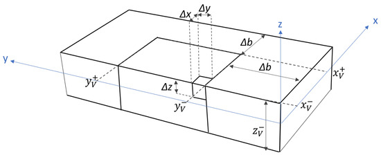
Figure 1.
Schematic representation of the parameters defining the 3D model for the gravity inversion discussed in this paper.
In the next section, criteria to set these parameters will be presented, together with some considerations on the effects of inaccurate choices on the final result.
2. Inversion Parameters Setting
As described in the previous section, when dealing with regional gravity inversion, due to the complexity of the problem, several approximations are required. In the following we analyze all the parameters identified at the end of Section 1, and set them so that the corresponding errors are smaller than the known observation error. For our purpose we will use, as a case study, the inversion of gravity anomalies from a global geopotential model (e.g., the GECO model [14]), synthesized at zero level on an area of 100 km × 100 km, in the Western Mediterranean Sea and centered at and . The target of this example is the crustal structure, i.e., the density distribution from the zero level down to the maximum depth of the Moho (i.e., down to about 22 km ± 2 km accordingly to [15]). We will suppose, in addition, that the observation error has a standard deviation (STD) of 3 mGal with a correlation length of 5 km.
2.1. Model Volume V
Let us start the discussion with the proper setting of the 3D volume V on which the inversion should be performed. We can say that the extreme coordinates in the xy-plane (, and , ) can be easily chosen considering the target of the inversion, while determining the maximum depth is a more difficult task. In this respect, we define two main possibilities.
One possibility could be to set in such a way that the density anomalies below it generate a signal smaller than the observation error (in terms of STD). We will call this depth . In fact, when considering deep density anomalies, density variations became smooth and, due to the large distances from the observation points, they generate an even smoother signal. As a consequence can be chosen as the depth below which the gravitational effect of the density anomalies has a STD smaller than the observation error. These masses can safely be disregarded, since according to Equation (4) the average signal is not fitted in the inversion.
Another possibility could be to consider an a-priori depth (greater than ) and to compute and remove from the observations the gravitational effect of the density anomalies, considered perfectly known, between and .
It can be noted that both approaches require the knowledge of an upper mantle density model: in the former, this model is used just to set and the below density distribution (from to ) is unknown in the inversion, while in the latter, the densities from to are supposed known and their effects are removed from the observations. Since the current knowledge of the mantle density distribution is still uncertain, within this work, we analyzed 11 tomographic models (see Table 1) converted to density models according to different hypothesis for a total of 79 models (see [16] for details).

Table 1.
Mantle models analyzed for the estimate of .
Figure 2 shows the average density and the corresponding STD as functions of depth, computed from the different models in the study region. The two dotted light blue lines represent the mean densities of the upper mantle and of the asthenosphere as provided by the more recent LithoRef18 model [28], here reported only for the sake of comparison.
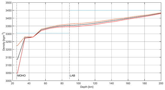
Figure 2.
Average density of the considered models (black solid line) and its 1 accuracy (red solid lines); mean density in the lithospheric upper mantle and in the asthenosphere from the LithoRef18 model [28] (blue dotted line); Moho and lithospheric asthenosphere boundary (LAB) from LithoRef18 (black dashed lines).
To set , one way to proceed is to forward-compute the gravity field of each model, by means of the operator, from a “candidate” , up to a certain maximum depth (e.g., the bottom of the asthenosphere at about 200 km depth). This quantity can be considered to be the error (in mGal) due to the omission, in our model, of the region from to . In Figure 3 the STD of this omission error, for km, is reported in black as a function of different .
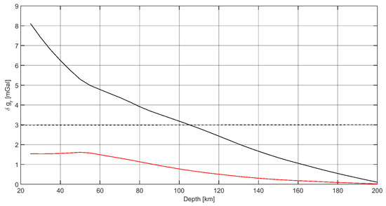
Figure 3.
Omission error STD (black solid line) as a function of the maximum depth of the model and accuracy of the mantle gravitational effect (red solid line) from to a constant as a function of .
It can be noticed that if we suppose an observation error of the order of 3 mGal (dashed line), should be deeper than 110 km. This will guarantee an omission error smaller than the observation error. The red line in Figure 3 represents the propagation (in terms of gravity anomaly) of the uncertainty of global mantle density models from different depths to or, in other terms, the sensitivity of the deep anomaly correction to errors in the lithospheric model. Basically it shows that by computing the effect of different mantle models from a depth of 25 km to a depth of 200 km we have a maximum uncertainty of mGal (which decreases to less than 1 mGal, if we compute it from 100 km to 200 km). Consequently, this means that the gravitational effect of the mantle density distribution from to can be predicted with an accuracy () better than 1.5 mGal (for the current scenario). Since Root et al. [29] showed that in general, available tomographic models are filtered with a 200 km half width Gaussian filter, we evaluate the effect of the presence of high frequencies in the lithosphere by computing the gravitational signal due to random density anomalies with correlation length in the x, y directions of 50 km, an amplitude of 100 kg m and a fixed thickness of 5000 m. It turns out that this perturbation to the initial model produces effects of the order of few tenths of a milligal which are therefore negligible.
With these results in mind, we have two possibilities for our inversion: to extend the maximum depth of the volume V up to 110 km (even if we are interested only in shallower densities), or to remove the effect of the density anomalies taken from one of the above tomographic models up to a certain (thus committing an error of about mGal). Now, since the 1 of the mantle effect (red line in Figure 3) is always smaller than the omission error STD (black line in Figure 3), and taking into consideration also the computational burden required to invert our volume, the latter solution is the preferable one. Please note that of course the above results are strictly dependent on the size of the area of interest (i.e., larger areas will require a deeper volume V), and on the specific region considered (i.e., regions characterized by more rapid density variations inside the mantle will have higher uncertainty and greater STD regarding those shown in Figure 3). From Figure 3 it can also be inferred that in principle, for observations with an accuracy of 1 mGal (typical of airborne gravimetry) the only possibility to keep the model accuracy below the data accuracy, is to extend the inversion volume V up to a depth of 100 km (i.e., up to a depth for which the red line in Figure 3 is below the 1 mGal threshold) and to remove from the observations the effect of remaining part of the upper mantle density anomalies.
We can summarize that in this section we have defined a strategy based on global tomographic mantle models, to set the depth for the inversion model volume V. Moreover, for the current example, aimed to estimate the crustal structure on a region of about 100 km × 100 km from a grid of gravity anomalies at zero level (accuracy of 3 mGal), a maximum depth of 25 km is suitable only if the effect of deeper density anomalies are stripped from the observations.
2.2. Border Size
Once the volume V to be modeled for the inversion is defined, we cannot neglect that important border effects are usually expected. In particular, due to the way in which the volume is modeled we must add, at least in a simplified way, the masses close to the volume boundary up to a certain distance . This is quite obvious if we look at the gravitational effect, shown in Figure 4a, generated by a volume V, with size 100 km in the x and y directions and km, with a constant density of 2670 kg m. It can be clearly seen, from this figure, how the gravitational signal is affected by the lack of masses outside V (the curvature at the extremes is a consequence of this).
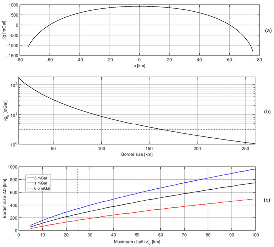
Figure 4.
Gravitational effect generated by a volume V, with size 100 km in the x and y directions and km with a constant density equal to 2670 kg m on a profile in the x direction at the center of V (a); STD of the effect of the borders for the volume V as a function of the border size (b); border size as a function of the maximum depth of V given different observation error STD (c).
Again, the problem of the dimension of the border size () can be solved empirically in a similar way to Section 2.1. Considering a target accuracy given by the observation error, i.e., 3 mGal for our test case, we can start to increase , in such a way that the STD of the gravitational field above V (where we have the gravity observations) is smaller than the target accuracy. In Figure 4b the STD of the effect of the borders (taken here with a constant density of 2670 kg m) for km is represented. It can be seen that for the considered volume depth, a border up to about 165 km is required to guarantee an accuracy of 3 mGal.
Finally, Figure 4c shows the border size as a function of the maximum depth of the volume for three different levels of accuracy, namely mGal, 1 mGal and 3 mGal in blue, black, and red respectively. It can be seen, for instance, that if 1 mGal accuracy is assumed, the border size increases from 165 km to 260 km (it reaches 340 km in case of mGal). Moreover, if the maximum depth for the inversion volume is increased from 25 to 30 km the size of the border increases to 190 km, 300 km and 400 km for the 3 mGal, 1 mGal and mGal accuracy respectively. Please note that is independent from the model resolution , and as well as from the extension of the volume V in the -plane (supposing to have extensions up to a few degrees by a few degrees as stated in the Introduction). With this respect the choice of here presented can be seen as an extension of the work of Szwillus et al. [30] on the importance of far-field effects to the regional/local scale.
Once we have fixed we can investigate the best way to deal with such a border within the data stripping. In doing so, we must consider that usually high-resolution, high-reliability models would probably not be available for that region, due to its dimension and to the fact that it is not the region of interest. So, a possibility could be to use a global crustal model such as CRUST1.0 [31] or LITHO1.0 [32]. However, this solution can be, in terms of computational burden, quite consuming since we must forward-compute the gravity field of a quite large area. Moreover, these global models often do not perfectly join to the more accurate model of the study area, thus introducing unwanted density discontinuities close to the borders of V. A very simple way to proceed consists of extending the a-priori density distribution from the volume V into the border volume by means of a nearest neighbor interpolation. This interpolation has the advantage of giving a density model of the borders which is continuous with that of V and moreover, filling large border areas with constant densities, reduces the computational time required to evaluate its gravitational effect.
To give the reader an example, Figure 5 shows the density model at a depth of 22 km from the CRUST1.0 model (a), and the density model extrapolated by the nearest neighbor algorithm (b). The black rectangles at the center of each map represent the study area. Please note that within this region both the models have the same density.
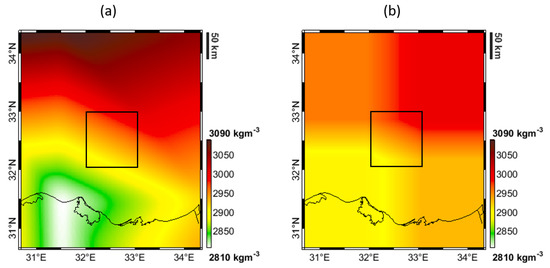
Figure 5.
Density model at a depth of 22 km from the CRUST1.0 model (a), and density model extrapolated by the nearest neighbor algorithm (b). The black rectangles at the center of each map represent the study area.
If we compute the gravitational effect of the CRUST1.0 model and we compare it with the effect of the model from nearest neighbor interpolation we get a STD of the differences of mGal (for a volume V defined as in the previous section). This means that the two models are not significantly different if compared with the observation error of 3 mGal. Of course combined solutions can also be performed: for instance, take the first border of about 10 km from the a-priori model and then extrapolate the rest with the nearest neighbor. For our test case such a mixed solution would reduce the error STD to about mGal.
Concluding this section, we can summarize that from various empirical tests we determine that a border km is required for the inversion of our volume with km. Of all this border the first 10 km can be properly modeled from a prior density model and considered within the inversion, while the remaining part can be fixed and extrapolated with a nearest neighbor algorithm. This procedure will guarantee errors in the inversion due to the border effect smaller than mGal.
2.3. Model Resolution , ,
Once the optimal size of the volume V and of the border have been evaluated, the volume V itself should be discretized, e.g., in a set of rectangular prisms. When dealing with this operation, different factors should be considered:
- the volume of each prism should be small enough to consider constant the mass density within the prism itself;
- , and should be chosen in such a way to have a discretization error smaller than the observation error;
- , and should be chosen in such a way to reduce as much as possible the computational burden;
To evaluate and the easiest way is again by means of an empirical method. We can start by considering an a-priori model with the maximum available resolution (in our example we used as a-priori model the 3D model from [15] with a maximum lateral resolution of 500 m). Then we downsample the model by a factor 2, 3 and 5 obtaining lateral resolutions of 1000 m, 1500 m and 2500 m, respectively. Please note that the number of prisms in the x and y directions decreases from in the initial model to just for the model with resolution 2500 m. In Figure 6 the signal of the a-priori model (a), and its residuals with respect to the signals generated from the different downsampled models (b), (c), and (d) are shown. It can be seen that even considering the 2500 m resolution model (case (d)) the STD of the residuals is of just mGal, which is well below the 3 mGal level. A further downsampling could be possible considering the observation error; however, in this case, we stop the downsampling since the problem has a dimension that can be numerically handled by the inversion SW used.
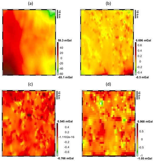
Figure 6.
Signal due to the a-priori model with 500 m resolution (a); its differences with respect to the signal generated from the 1000 m resolution (b), 1500 m resolution (c) and 2500 resolution (d) models.
It must be considered that the sensitivity of the gravitational field in detecting density variations decreases when the distance between the mass source and the observation point increases. As a consequence, when performing the inversion, the densities in the upper part of the model tend to change while the bottom part stays constant [6]. In order to deal with this problem we can set in such a way that each voxel (volume prismatic element) gives the same contribution to the observations. This means choosing such as:
where is the i, j element of the matrix .
Figure 7 shows as a function of depth by imposing that each prism gives the same gravitational effect on the observations of a 100 m thick prism with its top at zero level.
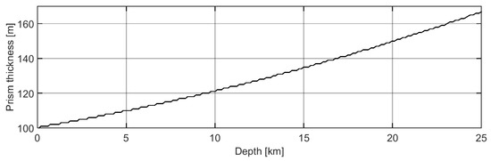
Figure 7.
Prism thickness as a function of depth.
A part regularizing the problem in a way similar to the so-called depth weighting [6,33], the above discretization allows improvement of the computational time, reducing the number of prisms in the z direction, e.g., from 250 to 197 in the current example.
Summarizing, in this section we showed that for the considered scenario, and can be chosen in such a way to reduce the computational burden up to a desired level since they have a minor impact on the accuracy of the model. As for , we have set a rule to increase the prism thickness with depth which regularize the inverse problem and reduce the number of unknowns without affecting the accuracy of the modeling.
The optimal dimensions in which the volume V can be discretized do not greatly affect the solution, in fact even applying different downsampling in the -plane does not significantly change the forward-modeled gravitational signal. As a consequence they can be chosen in such a way to reduce as much as possible the computational burden but always recalling that the volume of each prism should be small enough to consider constant the mass density within the prism itself.
2.4. Data Reduction
The last problem we deal with concerns the data reduction. As recalled in the Introduction, the standard practice is to invert the gravitational field in terms of Bouguer anomalies (), i.e., gravity anomalies () reduced for the effect of the topographic layer ():
The use of is justified because the gravitational effect of the topographic layer is among the largest signals and for sure it is the one at highest frequencies. Moreover, as the geometries of topography and seabed are in general well known from Digital Terrain Models (DTM), their corresponding gravitational effects can be computed in a quite accurate way. However, when selecting the DTM to compute , we must be sure that it is consistent with the observed . In fact gravity anomalies are obtained by means of the application of filters or regularizations to the raw observations and, consequently, they do not contain the full spectrum of the gravitational field. Usually the very-high frequencies are removed. To give an example: let examine a grid of gravity anomalies from a global gravity field model up to degree 2190; it is well known that the maximum spatial resolution achievable is around 10 km half-wavelength [34]. Now, a DTM used to compute the Bouguer anomalies from such a global model should be chosen in such a way that its gravitational effect has a similar spatial resolution. If it is not the case, when applying Equation (6), we will remove the signal frequencies contained in the two terms and , but we will also add the high-frequency content of to (with opposite sign). A possible way to deal with this problem is to compare the stochastic characteristics (e.g., in terms of covariances) of and applying a low-pass filter (e.g., moving average) to the DTM, and therefore smoothing . Figure 8 shows the covariance of (blue line) and of (red line) for the considered example.
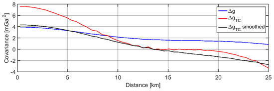
Figure 8.
Covariance of (blue line) of the gravitational effect of the etopo1 model (red line) and of the gravitational effect of the etopo1 model smoothed by means of a moving average with size 5 km (black line).
Here, has been computed from the etopo1 model [35]. It can be seen that has larger amplitudes at the high frequencies. If we apply a moving average with spatial dimension of 5 km, which is quite consistent to the a-priori information of the GECO model, we get a field with similar amplitudes (black line in Figure 8). Please note that here the size of the moving average applied to the DTM is smaller than the global model spatial resolution (i.e., 5 km versus 10 km); however the forward operator, used to compute , acts as a low-pass filter, thus making consistent with . Before concluding this section, we have to observe that in order to deal with the frequency content of the terrain effect, one can think also to compute from a high-resolution DTM and smooth afterwards. This would probably give similar results; however such an approach has the disadvantage that once has been smoothed, we do not know anymore the DTM who is generating it.
In this section, we dealt with the problem of consistency of gravitational signals frequency content that cannot be neglected when performing data reduction. The choice of a DTM with a higher resolution could in fact lead to the introduction, within the observed signal, of unwanted high frequencies. We proposed a method to solve this problem, by the analysis of stochastic characteristics of the signals and the application of a filter to make them consistent.
3. Conclusions
Within this work we have seen that various parameters, namely the size of the volume V to be considered within the inversion (and in particular the maximum depth of V), the size of the borders, the spatial resolution in which V should be discretized and the resolution of a-priori models to be used for the data reduction, should be properly set before dealing with a classical gravity inversion problem. Possible empirical rules to set each of the above-mentioned parameters have been defined. For instance, the classical scenario of retrieving the density distribution within the crust (up to km) on a region of 100 km km, from the inversion of gravity anomalies derived from a high-resolution global model (3 mGal accuracy), requires that:
- we can invert for density anomalies up to a depth of 25 km if we remove from the observations the effect of the density anomalies below 25 km from an a-priori mantle density model (this will entail an error of about mGal);
- we consider borders, in the data reduction, of 165 km around the volume V (this will entail an error of about 3 mGal). The density anomalies in the border can be taken from global models (e.g., CRUST1.0) or even by extrapolating in a constant way the a-priori information available on the density in the volume V;
- V can be discretized on a set of prisms with side 2500 m and a thickness variable between 100 m at the top and 150 m at a depth of 20 km. The discretization in the x and y directions is dictated, in the studied scenario, by the available computational power\time;
- to compute the Bouguer anomaly, we can use the etopo1 model, smoothed with a moving average of size 5 km.
The above findings, outlined for the case study, can be safely applied for inversions with similar characteristics (e.g., area smaller than 100 km × 100 km, depths up to 25 km and observation error of 3 mGal). In other cases the procedure delineated in the paper should be repeated to obtain appropriate values.
Author Contributions
D.S. supervised the study; M.C. and D.S. conceived and performs the study; D.S. and M.C. performs the bibliographic research; M.C. and D.S. wrote the paper.
Funding
This research received no external funding.
Conflicts of Interest
The authors declare no conflict of interest.
References
- Sansò, F.; Capponi, M.; Sampietro, D. Up and Down Through the Gravity Field. In Handbuch der Geodäsie: 6 Bände; Freeden, W., Rummel, R., Eds.; Springer: Berlin/Heidelberg, Germany, 2019; pp. 1–54. [Google Scholar]
- Barzaghi, R.; Sansò, F. Remarks on the inverse gravimetric problem. Boll. Geod. Sci. Aff. 1986, 45, 203–216. [Google Scholar]
- Sampietro, D.; Sansò, F. Uniqueness Theorems for Inverse Gravimetric Problems. In VII Hotine-Marussi Symposium on Mathematical Geodesy; Springer: Berlin, Germany, 2012; pp. 111–115. [Google Scholar]
- Michel, V.; Fokas, A. A unified approach to various techniques for the non-uniqueness of the inverse gravimetric problem and wavelet-based methods. Inverse Probl. 2008, 24, 045019. [Google Scholar] [CrossRef]
- Oldenburg, D.W. The inversion and interpretation of gravity anomalies. Geophysics 1974, 39, 526–536. [Google Scholar] [CrossRef]
- Li, Y.; Oldenburg, D.W. 3-D inversion of gravity data. Geophysics 1998, 63, 109–119. [Google Scholar] [CrossRef]
- Barbosa, V.C.F.; Silva, J.B. Generalized compact gravity inversion. Geophysics 1994, 59, 57–68. [Google Scholar] [CrossRef]
- Reguzzoni, M.; Rossi, L.; Baldoncini, M.; Callegari, I.; Poli, P.; Sampietro, D.; Strati, V.; Mantovani, F.; Andronico, G.; Antonelli, V.; et al. GIGJ: A crustal gravity model of the Guangdong Province for predicting the geoneutrino signal at the JUNO experiment. J. Geophys. Res. Solid Earth 2019, 124, 4231–4249. [Google Scholar] [CrossRef]
- Sampietro, D. GOCE exploitation for Moho modeling and applications. In Proceedings of the 4th International GOCE User Workshop, Munich, Germany, 31 March–1 April 2011; Volume 31. [Google Scholar]
- Nagy, D.; Papp, G.; Benedek, J. The gravitational potential and its derivatives for the prism. J. Geod. 2000, 74, 552–560. [Google Scholar] [CrossRef]
- Moritz, H. The Figure of the Earth: Theoretical Geodesy and the Earth’s Interior; Wichmann: Karlsruhe, Germany, 1990. [Google Scholar]
- Sampietro, D. Geological units and Moho depth determination in the Western Balkans exploiting GOCE data. Geophys. J. Int. 2015, 202, 1054–1063. [Google Scholar] [CrossRef]
- Rossi, L. Bayesian Gravity Inversion by Monte Carlo Methods. Ph.D. Thesis, Politecncico di Milano, Milan, Italy, 2017. [Google Scholar]
- Gilardoni, M.; Reguzzoni, M.; Sampietro, D. GECO: A global gravity model by locally combining GOCE data and EGM2008. Stud. Geophys. Geod. 2016, 60, 228–247. [Google Scholar] [CrossRef]
- Sampietro, D.; Mansi, A.; Capponi, M. Moho depth and crustal architecture beneath the Levant Basin from Global Gravity Field Model. Geosciences 2018, 8, 200. [Google Scholar] [CrossRef]
- Cammarano, F.; Guerri, M. Global thermal models of the lithosphere. Geophys. J. Int. 2017, 210, 56–72. [Google Scholar] [CrossRef]
- Ritsema, J.; Van Heijst, H.J.; Woodhouse, J.H. Global transition zone tomography. J. Geophys. Res. Solid Earth 2004, 109. [Google Scholar] [CrossRef]
- Kustowski, B.; Ekström, G.; Dziewoński, A. Anisotropic shear-wave velocity structure of the Earth’s mantle: A global model. J. Geophys. Res. Solid Earth 2008, 113. [Google Scholar] [CrossRef]
- Boschi, L.; Fry, B.; Ekström, G.; Giardini, D. The European upper mantle as seen by surface waves. Surv. Geophys. 2009, 30, 463–501. [Google Scholar] [CrossRef][Green Version]
- Panning, M.; Lekić, V.; Romanowicz, B. Importance of crustal corrections in the development of a new global model of radial anisotropy. J. Geophys. Res. Solid Earth 2010, 115. [Google Scholar] [CrossRef]
- Grand, S.P. Mantle shear–wave tomography and the fate of subducted slabs. Philos. Trans. R. Soc. Lond. Ser. A Math. Phys. Eng. Sci. 2002, 360, 2475–2491. [Google Scholar] [CrossRef] [PubMed]
- Ritsema, J.; Deuss, A.; Van Heijst, H.; Woodhouse, J. S40RTS: A degree-40 shear-velocity model for the mantle from new Rayleigh wave dispersion, teleseismic traveltime and normal-mode splitting function measurements. Geophys. J. Int. 2011, 184, 1223–1236. [Google Scholar] [CrossRef]
- Lekić, V.; Romanowicz, B. Inferring upper-mantle structure by full waveform tomography with the spectral element method. Geophys. J. Int. 2011, 185, 799–831. [Google Scholar] [CrossRef]
- Debayle, E.; Ricard, Y. A global shear velocity model of the upper mantle from fundamental and higher Rayleigh mode measurements. J. Geophys. Res. Solid Earth 2012, 117. [Google Scholar] [CrossRef]
- French, S.; Lekic, V.; Romanowicz, B. Waveform tomography reveals channeled flow at the base of the oceanic asthenosphere. Science 2013, 342, 227–230. [Google Scholar] [CrossRef]
- Auer, L.; Boschi, L.; Becker, T.; Nissen-Meyer, T.; Giardini, D. Savani: A variable resolution whole-mantle model of anisotropic shear velocity variations based on multiple data sets. J. Geophys. Res. Solid Earth 2014, 119, 3006–3034. [Google Scholar] [CrossRef]
- Ho, T.; Priestley, K.; Debayle, E. A global horizontal shear velocity model of the upper mantle from multimode Love wave measurements. Geophys. J. Int. 2016, 207, 542–561. [Google Scholar] [CrossRef]
- Afonso, J.C.; Salajegheh, F.; Szwillus, W.; Ebbing, J.; Gaina, C. A global reference model of the lithosphere and upper mantle from joint inversion and analysis of multiple data sets. Geophys. J. Int. 2019, 217, 1602–1628. [Google Scholar] [CrossRef]
- Root, B.; Ebbing, J.; van der Wal, W.; England, R.; Vermeersen, L. Comparing gravity-based to seismic-derived lithosphere densities: A case study of the British Isles and surrounding areas. Geophys. J. Int. 2016, 208, 1796–1810. [Google Scholar] [CrossRef]
- Szwillus, W.; Ebbing, J.; Holzrichter, N. Importance of far-field topographic and isostatic corrections for regional density modelling. Geophys. J. Int. 2016, 207, 274–287. [Google Scholar] [CrossRef]
- Laske, G.; Masters, G.; Ma, Z.; Pasyanos, M. Update on CRUST1. 0—A 1-degree global model of Earth’s crust. Geophys. Res. Abstr. 2013, 15, 2658. [Google Scholar]
- Pasyanos, M.E.; Masters, T.G.; Laske, G.; Ma, Z. LITHO1. 0: An updated crust and lithospheric model of the Earth. J. Geophys. Res. Solid Earth 2014, 119, 2153–2173. [Google Scholar] [CrossRef]
- Pilkington, M. 3D magnetic data-space inversion with sparseness constraints. Geophysics 2008, 74, L7–L15. [Google Scholar] [CrossRef]
- Sampietro, D.; Capponi, M.; Mansi, A.; Gatti, A.; Marchetti, P.; Sansò, F. Space-Wise approach for airborne gravity data modelling. J. Geod. 2017, 91, 535–545. [Google Scholar] [CrossRef]
- Amante, C.; Eakins, B.W. ETOPO1 1 aRc-Minute Global Relief Model: Procedures, Data Sources and Analysis; US Department of Commerce, National Oceanic and Atmospheric Administration, National Environmental Satellite, Data, and Information Service, National Geophysical Data Center, Marine Geology and Geophysics Division: Boulder, CO, USA, 2009.


© 2019 by the authors. Licensee MDPI, Basel, Switzerland. This article is an open access article distributed under the terms and conditions of the Creative Commons Attribution (CC BY) license (http://creativecommons.org/licenses/by/4.0/).