Abstract
Water transformation around Antarctica is recognized to significantly impact the climate. It is where the linkage between the upper and lower limbs of the Meridional Overturning Circulation (MOC) takes place by means of dense water formation, which may be affected by rapid climate change. Simulation results from the Community Earth System Model Last Millennium Ensemble (CESM–LME) are used to investigate the Weddell Sea Warm Deep Water (WDW) evolution during the Last Millennium (LM). The WDW is the primary heat source for the Weddell Sea (WS) and accounts for 71% of the Weddell Sea Bottom Water (WSBW), which is the regional variety of the Antarctic Bottom Water (AABW)—one of the densest water masses in the ocean bearing directly on the cold deep limb of the MOC. Earth System Models (ESMs) are known to misrepresent the deep layers of the ocean (below 2000 m), hence we aim at the upper component of the deep meridional overturning cell, i.e., the WDW. Salinity and temperature results from the CESM–LME from a transect crossing the WS are evaluated with the Optimum Multiparameter Analysis (OMP) water masses decomposition scheme. It is shown that, after a long–term cooling over the LM, a warming trend takes place at the surface waters in the WS during the 20th century, which is coherent with a global expression. The subsurface layers and. mainly. the WDW domain are subject to the same long–term cooling trend, which is decelerated after 1850 (instead of becoming warmer like the surface waters), probably due interactions with sea ice–insulated ambient waters. The evolution of this anomalous temperature pattern for the WS is clear throughout the three major LM climatic episodes: the Medieval Climate Anomaly (MCA), Little Ice Age (LIA) and late 20th century warming. Along with the continuous decline of WDW core temperatures, heat content in the water mass also decreases by 18.86%. OMP results indicate shoaling and shrinking of the WDW during the LM, with a ~6% decrease in its cross–sectional area. Although the AABW cannot be directly assessed from CESM–LME results, changes in the WDW structure and WS dynamics have the potential to influence the deep/bottom water formation processes and the global MOC.
1. Introduction
Unique exchange processes and water transformation over the Antarctic continental shelf and shelf slope are contributors in the formation of the Antarctic Bottom Water (AABW), one of the main components of the Meridional Overturning Circulation (MOC) lower limb [1,2,3].
Of all the specific sites around the Antarctic continent, the Weddell Sea (WS) is the primary source of AABW [4,5]—through remote and local water mass interactions influenced by Weddell Gyre (WG) dynamics. More specifically, warm waters being carried eastward by the Antarctic Circumpolar Current (ACC) are captured by the cyclonic WG and transported westward along its southern boundary (Figure 1). This warm water inflow into the WS represents upper and lower varieties of the Circumpolar Deep Water (CDW) which gradually cool and freshen as they entrain the WS ambient waters. By this point they are referred to as the Warm Deep Water (WDW) [6,7,8,9].
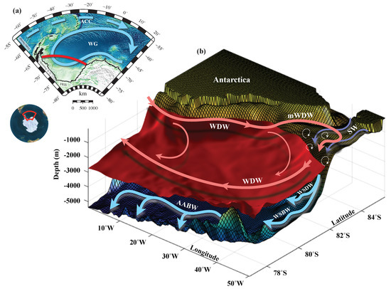
Figure 1.
(a) Atlantic sector of the Southern Ocean topography centered at the Weddell Sea. The full blue arrow represents the Weddell Gyre (WG) circulation and the dashed blue arrow represents the Antarctic Circumpolar Current (ACC) flow. The red line marks the transect assessed with the OMP for WDW investigation throughout the LM, encompassing the inflow and outflow regions of the WG. (b) Perspective of the Weddell Sea multi-layer circulation, depicting the near–shelf break interactions between the WDW (coral arrow) and the super cooled Shelf Waters (SW—purple arrows) to form the WSDW and WSBW, ultimately exported as AABW (light blue arrows).
As WDW interacts with dense shelf waters near the continental WS shelf break, Weddell Sea Bottom Water (WSBW) is formed, the densest AABW regional variety (Figure 1). After further mixing of dense shelf waters with WDW, Weddell Sea Deep Water (WSDW) is produced in a similar manner, the less dense AABW regional variety [10,11].
These deep and bottom waters originated in and exported from the WS represent the major source of the world’s ocean bottom water [7] which eventually spread northward filling all of the abyssal ocean–basins [6,12], underpinning the Southern Ocean (SO) importance in modulating the global MOC [13].
Changes in the SO dynamics and deep water formation that have been reported over the past decades include estimations that the SO has been warming more quickly than the rest of the globe [14,15], reduced salinity/density of sinking waters near Antarctica which are accountable for the formation of AABW [16,17,18,19], as well as freshening of the bottom waters exported from the WS [20].
Although in reality AABW is usually formed when cold dense water spills off the shelf to interact with the WDW and then spreads northwards ventilating the ocean bottom [1,6,7,10], climate–oriented numerical experiments seem unable to fully represent bottom water formation and export in the Southern Ocean [21].
Heuzé et al. [21] investigated the SO bottom water characteristics in CMIP5 models and reported the poor representation of bottom water formation processes in IPCC-class models. Most of these models create deep water by means of open ocean deep convection, a process occurring rarely in reality and highly dependent on polynya events, especially for the inner WS [22,23]. However, coarser-resolution Earth System Models (ESMs) experiments such as CESM–LME are unable to produce open-ocean polynyas in the SO [24,25]. Moreover, ESMs also fail to realistically reproduce the shelf waters in the SO in part due to the lack of ice shelf parameterizations, which has been achieved in high resolution experiments with thermodynamically active ice shelves [26,27]. Finally, due to its large heat capacity and weak thermal connection to the surface, the deep ocean typically requires millennia of spin-up integration of an ESM with constant atmospheric composition to reach an approximately steady state [28,29,30].
Within this scenario, the participation of the WDW plays a central role. It is estimated that 71% of the WSBW is composed of WDW compared with only 29% of dense shelf waters (SW) [31]. Variations in the WDW and its dynamics can give us insights into the SO contribution to the deep overturning circulation and the meridional transport of heat and properties which impact the climate system as a whole. Therefore, a more reliable approach to assess the potential impacts of climate variability upon the bottom water formation in the SO from global numerical experiments is to examine the upper component of the deep meridional overturning cell, i.e., the WDW [32].
Variations in WDW properties might be imparted mainly by variations in the CDW inflow at the boundary of the WG, which in turn are promoted by changes in atmospheric forcing conditions, more specifically the Southern Annular Mode (SAM; [32]). The SAM is the most important atmospheric mode of climate variability in the Southern Ocean [33,34]. It modulates the path of the westerly winds and changes in mixed layer depths [35], and seems to be correlated with the WSBW variability [36]. Since the WDW is one of the source components of bottom water, the variations of the two water masses are possibly related through the formation process [32].
Mixing processes between recirculated waters and WS cooler waters can also contribute to WDW variability and change [32,37]. Both these studies use a set of observational data measurements collected in the WS on the Greenwich Meridian (GM). Furthermore, Fahrbach et al. [32] demonstrate that asymmetric wind forcing at the northern and southern limbs of the WG result in variable inflow/outflow at the open boundaries of the gyre. In order to compensate for these variations, WG internal processes act to redistribute the heat and salt anomalies therein, resulting in long-term trends in temperature and salinity in the whole water column of the gyre [32].
The Last Millennium (LM) represents an interesting framework for assessing the relevance of modern climate changes [38,39,40,41]. Among all past time-scales, the LM comprises a shorter time interval closest to the recent past.
Principal boundary conditions on the climate (e.g., Earth orbital geometry and global ice mass) have not changed appreciably since the LM. Thereby, in the absence of any human influence, the natural climate variability that might be expected over the present century is likely to be represented by the observed variations in climate over this time frame [39]. The LM gives us therefore the opportunity to understand the underlying background record of forcing and climate system response, regardless of how anthropogenic effects develop in modern climate variations [41].
Two prominent climatic events resulting from natural variability punctuate the LM: the Medieval Climate Anomaly (MCA), from 950 to 1250, and the Little Ice Age (LIA), from 1400 to 1700 [42]. These correspond to relative warm and cold hemispheric conditions, respectively, which were distinct with regard to estimated external radiative forcing of the climate [43]. Despite existing MCA and LIA heterogeneity through time and space, reconstructions show generally warm and cold conditions, respectively, encompassing these periods [44], while individual proxy series and hemispheric/global composites ensure a robust view of global–scale changes [39].
Here we explore the WDW evolution throughout the LM using the simulation results from the Community Earth System Model Last Millennium Ensemble (CESM-LME) experiment [45]. We refer to the LM as the entire 850–2006 period, encompassing both the 850–1850 pre-industrial and the 1850–2006 post-industrial eras.
This work is organized as follows. Section 2 provides a brief description of the model data used and methods. Section 3 presents the model simulation results. Section 4 summarizes and discusses the results while Section 5 presents a brief conclusion. Finally, a list of major acronyms is also included at the end of Section 5.
2. Data and Methods
The CESM-LME experiment includes a set of simulations forced with reconstructions for the transient evolution of solar intensity, volcanic emissions, greenhouse gases, aerosols, land use conditions, and orbital parameters, both together and individually, for the period of 850–2006. It uses a two–degree nominal resolution in the atmosphere and land components and one–degree nominal resolution in the ocean and sea ice components. The CESM 1.1 version used in this experiment is fully documented in [46]. Details on the ocean model, which has 60 vertical levels, are described in [47]. The model is first spun up for a year 1850 control simulation of 650 years and then a year 850 control simulation is branched from there and run for more 1356 years. All CESM–LME simulations were started from year 850 of the 850 control simulation (detailed in Figure 1 from Otto-Bliesner et al. [45]). Output from the ensemble members are available through the Earth System Grid (http://www.earthsystemgrid.org) as single variable time series. This study examines the ensemble–mean of 13 members with the full–set of external forcings.
The forcings are applied identically across ensemble members. The only difference among these experiments is the application of a random round-off difference in the air temperature field that initializes each experiment, which will eventually result to an ensemble spread. The spread of trends across the ensemble indicates how much internal variability causes individual ensemble members to deviate from the forced trend. The calculation of the ensemble mean therefore averages out natural climate variability and thus represents the forced climate response. For more details, the reader is referred to the overview paper of the Last Millennium Ensemble Project [45].
The CESM–LME has been recently used in a wide range of studies of climate variability and change (e.g., [48,49,50,51] and many more that are listed in the CESM-LME publications page [52]), which have extensively tested the model results against other ESMs of the CMIP5, for example [53], and have also shown that the full-forcing realizations reproduce major modes of observed internal climate variability [54,55,56,57]. In fact, the CESM model scores among the best models in representing major modes of climate variability [58]. These set of studies have proven the CESM-LME usefulness in detecting different climate change signals across the globe.
Potential temperature () outputs from the CESM–LME simulation are firstly used to assess the water column structure along a transect across the WS (Figure 1). Temperature anomalies are computed for the late 20th century (1970–2000, as in [59]) and for the contrasting periods of the MCA (950–1250) and LIA (1400–1700), following the definitions of Mann et al. [42] in terms of distinct three–century–long periods. The MCA and LIA spatial patterns are not sensitive to precise time intervals used to define them, according to these authors.
To investigate the spatial–temporal variation of the WDW, the Optimum Multiparameter Analysis (OMP) water mass decomposition scheme is used to determine the WDW contribution (%) along the WS transect (Figure 1), comprising the inflow and outflow regions of the WG. The ocean heat content (OHC) is computed within the WDW transect area, i.e., where the WDW contributions are above 50%. The WDW variability is assessed by means of time series of the water mass core potential temperature (), here defined as the median of the 30% warmest grid points of the WS transect (i.e., above the 70th percentile of ). Additionally, time series of the barotropic streamfunction (BSF) at the southern boundary of the WG (coinciding with the inflow of the WDW) and the WS sea ice extent anomalies are analyzed.
Optimum Multiparameter Analysis—OMP
The OMP analysis was introduced by [60] as an alternative option to expand the classic triangle mixing from T/S diagrams. The method is based on a linear mixing model, where every property of one water mass is subjected to the same mixing processes and present the same turbulent mixing coefficients, yielding relative fractions of a mixture (or contribution in % to the total mixture) of distinct water masses through the linear system of equations. It uses conservative and non–conservative sea water parameters to solve a linear system of mixing equations (e.g., Equation (1), [61,62,63]).
The OMP estimates the contribution of seawater properties that represent a water mass in its source region (Source Water Types – SWT) in a water sample that represents an original water mass, with no mixing. Every water sample is represented by a linear combination of SWTs, with well known properties. OMP does not actually solve the linear system (1). Instead, it tries to estimate the best collection of contributions (x) from all SWTs, by minimizing the residuals (R) subjected to certain conditions: the sum of every SWTs contribution must be 100% (mass conservation) and there can not be negative contributions, since the smallest contribution must be zero [63].
The equations allow an objective evaluation of the solution quality. The system can be weighted to adjust the representativeness of each parameter, so the mass conservation residuals objectively indicate the quality of the solution [31,63,64]. Low residuals suggest that the samples are well represented by the SWT collection [65,66].
Following Kerr et al. [4], –S diagrams are evaluated to extract SWTs for the Antarctic Surface Water (AASW), WDW and AABW.AASW was used to separate the warm and salty WDW from the cold and lighter surface water, whereas AABW isolates the slightly colder deep layers. Amongst several variables, CESM–LME provides potential temperature and salinity outputs from the oceanic component which, together with the potential vorticity (PV) computed by OMP, permits the separation of three water masses using the OMP linear equation system. Following Kerr et al. [31], and S are given the same weight (here W = 10) whilst PV is given a much smaller significance (W = 1 × 10), since it is used to close the linear equation system. We adopt a Monte Carlo approach to produce random perturbations on the SWTs and the upper limit in residuals (5%) of mass conservation is used to remove regions poorly represented [65,66].
3. Results
As a first approach to assess the water column structure of the WS throughout the LME simulation, we examine the potential temperature anomaly along the WS transect during the MCA (950–1250) and the LIA (1400–1700), as well as the late 20th century (1970–2000) with regards to the pre-industrial LM base period (850–1850).
Figure 2 presents the potential temperature anomaly along the WS transect for the MCA (Figure 2a), LIA (Figure 2b) and late 20th century (Figure 2c). During the MCA, the entire water column is warmer than the base period, with more intense anomalies located above the 2000 m depth (≈+0.07 C). During the LIA, the opposite anomaly distribution is observed, where the water column is almost entirely colder than in the pre–industrial LM, especially above 2000 m (≈−0.05 C), except for the bottom layers which still show positive temperature anomalies. Finally, the late 20th century displays a very interesting spatial pattern. While the surface layers are subject to quite intense warm anomalies (≈+0.15 C), the subsurface down to 2000 m, precisely within the WDW domain, displays an explicit cold anomaly just as intense in magnitude (≈−0.15 C).
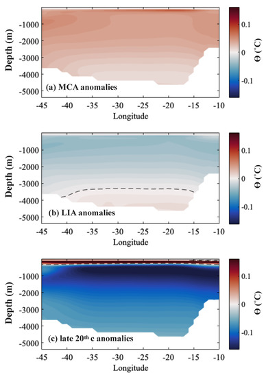
Figure 2.
Potential temperature anomalies along the WS transect (C) with respect to the pre–industrial Last Millennium (LM) base period (850–1850): (a) Medieval Climate Anomaly (MCA), between 950–1250; (b) Little Ice Age (LIA), between 1400–1699 and (c) late 20th century (Present), between 1970–1999 (in line with [59]). Warm/cold colors represent positive/negative anomalies. Black dashed lines represent the zero contour of anomalies.
To investigate the multilayer distinct behavior of potential temperature along the WS transect, we compute the vertically integrated temperature anomalies at the surface (5–200 m) and subsurface layers (300–700 m), both zonally averaged within the WS transect. Figure 3a,b present surface/subsurface potential temperature anomalies (detrended and normalized by the standard deviation) from 1050 to 2006. Similarly, Figure 3c displays the sea ice extent anomalies computed for the WS (50–90 S & 60 W–20 E) for the same LM period. Following [59], the time series start in year 1050, considering that the CESM–LME is still drifting during the first 200 years of the LME simulation.
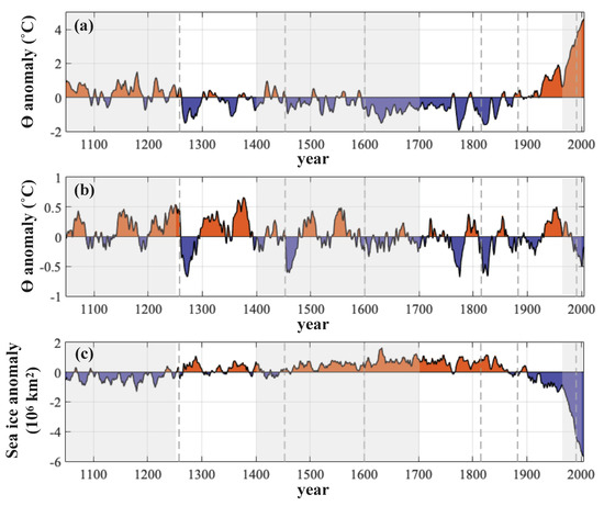
Figure 3.
Time series of zonally averaged potential temperature anomalies along the WS transect and sea ice extent anomalies with respect to the full LME simulation period. (a) Vertically integrated surface layers (5–200 m). In the same fashion, (b) refers to integrated subsurface layers (300–700 m). (c) Horizontally averaged sea ice extent within the WS (50–90 S & 60 W–20 E). Anomalies are detrended and normalized by the standard deviation. Light gray shaded areas refer to the MCA, LIA and late 20th century, as in Figure 2. Dashed gray lines mark major volcanic eruptions: Samalas, 1258; Kuwae, 1453; Huaynaputina, 1600; Tambora, 1815; Krakatoa, 1883; Pinatubo, 1991.
Both surface and subsurface time series (Figure 3a,b) suggest an overall cooling trend throughout the LME simulation, which is consistent with global temperature trends computed for the LM by previous studies [44,67,68,69] and the CESM-LME full and individual forcings Diagnostics Package [70]. The MCA warm signature is also evident in both layers, denoted by the positive anomalies in Figure 3a,b and the negative sea ice extent anomalies (Figure 3c). The LIA relative cooling is somewhat observed in the surface and in the sea ice positive anomalies, but with no clear signal in the subsurface. By entering the post–industrial period and mainly the 20th century, the surface potential temperatures undergo an abrupt increase (Figure 3a), which is mirrored by an intense decline in sea ice extent (Figure 3c).
During the the late 20th century, the surface is subject to intense warming, which actually builds up from the early century. This is consistent with the CESM–LME diagnostics [70] and pinpoints the impact of greenhouse gases (GHG) forcing, which not only hampers the overall cooling by the end of the LM (both globally and regionally), but actually provokes an opposing trend during the entire 20th century.
Although this intense 20th century warming trend is not clearly observed within the subsurface layers, it is interesting to notice that the cooling response to large eruptions seem to play a role in the subsurface temperature variability within the WS. Most of the major volcanic events (pinpointed by gray dashes lines) are followed by a postevent cooling (Figure 3), which is consistent with Landrum et al. [57], who reported global and hemispheric cooling responses of the CCSM4 (single–run experiment) to large eruptions of the LM. The immediate impacts of explosive volcanism on global surface climate has been well documented and intensively investigated (e.g., Robock [71] and references therein). Large volcanic eruptions are known to produce maximum surface cooling in the polar regions due to the positive feedback of sea ice [71]. Surface temperatures seem to respond directly to the postevent sea ice extent increase, whilst the subsurface temperature anomalies exhibit the global expression also imprinted in the ACC. The mild response at the surface for the later part of the 20th century is masked by the GHG-related intense warming.
Bearing in mind the origins of the WDW, which derives from the CDW captured from the ACC [6,8,72], these signals are likely to be imported from lower latitudes and carried into the WS deep layers by the WG circulation. Subsurface potential temperature anomalies computed for the ACC and for the southern limb of the WG along the Greenwich Meridian (Figure S1a,b), consistent with [32,37], suggest that ACC temperatures follow the global cooling trend during the LM (≈0.2 C) as well as the 20th century warming trend. The southern limb of the WG at the GM, on the other side, displays the same pattern observed in the subsurface of the WS transect (Figure 3b), where the GHG forcing impacts are imprinted as a decelerated cooling trend, instead of the warming trend observed in the ACC, probably resulting from the interactions with sea ice-insulated ambient waters.
To further assess whether the WDW spatial distribution is affected during the LME simulation period, the OMP water masses decomposition scheme is applied to potential temperature and salinity results from the WS transect. Several time slices of the LM are analyzed. To each time period assessed, –S diagrams are used to extract the Source Water Types that represent each water mass, i.e., AASW, WDW and AABW (Table 1).

Table 1.
Ensemble mean Sea Water Types extracted from –S diagrams for AASW, WDW and AABW used in OMP analysis for specific time slices/ranges of the CESM-LME experiment simulation period.
Figure 4 displays the OMP results for the most contrasting time slices assessed, the initial and final phases of the LME simulation, i.e., years 1050 and 2000. Consistent with Wainer and Gent [59], we disregard the first 200 years of the LME simulation to perform the OMP and WDW core analysis, since the CESM–LME is still drifting, hence year 1050 representing the initial phase of the LM.
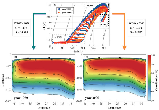
Figure 4.
(a) –S diagram for the initial/final phases of the LME simulation, i.e., year 1050 (blue markers) and year 2000 (red markers). The left/right text boxes show the Source Water Types applied to OMP, provided in detail in Table 1. (b) Warm Deep Water percentage contribution above 50% (colors and solid lines) along the Weddell Sea transect from the OMP decomposition scheme: (b) represents year 1050 and (c) represents year 2000. Throughout the simulation period, the WDW transect area shrinks by 6.3% followed by a OHC decrease of 18.86%.
Consistent with the potential temperature anomalies presented in Figure 2, the –S diagram in Figure 4 for the initial/final phases of the LME simulation (blue/red markers) suggests that the WDW became colder and slightly saltier during the LM. The side text boxes show the SWTs derived from the –S diagram and used to run the OMP analysis for these two time-slices. The lower panels present the WDW percentage contribution above 50% (colors and solid lines) along the WS resulting from the OMP decomposition scheme: (b) for the year of 1050 and (c) for the year of 2000.
First thing to be noticed is that during the LM, the WDW cross-section area shrinks about 6.3% between the years 1050 and 2000. The OHC computed within the WDW cross-section area decreases about 18.86% between 1050 and 2000. Finally, the WDW shrinking trend is accompanied by the shoaling of the water mass, whose core (computed within the contribution >90% area) becomes ≈120 m shallower by the end of the LME simulation period.
Onto the investigation of the WDW variability, Figure 5 displays a set of time series focusing on the WDW core potential temperature and the barotropic streamfunction (BSF) variation during the LME simulation. Figure 5a displays the temporal variation of the zonally averaged temperature profile at the WS transect. The most prominent feature is the temperature decrease of ≈0.2 C during the LM at 500 m, which is more precisely the WDW core depth according to the OMP analysis (Figure 4). No clear variation is observed at the surface.
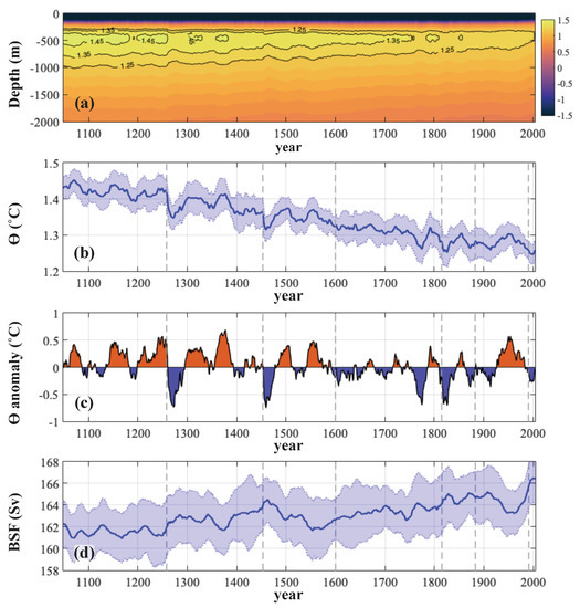
Figure 5.
(a) Temporal variation throughout the simulation period (1050–2006) of the zonally averaged potential temperature of the WS transect between the surface and 2000 m, encompassing the WDW domain. The isotherms of 1.25 C, 1.35 C and 1.45 C are marked by solid black lines to highlight the changes in the WDW core temperature. (b) Variation of the WDW core potential temperature defined as the 30% warmest grid points in the WS transect (>70th percentile of ). The solid blue line and the light blue shaded area represent the ensemble mean and the 13–member spread, respectively. (c) WDW core potential temperature detrended anomalies throughout the simulation period. (d) Variation of the barotropic streamfunction (Sv) of the southern limb of the WG. The solid blue line and the light blue shaded area represent the ensemble mean and the 13-member spread, respectively. Dashed gray lines mark major volcanic eruptions: Samalas, 1258; Kuwae, 1453; Huaynaputina, 1600; Tambora, 1815; Krakatoa, 1883; Pinatubo, 1991.
Figure 5b,c display the time series of the potential temperature and its anomaly, respectively (with respect to the pre-industrial LME simulation period) for the WDW core computed as the 30% warmest grid points in the WS transect (>70th percentile of ). Once again, the long–term cooling trend over most of the LM is consistent with a global expression, which is part of a multimillennial trend that extends far back the beginning of the Common Era (CE) [44,69,73,74,75,76,77]. The cooling trend is steepest for the 1000–1800 CE interval [69] and it has been attributed to solar, orbital and volcanic natural external forcings [44,67,68,69] (also demonstrated by the CESM–LME full and individual forcings Diagnostics Package [70]), with a significant contribution from internal, unforced climate variability [78,79]. Nevertheless, during the 20th century the cooling trend is decelerated possibly as a buffered fingerprint of the GHG–related global warming trend pinpointed by the CESM-LME Diagnostics Package [70]).
Figure 5d displays the time series for the barotropic stream function (BSF) for the southern boundary of the WG, coinciding with the inflow of the WDW. Although two somewhat prominent regime shifts occur after 1450 and ≈1850, the BSF displays an overall positive trend, suggesting the intensification of the WG throughout the LM.
4. Discussion
The Warm Deep Water is investigated throughout the Last Millennium from the simulation results of the 13-member ensemble CESM-LME experiment with respect to a transect crossing the Weddell Sea (Figure 1). The most evident feature shown is a long–term cooling along the WS transect during the LM, which is consistent with a global cooling trend indicated by the CESM-LME full and individual forcings Diagnostics Package [70], as well as with a multimillennial global expression extending far back the beginning of the Common Era (CE) [44,69,73,74,75,76,77]. The enhanced cooling during the LM has been attributed to solar, orbital and volcanic natural external forcings [44,67,68,69], with a significant contribution from internal, unforced climate variability [78,79].
Signatures of the warm-MCA and the cold-LIA are observed along the WS transect (Figure 2), consistent with previous numerical [57] and proxy-based investigations of the LM period [42,43,75,80,81,82,83], even though the later being reliable only for the Northern Hemisphere. The late 20th century, however, displays a vertically divergent pattern. Whilst the surface is subject to an intense warming (which actually builds up from the early century due to GHG forcing), the deeper layers preserve the cooling trend, although decelerated during the 20th century (Figure 5b), almost to the very end of the LME simulation, this cooling being more intense within the WDW domain, i.e., between 300 m and 2000 m (Figure 2).
The intense warming observed at the WS surface layers after ≈1850 (Figure 3a) is associated with negative sea ice extent anomalies in the WS (Figure 3c), both time series clearly reflecting the strengthened GHG forcing in the 20th century, which also displays a global signature [70]. Even though GHG forcing seems unable to provoke the same temperature opposing trend at the WS subsurface layers (Figure 3b), it is strong enough to weaken the steep cooling trend observed until the early 20th century (Figure 5b). Despite the apparent sea ice insulation, negative temperature anomalies for both surface and subsurface reveal local and global effects of large volcanic eruptions: while surface postevent cooling reflects the positive sea ice feedback [71], subsurface temperature anomalies echo the global cooling signal [57,70] originated in lower latitude waters from ACC.
The OMP analysis results indicate the WDW to become shallower and thinner by the end of the LM (Figure 4). During the LM, the WDW cross-section area shrinks about 6.3% between the years 1050 and 2000 and the OHC computed within the WDW cross-section area decreases about 18.86%. The WDW shrinking trend is accompanied by the shoaling of ≈120 m of the water mass core depth.
From the time series presented in Figure 5a–c, it is clear that the WDW core undergoes a long-term cooling throughout the LM until ≈1850, when this cooling trend slows down due to the enhanced GHG forcing, which is highlighted by the positive surface temperature anomalies, as well as the negative sea ice extent anomalies, in Figure 3. Although the GHG signature can also be observed in the ACC subsurface waters (Figure S1a), from which the WDW originates, the local dynamics seem to temper the intense warming yielding the decelerated cooling trend. As described by Robertson et al. [9], the WDW cools down as it transits the WG, primarily through mixing with cooler ambient waters. These interactions, together with sea ice insulation, seem to buffer the intense post-industrial warming observed at the WS surface waters (Figure 3), as well as in ACC subsurface waters (Figure S1a), which have also been reported by observation–based studies [9,14,15].
The potential impacts of such variability of the WDW on the AABW formation are somewhat puzzling. Although the AABW cannot be directly assessed from CESM-LME results, for instance, for being way too warm when compared to observations from Robertson et al. [9] and Gouretski and Koltermann [84], the contribution of the WDW in this scenario is unequivocal [2,4,5,31]. Kerr et al. [31] reported the WSBW—the densest AABW regional variety—to be composed by 71% of WDW and 29% of dense shelf waters (SW). Ergo, changes in these WSBW precursors would ultimately be modulating the AABW variability [32], either by means of a reduction/expansion in the formation rate or by shifting to the production of a less/more dense variety of bottom water, or even by a combination of both mechanisms [85].
The shrinking of WDW could indicate a smaller volume of WDW to be entering the WS, hence decelerating the formation of the AABW. However, BSF time series (Figure 5) suggests that the WG intensifies over the entire LME simulation, thus transporting more WDW into the WS. Moreover, WDW becomes colder and slightly saltier (i.e., denser), which leads to increased potential instability, favouring deep convection. Therefore, due to OMP mass conservation restrain (i.e., the sum of every SWT contribution must be 100%), the observed shoaling and thinning of WDW during the LME simulation seems to be associated with an enhanced bottom water production.
The CESM-LME experiment provides a good understanding of the Southern Ocean behavior under the pre-industrial natural forced scenario of the LM, especially with respect to the mid-to-deep layers circulation. Similar experiments spanning the 21st century, such as the CESM Large Ensemble Project (LENS) and the CMIP6-ScenarioMIP projections, shall provide deeper insights on the climate change impacts on the SO dynamics, especially in terms of anthropogenic forcing.
5. Conclusions
We have investigated the spatial–temporal variation of the Warm Deep Water during the Last Millennium. The WDW accounts for 71% of the Antarctic Bottom Water formation within the Weddell Sea [31], bearing directly with the global Meridional Overturning Circulation. Outputs from the CESM-LME referring to a transect across the Weddell Sea were assessed with the OMP analysis along with potential temperature time series to determine the WDW behavior throughout the LM.
The evolution pattern of potential temperature along the WS transect is clear throughout the three major LM climatic episodes, i.e., MCA, LIA and the 20th century warming. Both surface and subsurface capture the postevent cooling signature after major volcanic eruptions during the LM.
After a long–term cooling over the LM, a warming trend takes place at the surface waters in the 20th century parallel to the sea ice extent decline in the WS, both associated with anthropogenic GHG forcing, coherent with a global expression. The subsurface layers and mainly the WDW domain do not show the opposing trend observed at the surface in the 20th century. Rather, the WDW long-term cooling trend is only softened after 1850, probably due to interactions with cooler sea ice-insulated ambient waters, that seemingly buffer the strong warming signal.
OMP results suggest the shoaling of the WDW throughout the LM associated with mild shrinking of the water mass (about 6% of its cross-sectional area). Besides the shrinking trend, the WDW ocean heat content decreases by 18.86% during the LME simulation period, which is associated with the WDW core cooling and shallowing.
The strengthening of Weddell Gyre barotropic streamfunction indicates the sustained input of WDW over the LM. Therefore, although the AABW cannot be directly assessed from CESM-LME results (as in most ESMs), the WDW shrinking might be associated with enhanced bottom water production favoured by potential instability due to the input of a cooler (and denser) WDW. Hence, given the unequivocal relevance of the WDW to the AABW formation and ultimately the global MOC, this study provides the basis for further investigations related to the WDW and the future of global climate.
Supplementary Materials
The following are available online at https://www.mdpi.com/2076-3263/9/8/346/s1. Figure S1: Meridionally averaged potential temperature anomalies time series along the Greenwich Meridian: (a) the ACC (47–52S); (b) the southern limb of the WG (62–67S). Anomalies are detrended and normalized by the standard deviation. Light gray shaded areas refer to the MCA, LIA and late 20th century, as in Figure 2 in the manuscript. Dashed gray lines mark major volcanic eruptions: Samalas, 1258; Kuwae, 1453; Huaynaputina, 1600; Tambora, 1815; Krakatoa, 1883; Pinatubo, 1991.
Author Contributions
Conceptualization, M.T. and I.W.; Methodology, M.T. and B.F.; Software, M.T. and B.F.; Validation, M.T., F.M., B.F. and I.W.; Formal Analysis, M.T. and B.F.; Writing—Original Draft Preparation, M.T. and F.M.; Writing—Review & Editing, M.T., F.M., B.F. and I.W.; Visualization, M.T. and B.F.; Supervision, I.W.; Project Administration, M.T. and I.W.; Funding Acquisition, M.T. and I.W.
Funding
This study was financed in part by the grants FAPESP: #2015/17659–0, #2017/16511–5; CNPq: #301726/2013–2, #405869/2013–4; CNPq–MCT–INCT–594 CRIOSFERA 573720/2008–8 and Coordenação de Aperfeiçoamento de Pessoal de Nível Superior–Brasil (CAPES)–Finance Code 001; CAPES 88887.318265/2019-00.
Acknowledgments
The CESM project is supported primarily by the National Science Foundation (NSF). This material is based upon work supported by the National Center for Atmospheric Research (NCAR), which is a major facility sponsored by the NSF under Cooperative Agreement No. 1852977. Computing and data storage resources, including the Cheyenne supercomputer (doi:10.5065/D6RX99HX), were provided by the Computational and Information Systems Laboratory (CISL) at NCAR.
Conflicts of Interest
The authors declare no conflict of interest. The funders had no role in the design of the study; in the collection, analyses, or interpretation of data; in the writing of the manuscript, or in the decision to publish the results.
Abbreviations
The following abbreviations are used in this manuscript:
| AABW | Antarctic Bottom Water |
| ACC | Antarctic Circumpolar Current |
| AMOC | Atlantic Meridional Overturning Circulation |
| CDW | Circumpolar Deep Water |
| CESM–LME | Community Earth System Model Last Millennium Ensemble (experiment) |
| FRIS | Filchner–Ronne Ice Shelf |
| LIA | Little Ice Age |
| LM | Last Millennium |
| MCA | Medieval Climate Anomaly |
| MOC | Meridional Overturning Circulation |
| OMP | Optimum Multiparameter Analysis |
| PV | Potential Vorticity |
| SO | Southern Ocean |
| SWT | Source Water Types |
| WDW | Warm Deep Water |
| WG | Weddell Gyre |
| WS | Weddell Sea |
| WSBW | Weddell Sea Bottom Water |
| WSDW | Weddell Sea Deep Water |
References
- Orsi, A.H.; Jacobs, S.S.; Gordon, A.L.; Visbeck, M. Cooling and ventilating the abyssal ocean. Geophys. Res. Lett. 2001, 28, 2923–2926. [Google Scholar] [CrossRef]
- Orsi, A.H.; Smethie, W.M., Jr.; Bullister, J.L. On the total input of Antarctic waters to the deep ocean: A preliminary estimate from chlorofluorocarbon measurements. J. Geophys. Res. Ocean. 2002, 107, 31-1–31-14. [Google Scholar] [CrossRef]
- Talley, L.D. Closure of the global overturning circulation through the Indian, Pacific, and Southern Oceans: Schematics and transports. Oceanography 2013, 26, 80–97. [Google Scholar] [CrossRef]
- Kerr, R.; Heywood, K.; Mata, M.; Garcia, C. On the outflow of dense water from the Weddell and Ross Seas in OCCAM model. Ocean Sci. 2012, 8, 369–388. [Google Scholar] [CrossRef]
- Van Sebille, E.; Spence, P.; Mazloff, M.R.; England, M.H.; Rintoul, S.R.; Saenko, O.A. Abyssal connections of Antarctic Bottom Water in a Southern Ocean state estimate. Geophys. Res. Lett. 2013, 40, 2177–2182. [Google Scholar] [CrossRef]
- Orsi, A.H.; Nowlin, W.D., Jr.; Whitworth, T., III. On the circulation and stratification of the Weddell Gyre. Deep Sea Res. Part I Oceanogr. Res. Pap. 1993, 40, 169–203. [Google Scholar] [CrossRef]
- Fahrbach, E.; Rohardt, G.; Scheele, N.; Schröder, M.; Strass, V.; Wisotzki, A. Formation and discharge of deep and bottom water in the northwestern Weddell Sea. J. Mar. Res. 1995, 53, 515–538. [Google Scholar] [CrossRef]
- Naveira Garabato, A.C.; McDonagh, E.L.; Stevens, D.P.; Heywood, K.J.; Sanders, R.J. On the export of Antarctic bottom water from the Weddell Sea. Deep Sea Res. Part II Top. Stud. Oceanogr. 2002, 49, 4715–4742. [Google Scholar] [CrossRef]
- Robertson, R.; Visbeck, M.; Gordon, A.; Fahrbach, E. Long-term temperature trends in the deep waters of the Weddell Sea. Deep Sea Res. Part II Top. Stud. Oceanogr. 2002, 49, 4791–4806. [Google Scholar] [CrossRef]
- Jullion, L.; Garabato, A.C.N.; Bacon, S.; Meredith, M.P.; Brown, P.J.; Torres-Valdés, S.; Speer, K.G.; Holland, P.R.; Dong, J.; Bakker, D.; et al. The contribution of the Weddell Gyre to the lower limb of the Global Overturning Circulation. J. Geophys. Res. Ocean. 2014, 119, 3357–3377. [Google Scholar] [CrossRef]
- Nicholls, K.; Østerhus, S.; Makinson, K.; Gammelsrød, T.; Fahrbach, E. Ice-ocean processes over the continental shelf of the southern Weddell Sea, Antarctica: A review. Rev. Geophys. 2009, 47, RG3003. [Google Scholar] [CrossRef]
- Mantyla, A.W.; Reid, J.L. On the origins of deep and bottom waters of the Indian Ocean. J. Geophys. Res. Ocean. 1995, 100, 2417–2439. [Google Scholar] [CrossRef]
- Sloyan, B.M.; Rintoul, S.R. The Southern Ocean limb of the global deep overturning circulation. J. Phys. Oceanogr. 2001, 31, 143–173. [Google Scholar] [CrossRef]
- Gille, S.T. Warming of the Southern Ocean since the 1950s. Science 2002, 295, 1275–1277. [Google Scholar] [CrossRef] [PubMed]
- Gille, S.T. Decadal-scale temperature trends in the Southern Hemisphere ocean. J. Clim. 2008, 21, 4749–4765. [Google Scholar] [CrossRef]
- Jacobs, S.S. Bottom water production and its links with the thermohaline circulation. Antarct. Sci. 2004, 16, 427–437. [Google Scholar] [CrossRef]
- Jacobs, S. Observations of change in the Southern Ocean. Philos. Trans. R. Soc. A Math. Phys. Eng. Sci. 2006, 364, 1657–1681. [Google Scholar] [CrossRef]
- Aoki, S.; Bindoff, N.L.; Church, J.A. Interdecadal water mass changes in the Southern Ocean between 30∘ E and 160∘ E. Geophys. Res. Lett. 2005, 32. [Google Scholar] [CrossRef]
- Rintoul, S.R. Rapid freshening of Antarctic Bottom Water formed in the Indian and Pacific oceans. Geophys. Res. Lett. 2007, 34. [Google Scholar] [CrossRef]
- Jullion, L.; Naveira Garabato, A.C.; Meredith, M.P.; Holland, P.R.; Courtois, P.; King, B.A. Decadal freshening of the Antarctic Bottom Water exported from the Weddell Sea. J. Clim. 2013, 26, 8111–8125. [Google Scholar] [CrossRef]
- Heuzé, C.; Heywood, K.J.; Stevens, D.P.; Ridley, J.K. Southern Ocean bottom water characteristics in CMIP5 models. Geophys. Res. Lett. 2013, 40, 1409–1414. [Google Scholar] [CrossRef]
- Carsey, F.D. Microwave Observation of the Weddell Polynya. Mon. Weather Rev. 1980, 108, 2032–2044. [Google Scholar] [CrossRef]
- Campbell, E.C.; Wilson, E.A.; Moore, G.K.; Riser, S.C.; Brayton, C.E.; Mazloff, M.R.; Talley, L.D. Antarctic offshore polynyas linked to Southern Hemisphere climate anomalies. Nature 2019, 570, 319–325. [Google Scholar] [CrossRef] [PubMed]
- Weijer, W.; Veneziani, M.; Stössel, A.; Hecht, M.W.; Jeffery, N.; Jonko, A.; Hodos, T.; Wang, H. Local Atmospheric Response to an Open-Ocean Polynya in a High-Resolution Climate Model. J. Clim. 2017, 30, 1629–1641. [Google Scholar] [CrossRef]
- Kurtakoti, P.; Veneziani, M.; Stössel, A.; Weijer, W. Preconditioning and Formation of Maud Rise Polynyas in a High-Resolution Earth System Model. J. Clim. 2018, 31, 9659–9678. [Google Scholar] [CrossRef]
- Tonelli, M.; Wainer, I.; Curchitser, E. A modelling study of the hydrographic structure of the Ross Sea. Ocean Sci. Discuss. 2012, 9, 3431–3449. [Google Scholar] [CrossRef]
- Meccia, V.; Wainer, I.; Tonelli, M.; Curchitser, E. Coupling a thermodynamically active ice shelf to a regional simulation of the Weddell Sea. Geosci. Model Dev. 2013, 6, 1209–1219. [Google Scholar] [CrossRef]
- Danabasoglu, G. A comparison of global ocean general circulation model solutions obtained with synchronous and accelerated integration methods. Ocean Model. 2004, 7, 323–341. [Google Scholar] [CrossRef]
- Sen Gupta, A.; England, M.H. Evaluation of interior circulation in a high-resolution global ocean model. Part I: Deep and bottom waters. J. Phys. Oceanogr. 2004, 34, 2592–2614. [Google Scholar] [CrossRef]
- Gupta, A.S.; Jourdain, N.C.; Brown, J.N.; Monselesan, D. Climate drift in the CMIP5 models. J. Clim. 2013, 26, 8597–8615. [Google Scholar] [CrossRef]
- Kerr, R.; Dotto, T.S.; Mata, M.M.; Hellmer, H.H. Three decades of deep water mass investigation in the Weddell Sea (1984–2014): Temporal variability and changes. Deep Sea Res. Part II Top. Stud. Oceanogr. 2018, 149, 70–83. [Google Scholar] [CrossRef]
- Fahrbach, E.; Hoppema, M.; Rohardt, G.; Boebel, O.; Klatt, O.; Wisotzki, A. Warming of deep and abyssal water masses along the Greenwich meridian on decadal time scales: The Weddell gyre as a heat buffer. Deep Sea Res. Part II Top. Stud. Oceanogr. 2011, 58, 2509–2523. [Google Scholar] [CrossRef]
- Hall, A.; Visbeck, M. Synchronous variability in the Southern Hemisphere atmosphere, sea ice, and ocean resulting from the annular mode. J. Clim. 2002, 15, 3043–3057. [Google Scholar] [CrossRef]
- Thompson, D.W.; Solomon, S. Interpretation of recent Southern Hemisphere climate change. Science 2002, 296, 895–899. [Google Scholar] [CrossRef] [PubMed]
- Sallée, J.; Speer, K.; Rintoul, S. Zonally asymmetric response of the Southern Ocean mixed-layer depth to the Southern Annular Mode. Nat. Geosci. 2010, 3, 273–279. [Google Scholar] [CrossRef]
- Kerr, R.; Wainer, I.; Mata, M.M. Representation of the Weddell Sea deep water masses in the ocean component of the NCAR-CCSM model. Antarct. Sci. 2009, 21, 301–312. [Google Scholar] [CrossRef]
- Ryan, S.; Schröder, M.; Huhn, O.; Timmermann, R. On the warm inflow at the eastern boundary of the Weddell Gyre. Deep Sea Res. Part I Oceanogr. Res. Pap. 2016, 107, 70–81. [Google Scholar] [CrossRef]
- Jones, P.; Osborn, T.; Briffa, K. The evolution of climate over the last millennium. Science 2001, 292, 662–667. [Google Scholar] [CrossRef]
- Jones, P.D.; Mann, M.E. Climate over past millennia. Rev. Geophys. 2004, 42. [Google Scholar] [CrossRef]
- Jones, P.D.; Briffa, K.; Osborn, T.; Lough, J.; Van Ommen, T.; Vinther, B.; Luterbacher, J.; Wahl, E.; Zwiers, F.; Mann, M.; et al. High-resolution palaeoclimatology of the last millennium: A review of current status and future prospects. Holocene 2009, 19, 3–49. [Google Scholar] [CrossRef]
- Bradley, R.S.; Briffa, K.R.; Cole, J.; Hughes, M.K.; Osborn, T.J. The climate of the last millennium. In Paleoclimate, Global Change and the Future; Springer: Berlin/Heidelberg, Germany, 2003; pp. 105–141. [Google Scholar]
- Mann, M.E.; Zhang, Z.; Rutherford, S.; Bradley, R.S.; Hughes, M.K.; Shindell, D.; Ammann, C.; Faluvegi, G.; Ni, F. Global Signatures and Dynamical Origins of the Little Ice Age and Medieval Climate Anomaly. Science 2009, 326, 1256–1260. [Google Scholar] [CrossRef] [PubMed]
- Solomon, S.; Qin, D.; Manning, M.; Chen, Z.; Marquis, M.; Averyt, K.B.; Tignor, M.; Miller, H.L. Contribution of Working Group I to the Fourth Assessment Report of the Intergovernmental Panel on Climate Change; Cambridge University Press: Cambridge, UK, 2007. [Google Scholar]
- PAGES 2k Consortium. Continental-scale temperature variability during the past two millennia. Nat. Geosci. 2013, 6, 339–346. [Google Scholar] [CrossRef]
- Otto-Bliesner, B.L.; Brady, E.C.; Fasullo, J.; Jahn, A.; Landrum, L.; Stevenson, S.; Rosenbloom, N.; Mai, A.; Strand, G. Climate variability and change since 850 CE: An ensemble approach with the Community Earth System Model. Bull. Am. Meteorol. Soc. 2016, 97, 735–754. [Google Scholar] [CrossRef]
- Kay, J.; Deser, C.; Phillips, A.; Mai, A.; Hannay, C.; Strand, G.; Arblaster, J.; Bates, S.; Danabasoglu, G.; Edwards, J.; et al. The Community Earth System Model (CESM) large ensemble project: A community resource for studying climate change in the presence of internal climate variability. Bull. Am. Meteorol. Soc. 2015, 96, 1333–1349. [Google Scholar] [CrossRef]
- Danabasoglu, G.; Bates, S.C.; Briegleb, B.P.; Jayne, S.R.; Jochum, M.; Large, W.G.; Peacock, S.; Yeager, S.G. The CCSM4 ocean component. J. Clim. 2012, 25, 1361–1389. [Google Scholar] [CrossRef]
- Abram, N.J.; McGregor, H.V.; Tierney, J.E.; Evans, M.N.; McKay, N.P.; Kaufman, D.S.; Thirumalai, K.; Martrat, B.; Goosse, H.; Phipps, S.J.; et al. Early onset of industrial-era warming across the oceans and continents. Nature 2016, 536, 411–418. [Google Scholar] [CrossRef] [PubMed]
- Huang, W.; Feng, S.; Liu, C.; Chen, J.; Chen, J.; Chen, F. Changes of climate regimes during the last millennium and the twenty-first century simulated by the Community Earth System Model. Quat. Sci. Rev. 2018, 180, 42–56. [Google Scholar] [CrossRef]
- Stevenson, S.; Overpeck, J.T.; Fasullo, J.; Coats, S.; Parsons, L.; Otto-Bliesner, B.; Ault, T.; Loope, G.; Cole, J. Climate variability, volcanic forcing, and last Millennium hydroclimate extremes. J. Clim. 2018, 31, 4309–4327. [Google Scholar] [CrossRef]
- Zambri, B.; LeGrande, A.N.; Robock, A.; Slawinska, J. Northern Hemisphere winter warming and summer monsoon reduction after volcanic eruptions over the last millennium. J. Geophys. Res. Atmos. 2017, 122, 7971–7989. [Google Scholar] [CrossRef]
- CESM–LME. Last Millennium Ensemble Publications. 2018. Available online: http://www.cesm.ucar.edu/projects/community-projects/LME/publications.html (accessed on 16 March 2019).
- Zhang, X.; Peng, S.; Ciais, P.; Wang, Y.P.; Silver, J.D.; Piao, S.; Rayner, P.J. Greenhouse gas concentration and volcanic eruptions controlled the variability of terrestrial carbon uptake over the last millennium. J. Adv. Model. Earth Syst. 2019, 11, 1715–1734. [Google Scholar] [CrossRef]
- Munoz, S.E.; Dee, S.G. El Niño increases the risk of lower Mississippi River flooding. Sci. Rep. 2017, 7, 1772. [Google Scholar] [CrossRef] [PubMed]
- Deser, C.; Phillips, A.S.; Tomas, R.A.; Okumura, Y.M.; Alexander, M.A.; Capotondi, A.; Scott, J.D.; Kwon, Y.O.; Ohba, M. ENSO and Pacific decadal variability in the Community Climate System Model version 4. J. Clim. 2012, 25, 2622–2651. [Google Scholar] [CrossRef]
- Ault, T.; Deser, C.; Newman, M.; Emile-Geay, J. Characterizing decadal to centennial variability in the equatorial Pacific during the last millennium. Geophys. Res. Lett. 2013, 40, 3450–3456. [Google Scholar] [CrossRef]
- Landrum, L.; Otto-Bliesner, B.L.; Wahl, E.R.; Conley, A.; Lawrence, P.J.; Rosenbloom, N.; Teng, H. Last millennium climate and its variability in CCSM4. J. Clim. 2013, 26, 1085–1111. [Google Scholar] [CrossRef]
- Phillips, A.S.; Deser, C.; Fasullo, J. Evaluating modes of variability in climate models. Eos Trans. Am. Geophys. Union 2014, 95, 453–455. [Google Scholar] [CrossRef]
- Wainer, I.; Gent, P.R. Changes in the Atlantic Sector of the Southern Ocean estimated from the CESM Last Millennium Ensemble. Antarct. Sci. 2019, 31, 37–51. [Google Scholar] [CrossRef]
- Tomczak, M. A multi-parameter extension of temperature/salinity diagram techniques for the analysis of non-isopycnal mixing. Prog. Oceanogr. 1981, 10, 147–171. [Google Scholar] [CrossRef]
- Tomczak, M.; Large, D. Optimum multiparameter analysis of mixing in the thermocline of the eastern Indian Ocean. J. Geophys. Res. 1989, 94, 16141–16149. [Google Scholar] [CrossRef]
- Tomczak, M.; Large, D.G.B.; Nancarrow, N. Identification of diapycnal mixing through optimum multiparameter analysis. 1. Test of feasibility and sensitivity. J. Geophys. Res. Ocean. 1994, 99, 25267–25274. [Google Scholar] [CrossRef]
- Tomczak, M. Some historical, theoretical and applied aspects of quantitative water mass analysis. J. Mar. Res. 1999, 57, 275–303. [Google Scholar] [CrossRef]
- Tomczak, M.; Leffanue, H.; Henry-Edwards, A. Time changes of water mass properties observed through OMP analysis. In Proceedings of the EGS-AGU-EUG Joint Assembly, Nice, France, 6–11 April 2003; p. 1092, abstract #1092. [Google Scholar]
- Poole, R.; Tomczak, M. Optimum multiparameter analysis of the water mass structure in the Atlantic Ocean thermocline. Deep Sea Res. Part I Oceanogr. Res. Pap. 1999, 46, 1895–1921. [Google Scholar] [CrossRef]
- Budillon, G.; Pacciaroni, M.; Cozzi, S.; Rivaro, P.; Catalano, G.; Ianni, C.; Cantoni, C. An optimum multiparameter mixing analysis of the shelf waters in the Ross Sea. Antarct. Sci. 2003, 15, 105–118. [Google Scholar] [CrossRef]
- Crowley, T.J. Causes of climate change over the past 1000 years. Science 2000, 289, 270–277. [Google Scholar] [CrossRef] [PubMed]
- Kaufman, D.S.; Schneider, D.P.; McKay, N.P.; Ammann, C.M.; Bradley, R.S.; Briffa, K.R.; Miller, G.H.; Otto-Bliesner, B.L.; Overpeck, J.T.; Vinther, B.M.; et al. Recent warming reverses long-term Arctic cooling. Science 2009, 325, 1236–1239. [Google Scholar] [CrossRef] [PubMed]
- McGregor, H.V.; Evans, M.N.; Goosse, H.; Leduc, G.; Martrat, B.; Addison, J.A.; Mortyn, P.G.; Oppo, D.W.; Seidenkrantz, M.S.; Sicre, M.A.; et al. Robust global ocean cooling trend for the pre-industrial Common Era. Nat. Geosci. 2015, 8, 671–677. [Google Scholar] [CrossRef]
- CESM–NCAR. Climate Variability Diagnostics Package. 2018. Available online: http://webext.cgd.ucar.edu/Multi-Case/CVDP_repository/cesm1.lm/ (accessed on 16 March 2019).
- Robock, A. Volcanic eruptions and climate. Rev. Geophys. 2000, 38, 191–219. [Google Scholar] [CrossRef]
- Deacon, G. The Weddell Gyre. Deep Sea Res. Part A. Oceanogr. Res. Pap. 1979, 26, 981–995. [Google Scholar] [CrossRef]
- Crowley, T.J.; Baum, S.K.; Kim, K.Y.; Hegerl, G.C.; Hyde, W.T. Modeling ocean heat content changes during the last millennium. Geophys. Res. Lett. 2003, 30. [Google Scholar] [CrossRef]
- Hawkins, E.; Ortega, P.; Suckling, E.; Schurer, A.; Hegerl, G.; Jones, P.; Joshi, M.; Osborn, T.J.; Masson-Delmotte, V.; Mignot, J.; et al. Estimating changes in global temperature since the preindustrial period. Bull. Am. Meteorol. Soc. 2017, 98, 1841–1856. [Google Scholar] [CrossRef]
- PAGES 2k-PMIP3 Group. Continental-scale temperature variability in PMIP3 simulations and PAGES 2k regional temperature reconstructions over the past millennium. Clim. Past 2015, 11, 1673–1699. [Google Scholar] [CrossRef]
- Emile-Geay, J.; McKay, N.P.; Kaufman, D.S.; Von Gunten, L.; Wang, J.; Anchukaitis, K.J.; Abram, N.J.; Addison, J.A.; Curran, M.A.; Evans, M.N.; et al. A global multiproxy database for temperature reconstructions of the Common Era. Sci. Data 2017, 4, 170088. [Google Scholar]
- Tardif, R.; Hakim, G.; Perkins, W.; Horlick, K.; Erb, M.; Emile-Geay, J.; Anderson, D.; Steig, E.; Noone, D. Last millennium reanalysis with an expanded proxy database and seasonal proxy modeling. Clim. Past Discuss. 2018, 2018, 1–37. [Google Scholar] [CrossRef]
- Neukom, R.; Gergis, J.; Karoly, D.J.; Wanner, H.; Curran, M.; Elbert, J.; González-Rouco, F.; Linsley, B.K.; Moy, A.D.; Mundo, I.; et al. Inter-hemispheric temperature variability over the past millennium. Nat. Clim. Chang. 2014, 4, 362–367. [Google Scholar] [CrossRef]
- Diaz, H.F.; Trigo, R.; Hughes, M.K.; Mann, M.E.; Xoplaki, E.; Barriopedro, D. Spatial and temporal characteristics of climate in medieval times revisited. Bull. Am. Meteorol. Soc. 2011, 92, 1487–1500. [Google Scholar] [CrossRef]
- Juckes, M.N.; Allen, M.R.; Briffa, K.R.; Esper, J.; Hegerl, G.; Moberg, A.; Osborn, T.; Weber, S. Millennial temperature reconstruction intercomparison and evaluation. Clim. Past 2007, 3, 591–609. [Google Scholar] [CrossRef]
- Mann, M.E.; Zhang, Z.; Hughes, M.K.; Bradley, R.S.; Miller, S.K.; Rutherford, S.; Ni, F. Proxy-based reconstructions of hemispheric and global surface temperature variations over the past two millennia. Proc. Natl. Acad. Sci. USA 2008, 105, 13252–13257. [Google Scholar] [CrossRef]
- Ljungqvist, F. A new reconstruction of temperature variability in the extra-tropical Northern Hemisphere during the last two millennia. Geogr. Ann. A 2010, 92, 339–351. [Google Scholar] [CrossRef]
- Smerdon, J.; Pollack, H. Reconstructing Earth’s surface temperature over the past 2000 years: The science behind the headlines. Wiley Interdiscip. Rev. Clim. Chang. 2016, 7, 746–771. [Google Scholar] [CrossRef]
- Gouretski, V.; Koltermann, K.P. WOCE global hydrographic climatology. Berichte Des. BSH 2004, 35, 1–52. [Google Scholar] [CrossRef]
- Van Wijk, E.M.; Rintoul, S.R. Freshening drives contraction of Antarctic Bottom Water in the Australian Antarctic Basin. Geophys. Res. Lett. 2014, 41, 1657–1664. [Google Scholar] [CrossRef]


© 2019 by the authors. Licensee MDPI, Basel, Switzerland. This article is an open access article distributed under the terms and conditions of the Creative Commons Attribution (CC BY) license (http://creativecommons.org/licenses/by/4.0/).