1. Introduction
Surface roughness is an inherent property of topography and is commonly measured using land-surface parameters extracted from digital elevation models (DEMs) [
1,
2]. A range of DEM-derived surface roughness indices have been widely applied in geoscience and environmental research [
3,
4]. For example, topographic roughness maps have been used to delineate large-scale geological units and their age [
4,
5]. Roughness maps have been used to delineate landslides [
6,
7,
8]. Surface roughness has also been widely applied to the study of surface processes in planetary science [
9,
10,
11].
Two related topographic properties are often conflated in common usage of the term roughness [
12]. First, roughness can denote local elevation variability, a concept that is referred to in this paper as ruggedness. Landscapes can be characterized along a ruggedness gradient from flat to variable-relief. Elevation range (i.e., local relief), standard deviation in elevation, and standard deviation of topographic residuals are common metrics used to characterize landscape ruggedness [
9]. The second dimension of roughness is surface complexity, a measure of topographic texture. Topography can vary from smooth to irregular texture. Roughness metrics that characterize surface complexity either use surface area (e.g., topographic roughness index [
1]), or variability in the surface normal vectors (or components of normals, e.g., slope and aspect). Vector dispersion and standard deviation of slope have been used previously to characterize surface complexity [
4]. Ruggedness and complexity are orthogonal concepts because areas of complex texture can exhibit relatively low relief (e.g., the rough micro-topography of hummock and hollow peatlands) and vice versa.
Roughness maps are derived by measuring ruggedness or complexity related land-surface parameters within the local neighborhood surrounding each grid cell in a DEM. Therefore, roughness is commonly mapped using the same roving-window approach used for measuring many of the common topographic attributes [
4,
9]. The size of the local neighborhood dictates the scale at which surface roughness is characterized. The scale-variant nature of roughness is widely recognized in the literature [
4,
5,
10]. Importantly, the scale-dependency of both ruggedness and surface complexity result from the fact that they are defined over areas rather than singular points. While some researchers have perceived the scaling of roughness as problematic [
13], others recognize the opportunity scale-variant roughness provides in studying landscapes [
4,
5]. Ideally, roughness is assessed at a scale that is meaningful with respect to the scale of landforms, geomorphological processes, and the specific application [
14]. Ultimately, for heterogeneous landscapes, a single optimal scale to measure surface roughness may not exist. Rather, a range of scales may be more appropriate for capturing the varying complexity of the topographic surface in a region.
The scale-variance of ruggedness is in part a result of the increased likelihood of including more prominent elevation minima and maxima with more extensive neighborhoods. As a result, ruggedness maps tend to highlight elevation minima/maxima and breaks-in-slope. Ruggedness scale signatures, which characterize the relation between roughness and filter kernel size, tend to be simple, monotonically increasing functions. By comparison, the scale signatures for texture-based roughness metrics are generally more complex and are often indicative of variation in the topographic expression of geological units and their age, landform arrangements, and land use/land cover that exhibit micro-topography [
15,
16].
Grohmann et al. [
4] used a combination of filtering and data resampling (i.e., DEM grid coarsening) to study the multiscale nature of roughness for a site in Scotland. They concluded that researchers should derive roughness parameters from higher resolution data, and resample to a coarser resolution as needed. However, while data coarsening significantly improves the computational efficiency of large-scale operations, this approach comes at the cost of potentially losing topographic information. Wood [
17] performed multiscale measurements of indices of topographic shape by using first and second derivatives of quadratic surfaces fitted over a range of scales. Lindsay et al. [
18] and Newman et al. [
19] showed how efficient filtering methods based on integral images [
20] can be applied to measures of local topographic position, allowing for efficient ‘hyper-scale’ analysis (analogous to hyper-spectral analysis in the field of remote sensing) of topographic properties without the need for data coarsening. This paper extends these earlier studies by examining the hyper-scale properties of topographic complexity and by developing a method to derive locally adaptive, scale-optimized roughness maps. An approach is presented for measuring a normal vector-based roughness index. This roughness index is applied to the topographic analysis of a fine-resolution LiDAR data set case study.
3. Results
The MSSDN tool was used to map the spatial distributions of σ
s max (
Figure 4) and
rmax (
Figure 5) for the test DEM. Processing completed in 71 min 28.1 s (excluding file input/output time) using an 8-core 3.0 GHz processor with 64 GB of memory. Each tested scale took approximately 85 s to evaluate. The maximum memory requirement during processing was 10.5 times the DEM size (note, the DEM file was stored as 32-bit floating-point values). Fifty scales were sampled, with 1 ≤
r ≤ 748 (in grid cells). Because the DEM grid resolution is 0.5 m, the scale filter radius, in cells, is approximately equivalent to the full filter size (
D) in meters. Experience with roughness scale signatures has shown that σ
s max is highly variable at shorter scales and changes more gradually at broader scales. Therefore, a nonlinear scale interval was used to ensure that the scale sampling density was higher for short scale ranges and coarser at longer tested scales, such that:
where
ri is the filter radius for step
i and
p is the nonlinear scaling factor, set to 1.7 in this testing. A constant sampling interval (e.g.,
r = 1, 3, 5, 7, etc.) was also explored; however, there tends to be more variance at smaller scales, due to micro-topography, than at longer spatial scales. Therefore, it is difficult to select a single sampling interval across the entire scale range without either under-sampling at the shorter scale ranges or needlessly over-sampling at longer ranges. There is nothing significant about the nonlinear scaling factor of 1.7 used in this study except that, for the test DEM, this value provided a good compromise of high sampling density at shorter scales and coarser sampling at the longer scales within the tested scale range. If roughness scale signatures appear smoothly varying, the selected nonlinear scaling value is adequate; if the signature appears more jagged, it is likely that the scaling value should be decreased due to under-sampling.
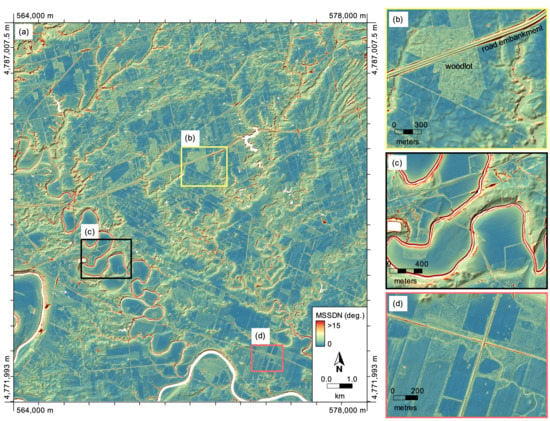
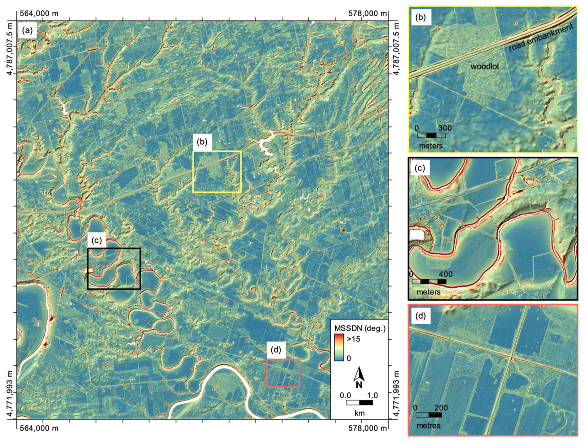
The highest σ
s max values were found to occur along the steep cut banks and terrace scarps of the deeply incised rivers within the site (
Figure 4). By comparison, the wide floodplains and scroll-bars of Fairchild Creek and the Grand River are among the least texturally complex locations within the site, being broadly level, depositional topography. Each of the ravines associated with the smaller incised channels within the northeast of the site demonstrated relatively high roughness, typically peaking at intermediate to broader spatial scales (
Figure 5). Road embankments, and particularly their associated roadside ditches, frequently exhibited high σ
s max values (
Figure 4b). The irregular ground associated with forest floors demonstrated elevated roughness relative to their surrounding agricultural areas; an example of this phenomenon is illustrated in the detailed inset provided in
Figure 4b. The fine texture associated with tillage patterns within agricultural fields were also evident in the σ
s max map, and in fact, the differing tillage direction and furrow depths of neighboring fields, are discernable in the image (
Figure 4d).
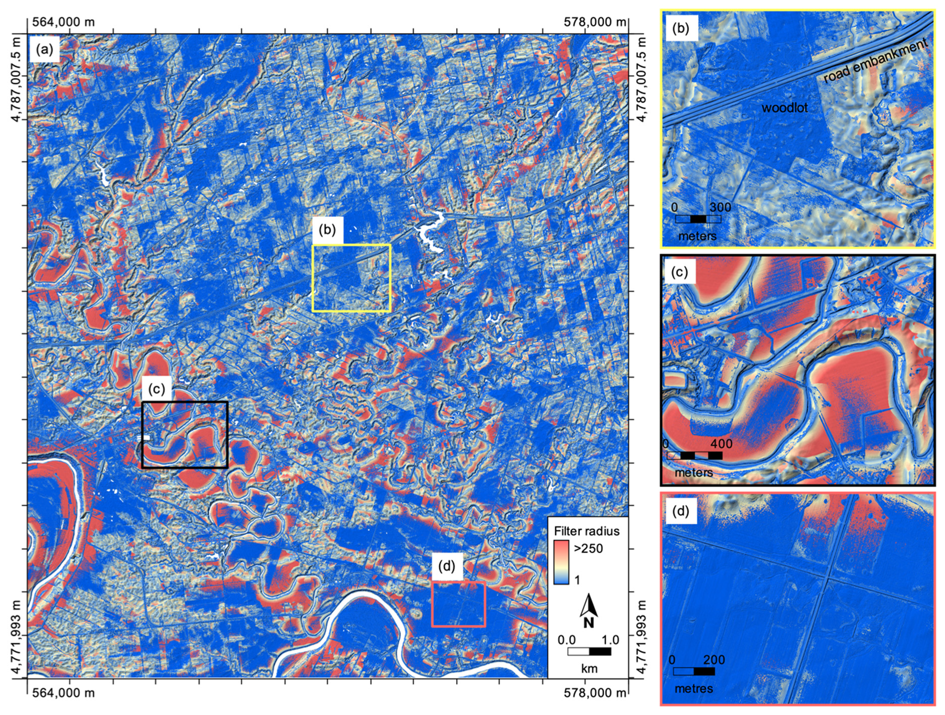
The spatial distribution of
rmax (
Figure 5) illustrated several characteristics about σ
s max. First, flatter agricultural fields containing prominent tillage patterns and forested areas reached peaks in σ
s at shorter scales, typically with 1 ≤
r ≤ 4. These short scales are very extensive in the study site owing to the prevalence of these land covers (
Figure 6). The longest spatial scales of peak σ
s largely coincided with the smooth floodplains on the inside of meander bends (point bars). Fields exhibiting rolling topography possessed more intermediate (20 ≤
r ≤ 70) scales of σ
s max. These scales also coincided with a secondary peak in the probability density function (
Figure 6) located at
r=51 (25.5 m), indicating the prevalence of these roughness scales within the site.
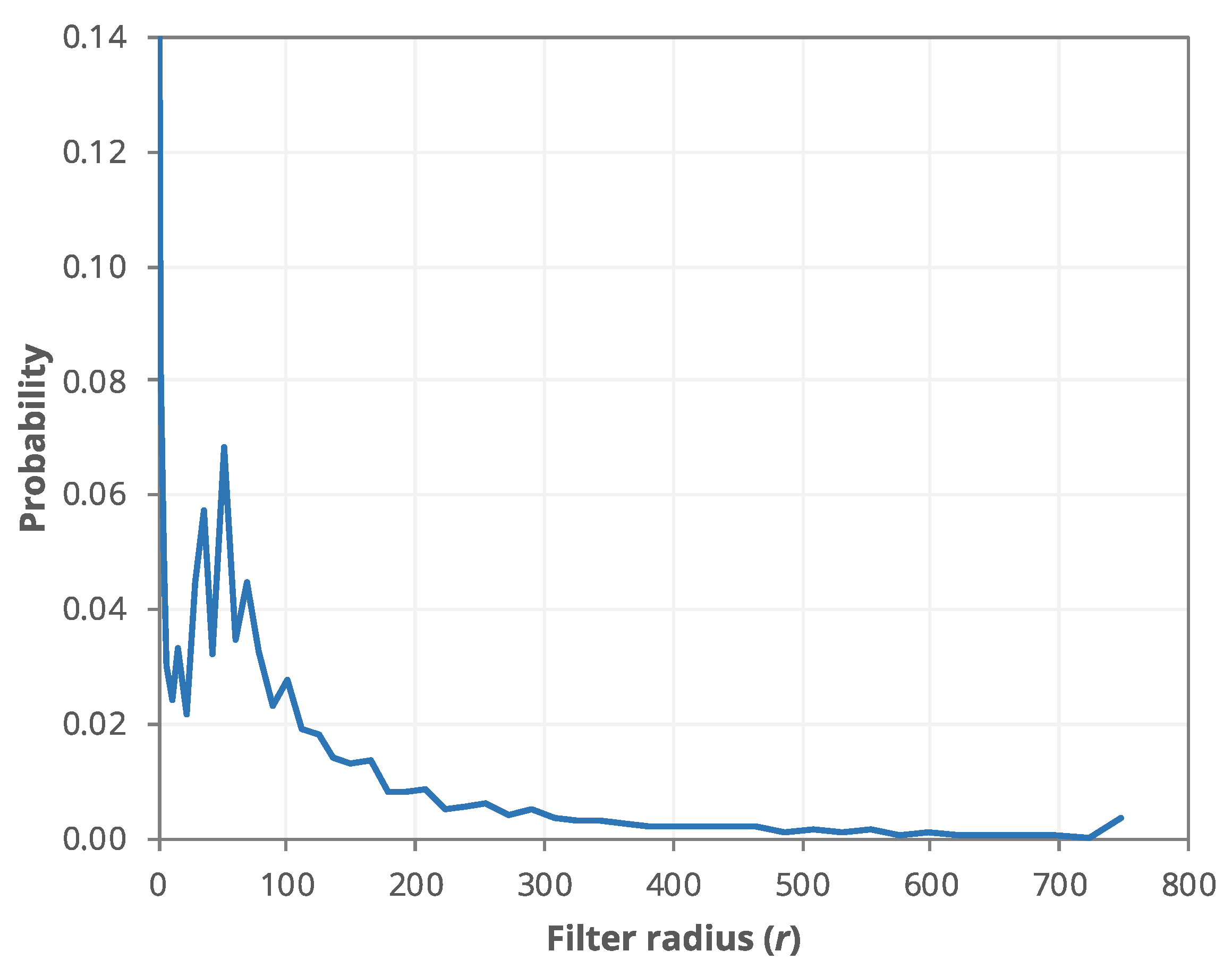
Approximately 35.6% of the grid cells were found to have
rmax values less than four grid cells, indicating the dominance of micro-topographic roughness within the 0.5 m resolution study area DEM. The peak in σ
s values was very rarely identified at filter radii greater than approximately 300 cells (150 m) within the study site and only a small proportion of the grid cells were assigned σ
s max at the tested
rU value (
Figure 6). This would indicate that the
rU value used in this case study (
rU = 748) was sufficient to capture the vast majority of the dominant scales of roughness within the evaluated terrain. The condition of
rmax =
rU may be indicative of a truncated peak in the scale signature at the broadest tested scales. Thus, it is advisable to set the
rU value high enough that only a small proportion of grid cells in the DEM are assigned this upper boundary value. Only 0.36% of the grid cells in the study site DEM were found to have
rmax =
rU (
Figure 6).
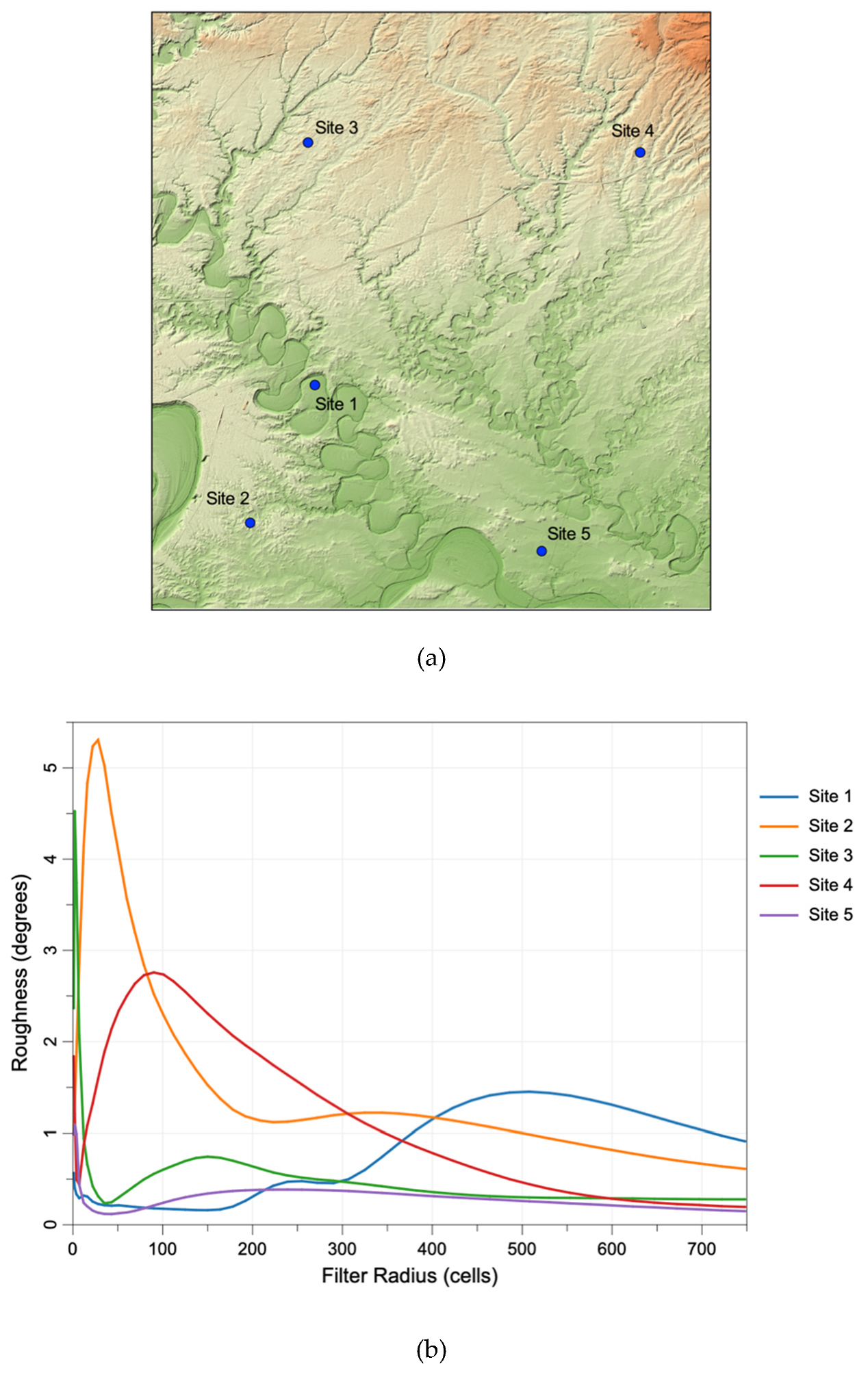
Detailed scale signatures were extracted for five sites within the larger study area, with varying topographic and land-cover characteristics (
Figure 7). Each of the signatures possessed at least one well-defined peak in roughness and demonstrated decreased σ
s variability for scales greater than approximately 500 m. The diversity in overall signature shape and peak location was found to be high. Site 1 was situated on the inside bend of a meander (
Figure 7a) and exhibited generally low σ
s values for
r ≤ 350, peaking at
r = 508 (
Figure 7b). Site 2 was located atop a low hill in an agricultural field typical of the rolling topography found in places throughout the study site. The tillage pattern in the Site 2 field was not as prevalent as in other sites. The site’s signature (
Figure 7b) possessed two peaks; the first and highest peak was located at
r = 28, while the second much lower peak occurred at
r = 344. This first peak was associated with the dimension of the low hill on which the site was situated, while the lower secondary peak was related to a larger-scale topographic undulation within the field. Site 3 was in the middle of a woodlot with a highly irregular forest floor. The first peak in roughness at Site 3 occurred at
r = 2 and was the second highest measured roughness peak of the tested signatures. This peak was associated with the micro-topography of the forest floor, while the secondary peak, situated at
r = 150, resulted from the larger-scale sloping topography of the woodlot. Site 4 was located along a small incised headwater stream, which passed through an agricultural field. The roughness related to the prominent tillage pattern within the field is apparent in the spike in σ
s value at the smallest scales, but the dominant peak in the scale signature occurs at
r = 90 and was caused by the relatively steep hillslopes on either side of the channel. Finally, Site 5 was situated within a flat agricultural field. Unsurprisingly, in the absence of larger-scale topographic features, σ
s max occurs at
r = 1 and reflects the tillage within the field. Roughness was consistently low across all scales for Site 5, although it did exhibit a slight rise in σ
s for the range 50 ≤
r ≤ 239, before gradually dropping again at larger scales (
Figure 7b).
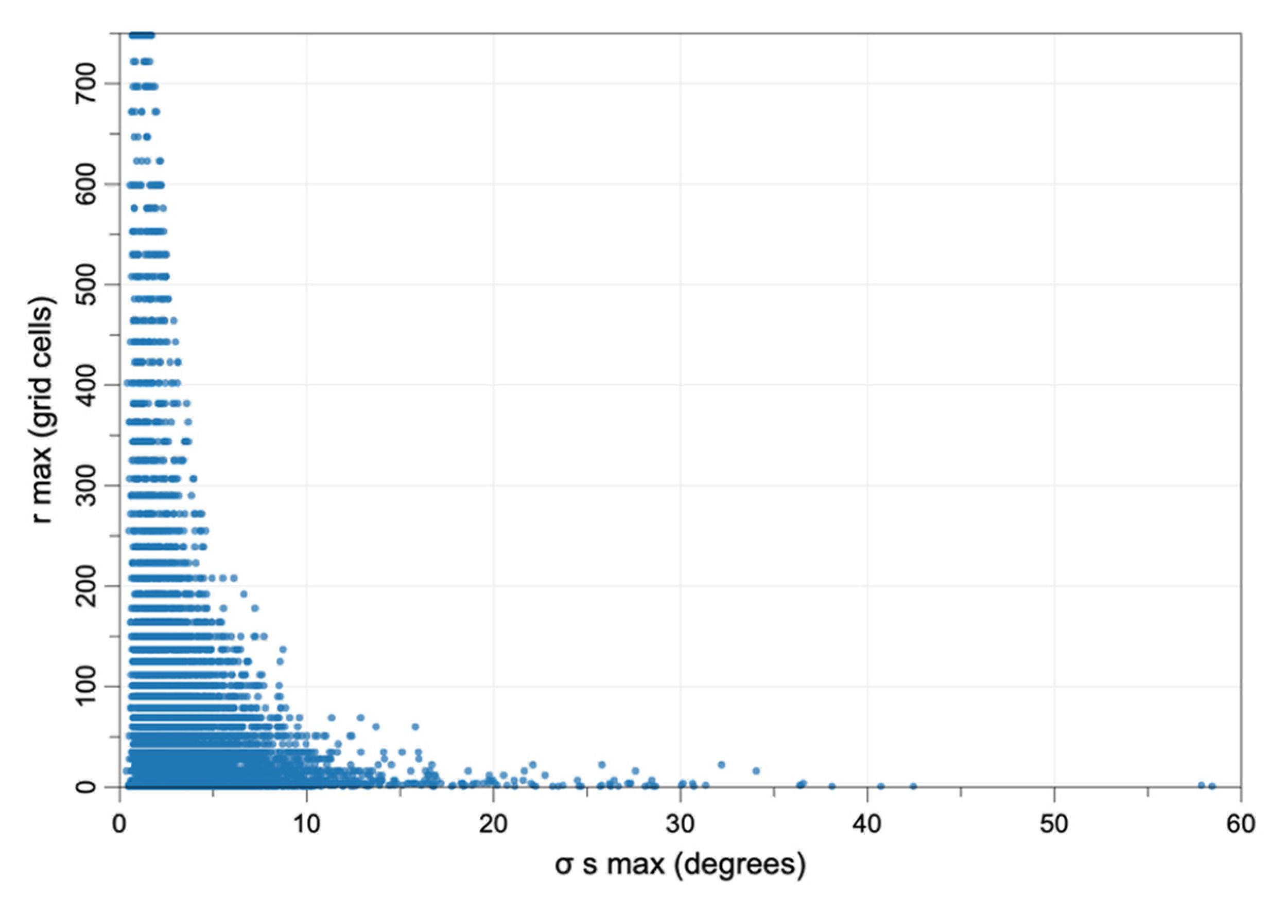
Analysis of the patterns of σ
s max and
rmax revealed negative exponential relation (
Figure 8). This clearly demonstrates the inverse relation between the two indices, such that the grid cells exhibiting the largest σ
s max values (> 20°) are typified by
rmax < ~50, and similarly, that sites with
rmax > 250 exhibit σ
s max < ~ 5°.
A comparison of the summary statistics of σ
s max (
Table 2) and
rmax (
Table 3) distributions was made among the various soil texture categories within the study site. One-way ANOVA testing showed that the soil texture category means were statistically heterogeneous for both σ
s max (F
α = 0.05, df
1 = 8, df
2 = 776,113,757 = 4,597,316.144,
p < 0.0001) and
rmax (F
α = 0.05, df
1 = 8, df
2 = 776,113,757 = 1,560,163.151,
p < 0.0001). Of course, given a sufficiently large sample, extremely small and non-notable differences can be found to be statistically significant and statistical significance says nothing about the practical significance of a difference. Nonetheless, examination of
Table 2 and
Table 3 does reveal noteworthy differences among the distributions of the two roughness indices. For example, silty clay, silty clay loam, and loamy sand each exhibited relatively low average σ
s max while organic soils were notable for their relatively high average σ
s max. Each of the sandy textures appeared to have substantially less range in σ
s max than the other categories. Organic soils exhibited less variability in
rmax values while the median
rmax for silty clay and very fine sandy loam soils were notably lower than other categories. Loam, fine sandy loam, and loamy sand were discernable for their longer mean and median
rmax values. As a whole, the
rmax distributions within each soil category were more skewed (see mean relative to median) than the corresponding σ
s max values.
4. Discussion
The extensive use of integral images and parallelization within the MSSDN tool makes applying this approach to study the hyperscale characteristics of surface roughness in heterogeneous landscapes practical without the need to adjust DEM resolution using resampling or other data coarsening techniques [
4]. The case study shows that it is possible to sample scales densely, even for massive DEMs, allowing for locally optimal scale selection. However, while the approach used in this study was found to be computationally performant, it does require significant memory resources. The large memory requirement of the tool results from the need to store each of the integral images of the three normal vector components with double-precision (64-bits) to avoid rounding errors. Therefore, multi-gigabyte DEMs may not be able to be processed on memory-constrained systems without first splitting the data into smaller pieces. Memory usage issues associated with the application of integral images have been widely recognized in the literature [
27,
28]. This may become less of a restrictive issue as computing platforms with greater memory become more commonly available and as researchers continue to move toward cloud computing platforms, such as Google Earth Engine, for spatial analysis [
29].
Areas of relatively high roughness largely coincided with the smaller incised channels and the cut banks and terrace scarps of larger rivers, as well as road embankments. The impact of road embankments emphasizes the importance of removing these features from fine-resolution LiDAR DEMs in certain applications [
30]. The areas of the study site that were under forest cover were each associated with moderate to high values of roughness. This is indicative of how well the source LiDAR data were able to capture the rough ground beneath the forest canopy, a characteristic of LiDAR data sets that has been previously observed in the literature [
7,
31]. Generally, areas of high roughness were associated with shorter spatial scales and vice versa (
Figure 8), with a relation described by a negative exponential distribution. Some of the longest scales of σ
s max in the site were situated along the broad floodplains and meander scroll-bars, which were also among the least topographically complex (i.e., smoothest) sites. These highly level sites experience maximum roughness at larger spatial scales, such that search windows overlap with the relatively more complex surrounding topography.
The combination of the maximum roughness (
Figure 4) and the scale of maximum roughness (
Figure 5) aided in the interpretation of topographic properties of the study site. While roughness is commonly used as an input parameter for modelling applications, we suggest that the additional information of the scale of peak roughness (
rmax) may provide additional useful information on landscape structure for these applications. The mosaic of spatial scales associated with maximum surface complexity (
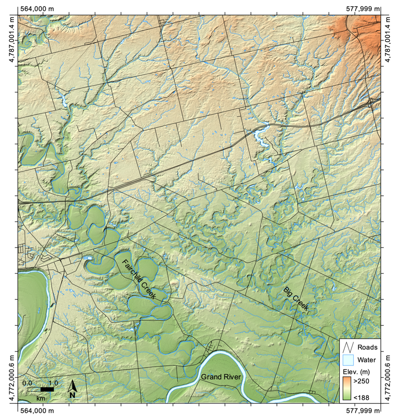
Figure 5) revealed substantial information about the topographic character of the test DEM (
Figure 3) and was demonstrated to be linked with soil texture (
Table 2 and
Table 3). The widely ranging
rmax values show that there is no single ‘representative’ kernel size that can be chosen to characterize topographic texture in a complex and extensive area. As fine-resolution LiDAR DEMs become increasingly common in terrain modelling applications [
32,
33], multiscale analysis of land-surface parameters has become more important [
12,
34,
35] and has the potential for improving the accuracy of mapping and classification applications. Future research should explore the extent to which locally-adaptive scale selection, such as the scheme used in this paper, can also impact geomorphometric mapping and classification applications.
By evaluating this locally-adaptive scale selection method for characterizing roughness (i.e., site-specific scale of maximum roughness) it is evident that the information content in the MSSDN map (
Figure 4) cannot be replicated by the common approaches of 1) measuring roughness at an, often arbitrary, single ‘representative’ scale, or 2) using a stack of roughness maps derived across a range of spatial scales. This last point may not be immediately evident, particularly given the fact that the MSSDN map is itself derived from the multiscale image stack. However, given the heterogeneity observed in the scale signatures among DEM grid cells (e.g.,
Figure 7), in diverse terrain, any classification model that is based on applying weights to each image in a roughness scale stack cannot represent the same information as contained in an MSSDN image. Furthermore, there is potential to extend this approach to derive additional information based on other characteristics of scale signatures, e.g., roughness variability, number of peaks, peak height ratios, etc.
The approach to multiscale roughness analysis used in this research is highly adaptive to different DEM data sets and resolutions, as well as applications. For example, while micro-topographic roughness was found to dominate much of the study area, if the larger-scale surface complexity associated with landform features were of specific interest, it would be possible to remove the impacts of smaller-scale roughness by selecting a larger
rL value. If, instead, an application warrants focusing on surface roughness at shorter scales (e.g., Campbell et al.’s [
36] recent examination of the impact of roughness on human travel through forested terrain), then it would be appropriate to select a relatively low
rU value. It should be possible to similarly apply this technique to study regional-scale roughness patterns at the continental scale using available global DEM products. That is, the lower and upper bounds of the test scales should be suited to the specific application. The use of Gaussian blur to partition roughness scales ensures that roughness is not accumulated from smaller spatial scales to impact the interpretation of features at a larger scale.


