Article

Earthquake-Induced Landslide Risk Assessment: An Example from Sakhalin Island, Russia

Sakhalin Department of Far East Geological Institute, Far Eastern Branch, Russian Academy of Sciences, Yuzhno-Sakhalinsk 693023, Russia
*
Author to whom correspondence should be addressed.
Geosciences 2019, 9(7), 305; https://doi.org/10.3390/geosciences9070305
Submission received: 30 April 2019 / Revised: 4 July 2019 / Accepted: 8 July 2019 / Published: 11 July 2019

Abstract

:
Damages caused by earthquake-induced ground effects can be of the order or significantly exceed the expected damages from ground shaking. A new probabilistic technique is considered in this study for earthquake-induced landslide risk assessment. A fully probabilistic technique suggests a multi-stage hazard assessment. These stages include the determination of seismic hazard curves and landslide probabilistic models, a vulnerability assessment, and geotechnical investigations. At each of the stages, the uncertainties should be carefully analyzed. A logic tree technique, which handles all available models and parameters, was used in the study. The method was applied considering child education facilities located at the foot of a natural slope in the south of Sakhalin Island which is known as an active seismic and land sliding area. The significant differences in the ground motion scenario in terms of the 475-year seismic hazard map and the fully probabilistic approach considered suggests that seismic landslide risk could be underestimated or overestimated when using the 475-year seismic hazard map for risk assessment. The given approach follows the rational risk management idea that handles well all possible ground motion scenarios, slope models, and parameters. The authors suggest that the given approach can improve geotechnical studies of slope stability.

1. Introduction

Large earthquakes affecting urban areas are one of the most destructive natural hazards and can lead to significant impacts on the built and human environment. Generally, earthquake loss models consider ground shaking and ground failure (such as landslides, liquefaction, and faulting) hazards. Damages caused by earthquake-induced ground effects, in some cases, significantly exceed the damages from direct ground shaking [1,2]. Damages related to seismically-induced landslides can be considerable due to the full collapse or loss in functionality of facilities, roads, pipelines, and other lifelines [3,4,5,6,7].
There are numerous causative factors for seismically-induced gravity-slope processes on Sakhalin Island, which is recognized as an area with a high level of geohazards. A total of 70% of the South Sakhalin territory is susceptible to landslide activity [8]. According to general seismic hazard maps, Sakhalin Island is a seismically active area, with an 8–9 MSK-64 macroseismic intensity for the 475-year return period [9].
As a recent example of earthquake-induced landslides, the Mw = 6.2 2 August 2007 Nevelsk earthquake should be noted. The Nevelsk earthquake was followed by aftershock sequences with a relatively high productivity level [10]. Focal mechanisms of the mainshock and aftershocks indicates the west dipping (38–40°) fault planes.
The largest aftershock with a magnitude of Mw = 5.9 followed about two hours after the mainshock origin time. They generated tsunami waves up to 3.2 m high. The ground shaking effects in Nevelsk caused by the mainshock and largest aftershock corresponded to a 7–8 MSK-64 macroseismic intensity (Figure 1). Massive damages of buildings (>200), bridges, railway and roads were found during macroseismic inspection [10].
The 2007 Nevelsk earthquakes caused massive release of methane from the coal beds in the coastal zone of 40 km in length and an uplift of benches in the area of the Nevelsk sea port [10].
As a result of significant ground shaking, subsidence cracks and shallow landslides (up to 200–300 m3) were widely recorded (Figure 2) within the Nevelsk urban area (16–21 km from the epicenter). The 2007 Nevelsk earthquake occurred in a relatively dry period. There was a recorded 69 mm of rain precipitation, representing 45% of the mean annual value, for the two months before the mainshock [11]. Therefore, seismically-induced landslides remain a major natural hazard on Sakhalin Island that should be considered in the risk assessment strategy.
Most hazard assessment techniques are designed for producing susceptibility or likelihood maps on large scales (regional or global) [2,12,13]. Because material parameters are difficult to identify in detail for large areas, slope parameters are estimated from topographic, geologic, and other geospatial information. These maps are most commonly used for an estimation of the general hazard level and specifying sites where detailed geotechnical investigations are needed.
The aim of this study is to apply the earthquake-induced landslide risk assessment technique at a local scale. This paper proposes a fully probabilistic approach that handles all available ground motion scenarios and geomechanical slope models well. The important issue is the estimation of the uncertainties from the spatial and temporal variability of soil parameters.
The child education facilities (Figure 3) located under the natural slope in Nevelsk (Sakhalin Island, Russia) were considered in this study as an example of the given approach. This site was proposed for application of the methodology due to available slope material parameters previously obtained from geotechnical investigations.

2. Materials and Methods

2.1. Fully Probabilistic Risk Assessment Technique

The seismic hazard maps in terms of the 475-year ground shaking intensity are most commonly used as a triggering condition for analyzing the slope stability under seismic loading [2,13,14]. Uncertainties about the ‘best’ ground motion scenario for land sliding prediction are still being discussed [15].
A fully probabilistic risk assessment technique that handles all available ground motion scenarios well is considered in this study [16]. The given approach follows a rational risk management idea that deals with all possible models, scenarios, and uncertainties.
The total risk of an earthquake-induced landslide hazard to the facility located at the foot of the slope in the next T years can be expressed in terms of probability and vulnerability. Formally, the probability of the occurrence of N seismically-induced landslides within a certain time interval should be considered. In practice, the probability of the triggering of two or more slope failures within 50 years is extremally small.
A fully probabilistic approach suggests determination of the occurrence probabilities of various ground shaking levels and probabilities of landslide triggering for these ground motion scenarios. That gives the total probability of earthquake-induced slope failure in a certain time interval considering all possible ground motion scenarios:
P s f ( T ) = j i w j P ( PGA = a i | T ) · P r j ( a i ) = j i w j p i j ,
where P ( PGA = a i | T ) is the probability of the occurrence of ground shaking level a i in the next T years (ground motion scenario), P r j ( a i ) is the probability that seismic loading a i will trigger a landslide in the frame of the geomechanical slope model j , p i j is the probability of slope failure in the next T years under ground motion scenario a i in the frame of the geomechanical slope model j , and PGA is the peak ground acceleration at the given site.
The summation in (1) is carried out for all available geomechanical slope models ranked by weights w j , where:
j w j = 1 .
The resistance of the facility to prevent the land sliding can be expressed in terms of the structural damage risk (physical vulnerability). The vulnerability is defined in this study as the degree of loss of a given element at risk and ranging from 0 (no loss) to 1 (total loss).
Vulnerability depends on a number of factors [17,18], such as the sliding mass volume and its velocity, position of landslide initiation, etc. For an accurate risk assessment, all of these factors should be considered. In many case studies, the vulnerability assessment is still characterized by large uncertainties.
In a simple case, vulnerability depends on the intensity of the landslide that can hit the facility located at some distance from the landslide source [18,19]. It means that a certain geomechanical slope model can be associated with the expected intensity level of the landslide.
Then, the total risk R ( T ) of facility damage caused by seismic land sliding within T years can be written as:
R ( T ) = j i w j v j p i j ,
where v j is the vulnerability of the facility in the frame of the geomechanical slope model j .
Basically, Equations (1) and (3) suggest a multi-stage and multi-hazard approach. These stages include site-specific probabilistic seismic hazard analysis, vulnerability assessment, geotechnical investigations, and landslide probability calibration.

2.2. Causative Factors of Studied Area

Seismically-induced landslide risk assessment is complicated by the numerous factors and conditions contributing to slope failure. This section discusses the major causative factors of the studied area, helping to constrain the slope models and parameters for the probabilistic hazard analysis (Figure 4).

2.2.1. Geology

From the basis of the tectonic terrains scheme, the studied area is related to the southern part of the West Sakhalin Terrane located to the north of the Lopatino Cape. The target area consists of Late Cretaceous and Cenozoic outcropping rocks (Figure 5).
Quaternary and Neogene age deposits are widely presented in the studied area. The Quaternary soils of low-thickness are presented by deluvial-eluvial deposits. The Neogene soils of the Nevelskaya formation are presented by volcanic sandstones, siltstones, tuffs, and tuffits. A geologic map with detailed formation lithology is given in Figure 5 [20].
From the view of general engineering geology, the following layers are highlighted in the lithological slope section: 1—topsoil (0.2 m); 2—fine-gravelly with sandy filler up to 50%, dense (deluvial-eluvial) (0.2 m); 3—tuff-sandstone on clayey cement with low-strength siltstone interlayers (3.6 m).

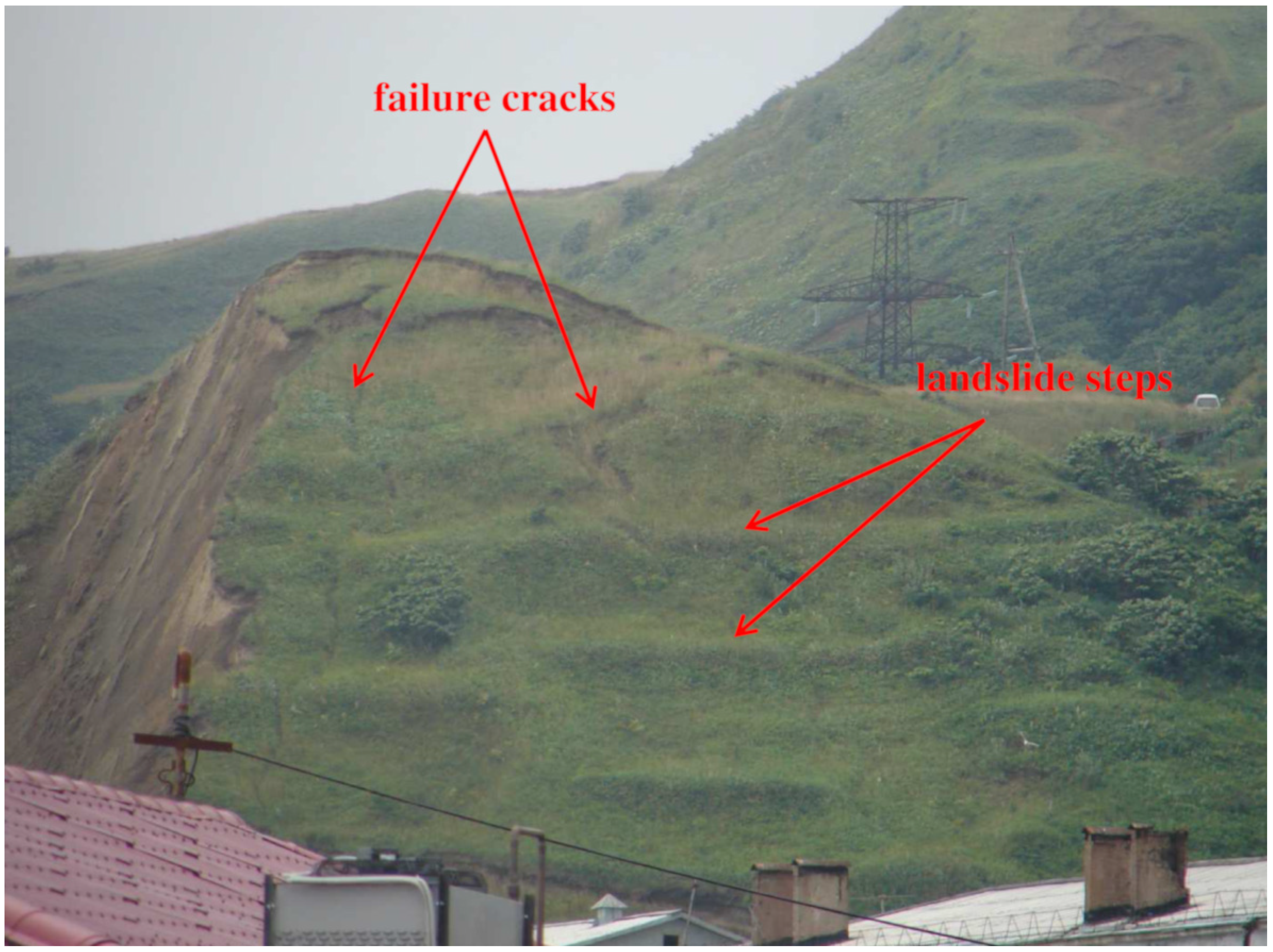
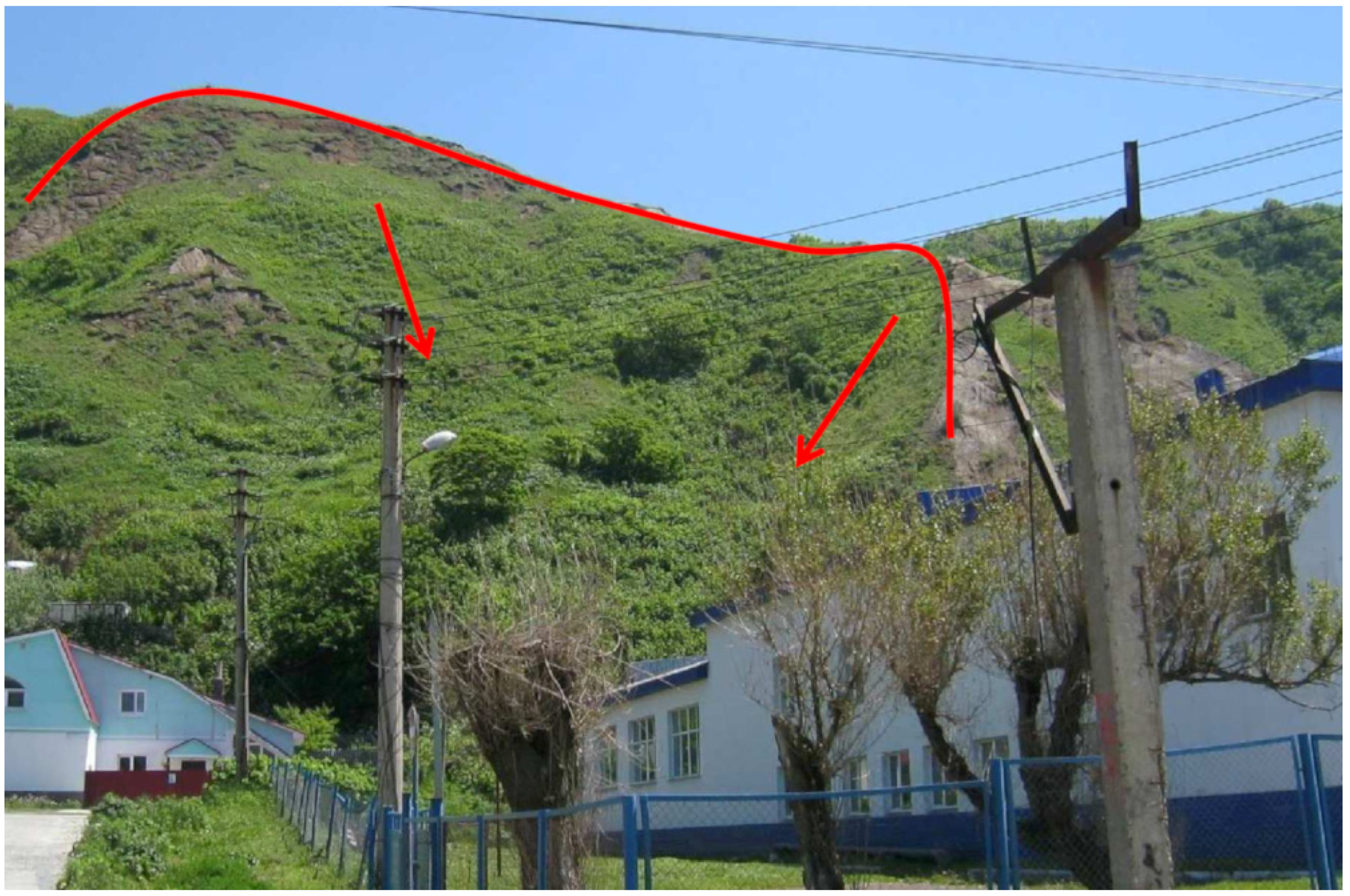
2.2.2. Geomorphology

Nevelsk is located on the western flanks and sea terrace’s foot, which are western branches of the South Kamyshoviy range. Terraces have an absolute elevation till 200 m and are dissected by narrow, deeply incised V-shaped valleys of rivers and rills [21].
Landscape dissection depth reaches 200 m, and the slope steepness is 45° and more. Terrace surfaces are inclined to the sea side.
Abrasion sea terrace scarps, rivers, and rill valley slopes are well-sodded and covered by grassy-shrub vegetation, and in some places are forested. Vegetation does not prevent landslides.
River valley and sea terrace slopes are complicated by old block slides, which make slopes stepped.
The child education facilities are located close to the foot of the high sea terrace (Figure 3 and Figure 4).

2.2.3. Climatic Settings

The Nevelsk district is located along the Tatar Strait of the Japanese Sea, and is strongly affected by a warm Tsushima current, so it witnesses the warmest summer and winter of the entire island. The territory is characterized by a large precipitation quantity during the second part of the summer.
The mean annual precipitation quantity in Nevelsk is 911 mm [22]. Precipitation falls inhomogenously. The major precipitation period is related to the second half of the summer and early autumn, and the minimum period is the second half of winter.
Two landslide activation periods related to soil moisture conditions are typical for the studied area.
The first period (end of May to early June) is related to melting snow which leads to rapid soil humidification and often, to shallow (1 m deep) landslides. Rainfall can trigger landslides during this period.
The second period (August to October) is related to high cyclone activity, leading to a large rain precipitation quantity.
The long-term annual average precipitation quantity during the warm period is 579 mm. The rainiest month is September, with a precipitation quantity of ~111 mm. The precipitation quantity during a cyclone event (in August–September) can exceed the monthly average level. The maximum precipitation quantity (211 mm) was registered during the Phillis cyclone event (2–7 August 1981).

2.2.4. Soil Moisture Conditions

The soil moisture conditions of a potentially sliding mass represent one of the most important factors for landslide prediction.
Three soil moisture models are assumed. The models are constrained by generalizing the climatic settings in the studied area. These simplified models are characterized by the following properties:
  • Slightly wet—Shallow invasion of the water into the soil mass. Dry soil conditions are typical for drought periods and for periods with stable snow cover. The overall period duration is about five months;
  • Moist—Invasion of the water into the soil mass to a 1 m depth. The overall period duration is three months;
  • Water saturated—Soil mass is waterlogged to a ~2 m depth. This model is typical for the rain precipitation and rapid snow melting coincidence period and for cyclone/typhoon occurrences. The overall period duration is about four months.

2.3. Materials

2.3.1. Ground Motion Scenarios

The main goal of probabilistic seismic hazard analysis (PSHA) is to determine the probability of exceeding a certain ground shaking level at a given site within the time interval of interest [23]. The result of such analysis is a seismic hazard curve, which demonstrates the relationship between the probability of exceeding P ( PGA > a | T ) and ground shaking level a . Under ground shaking conditions, we consider PGA.
The occurrence probability P ( PGA = a i | T ) is recognized in this study as a ground motion scenario. The transition from the probability of exceeding to the discrete probability is given as:
P ( PGA = a i | T ) = P ( PGA > a i | T ) P ( PGA > a i + 1 | T ) .
Therefore, Equation (4) defines the probability of the occurrence of a certain ground shaking level in the next T years. It was substituted into Equations (1) and (3).
The seismic hazard curve for a given site was computed using CRISIS 2015 software [24]. The authors used the regional seismic source models and ground motion prediction equations tested in the previous PSHA studies [25].
The average 30-m ground layer shear-wave velocity VS30 at the site is of the order of 300 m/s. It was used for site correction within the PSHA stage considering the site-correction term in the ground motion prediction equations.
The seismic hazard curve used in this study is shown in Figure 6. The 10% exceeding probability (or 475-year return period probability) corresponds to the PGA value of 0.38 g (Figure 6). Peak ground acceleration of 0.38 g corresponds to a ground shaking intensity of 9 MSK64. It is in good agreement with the estimates based on the maps of general seismic zonation [9].

2.3.2. Probability of Landslide Triggering

Jibson et al. [12] calibrated the slope failure probability by analyzing landslide field data after the 1994 Northridge earthquake and predicted Newmark displacement ( D N ). The authors used the Newmark sliding block model [26] to quantify the probability of landslide triggering given the PGA value ( a ) and critical slope acceleration ( a c ). The Jibson probability model follows the Weibull distribution:
P r ( D N ) = 0.335 [ 1 exp ( 0.048 D N 1.565 ) ] ,
where
log D N ( a ) = 0.215 + log [ ( 1 a c a ) 2.341 ( a c a ) 1.438 ] ± 0.51 .
The critical slope acceleration a c of a sliding mass is considered as a simple function of the static factor of safety F S and the slope geometry:
a c = ( F S 1 ) g sin α ,
where g is the gravity factor and α is the dip angle of the potential sliding surface.
According to the limit equilibrium theory, the static factor of safety F S is defined as the relationship between the force keeping the sliding mass on the slope and the force moving the sliding mass down the slope [12]:
F S = c γ z sin α + tan φ tan α m γ w tan φ γ tan α ,
where c is the effective cohesion, z is the slope-normal thickness of the potential sliding mass, γ is the material unit weight, γ w is the unit weight of ground water, φ is the effective friction angle, and m represents the fractional depth of the water table with respect to the total slide depth. The sliding mass is stable if F S > 1 , and unstable when F S < 1 .
Soil moisture conditions in the studied area and southern California are significantly different. Virtually no rain had fallen prior to the 1994 Northridge earthquake, which was used for calibrating the seismically-induced landslide probability [12]. The pore-water pressure term was dropped from Equation (8) in the Jibson probability model. The soils in the studied area are expected to be saturated most of the year, so the authors paid great attention to the third term of Equation (8). Several models with a non-zero pore-water pressure term are hypothesized in this study.
Therefore, the Jibson probabilistic model for California (5) was imported into the Equations (1) and (3).

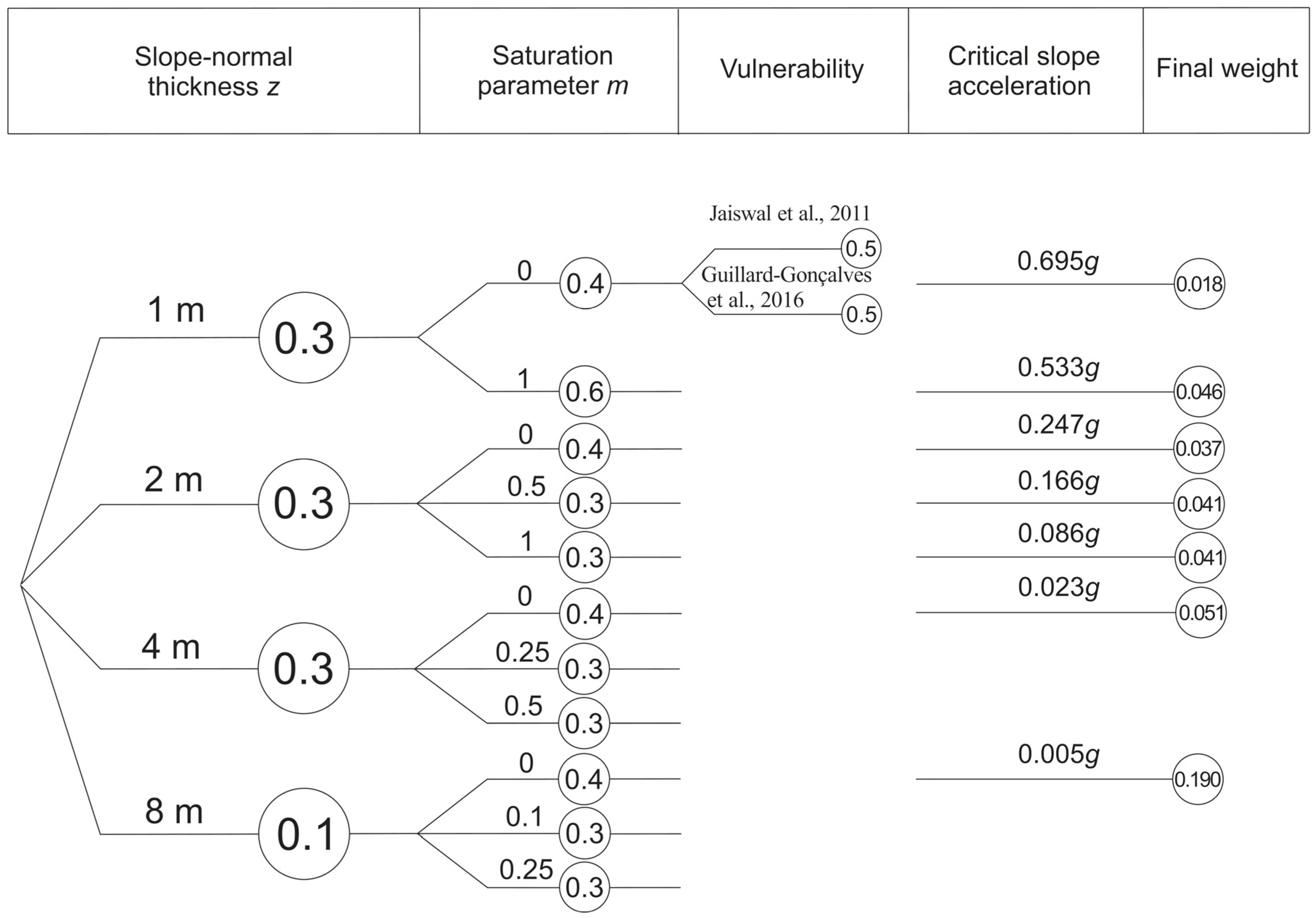
2.3.3. Geomechanical Slope Models and Logic Tree

The physico-mechanical parameters of the slope soils were obtained during geotechnical investigations at the site (see Acknowledgments Section). Geotechnical studies included sampling undisturbed cores and laboratory tests. The material parameters of the soil mass are given in Table 1.
Identifying the slab thickness z of potential sliding mass requires high-quality seismic profile, geological, and geophysical data. These can give additional information about the layer structure that helps to fix the slope-normal thickness or to identify the preexisting landslides. Such data is not available for the studied area. Therefore, the slab thickness variability was hypothesized through the logic tree approach, which is commonly used in PSHA. Four models with varied slab thicknesses (1, 2, 4, and 8 m) were considered. The corresponding weights are equal to 0.3, 0.3, 0.3, and 0.1 (Figure 7). The weights were determined by an expert’s view.
The given difference in weighting reflects our view that the landslide initiation depth of an order of 8 m seems to be unrealistic. However, the authors are aware of the uncertainties connected with this choice in weighting scheme.
The accurate weighting of models with slab thickness uncertainties can be realized through the corresponding probability density distribution. The probability that the landslide has a certain slip surface depth value is defined by its statistical distribution. A significant amount of observations in the studied area are required for developing such a probability model.
The second variable parameter is the proportion of the sliding mass thickness that is saturated ( m in Equation (8)). The water saturation parameter was defined as a simplified relation given by soil moisture conditions (see Section 2.2.4):
m = depth   of   water   invasion slab - normal   thickness .
The proportion between the period duration of water invasion into the corresponding soil depth and the annual period was used for the weighting. For instance, for dry soil conditions, the corresponding weight was defined as 5/12~0.4 (Figure 7).
A full logic tree that handles uncertainties in the considered models and parameters is shown in Figure 6. The resulting critical slope acceleration for each branch was calculated according to (7). For the unstable case ( F S < 1 ), the critical slope acceleration was defined as the minimum acceleration in the given seismic hazard curve (0.005 g).

2.3.4. Vulnerability Assessment

The physical vulnerability term is widely used in many scientific and engineering fields [27]. It defines the probability that a given element at risk will be damaged under a certain impact. Recent seismic risk analyses have usually dealt with seismic fragility curves [28]. The fragility curve defines the conditional probability of exceeding the certain damage state of the building for a given level of ground shaking intensity. Increasing the research volume of earthquake damage data allows researchers to calibrate seismic fragility curves in many seismically-active regions.
Unfortunately, accurate calibrating of the fragility curves is still complicated by limited damage data for most types of landslides. Moreover, different physical mechanisms are associated with different types of landslides (rockfalls, block slides, debris flow etc.). Vulnerability depends on a number of factors [17,18], such as the sliding mass volume, landslide velocity, landslide source, etc.
A physical vulnerability assessment is characterized by uncertainties that can be either epistemic or aleatory [29]. Epistemic uncertainties can be associated with the simplification of the landslide intensity estimation, the characterization of elements at risk, the vulnerability models, expert view, etc. Aleatory uncertainties can be associated with the spatial variability of parameters [29], such as landslide source location. For this type of uncertainty, the expected structural damage differs, depending on whether the facility is located on the foot or landslide body [19].
Russian regulation norms have a specific definition of landslide hazard, depending on its type and volume, but quantitative estimations of the structural response are not available.
Due to the reasons mentioned above, vulnerability assessment still remains somewhat subjective and is usually performed in small study areas (local scale). The main issue of the vulnerability assessment in our study is to give a suitable estimation of expected damage using different sliding mass models.
Available data that defines the physical loss of buildings for the wide range of sliding processes were used in this study [18,19]. Most available data for physical damage estimates come from debris flow studies. However, the authors are aware of the uncertainties connected with the choice of vulnerability values.
Different vulnerability values in connection to the expected intensity level of a landslide and facility type are given in [18]. Jaiswal et al. [18] used the landslide volume for intensity estimation (M-I, M-II and M-III). The M-I intensity class corresponds to shallow landslides with a volume of less than 1000 m3. If a landslide becomes bigger, with a volume ranging from 1000 m3 to 10,000 m3, the intensity follows the M-II class. For landslides with a volume greater than 10,000 m3, the intensity reaches the M-III class.
For similarity, the landslide volume was estimated as V = A L × z , where A L is the sliding area. The equation A L = min ( 706 × z , A L m a x ) links the normal slope thickness and sliding area [19]. According to field studies, the maximum expected sliding area A L m a x is of the order of 2335 m2 (Figure 3). Despite the fact that the given relationships have significant uncertainties, they help to constrain the landslide intensity class in the studied area.
According to [19], the landslide intensity is associated with the slip surface depth, which is directly related to the slab thickness of the sliding mass. There are [12] five different landslide intensity classes that correspond to the given slip surface depths of 1 m, 2 m, 6 m, 10 m, and 20 m. The estimated vulnerabilities for slip surface depths of 1 m, 2 m, 6 m, and 10 m were imported to our model with corresponding slab thicknesses of 1 m, 2 m, 4 m, and 8 m.
The reinforced concrete building type (Type-4 or SBT4) was used in this study for the vulnerability assessment. This building type is closely related to the child education facilities considered by its material strength properties.
The vulnerability exhibits average, minimum, and maximum values. For dry soil conditions, we use average vulnerability values, and for water-saturated soil conditions, we use maximum vulnerability values, as we expect that a water-saturated sliding mass has a relatively higher landslide velocity.
We used the estimated vulnerability of elements at risk located within run-out paths of a landslide. Table 2 contains the vulnerability estimations for the considered facilitates and slope models in full accordance with [18,19]. The final weights for each of the considered slope models in Figure 6 are given with respect to the vulnerability values from Table 2.

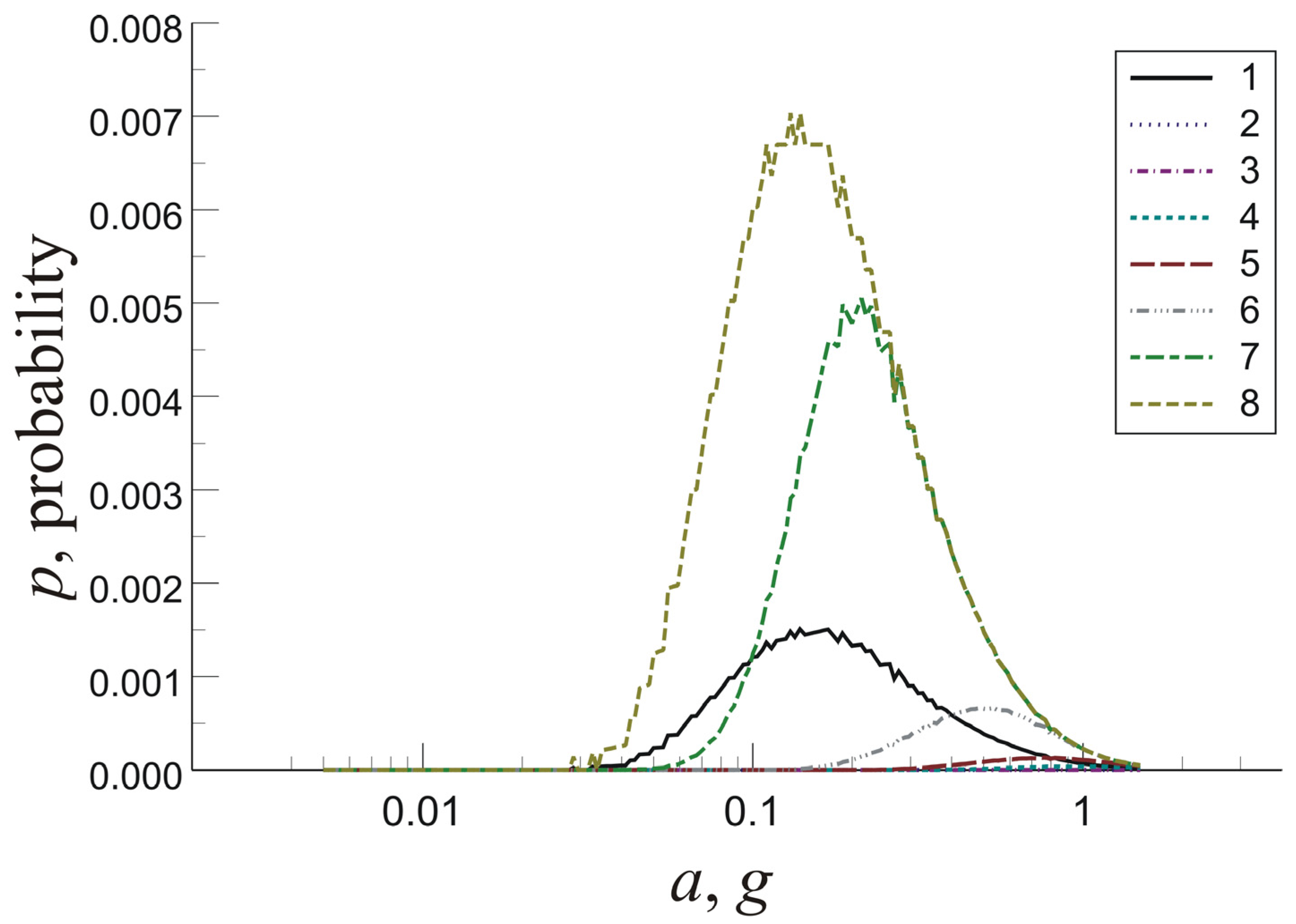
3. Results and Discussion

Since the critical slope acceleration becomes available for each of the considered slope models, it is substituted into the Jibson probabilistic model (4). Next, the probability of occurrence of a landslide ( P r ( D N ( a i ) ) ) under the given seismic loading is multiplied by the probability of the occurrence a certain ground shaking level in the next 50 years ( P ( PGA = a i | T ) ). This gives the probability ( p i j ) of slope failure in the next 50 years under ground motion scenario a i in the frame of the geomechanical slope model j . Then, the summation of discrete probabilities p i j is carried out for all available ground motion scenarios a i and geomechanical slope models ranked by weights w j . Since the final weights for each of the considered slope model are calculated with respect to the vulnerability (Figure 7), the summation of p i j multiplied by its final weights w j gives the total risk value.
The total risk of an earthquake-induced landslide hazard for the child education facility located at the foot of the slope within the next 50 years was computed according to Equation (3) and the weighting scheme illustrated in Figure 7. The corresponding risk value appeared to be 7.4%. It reflects the high level of seismic and landslide hazards and high vulnerability value for the facilities located at the foot of the natural slope. Therefore, the high risk value shows a considerable hazard of seismically-induced landslides in terms of civil engineering.
In order to estimate the most probable ground motion scenario that will cause damage to the facility by an earthquake-induced landslide, the discrete probabilities p i j from Equation (3) were plotted against the corresponding ground motion level. This gives the contribution to the total risk from each slope model and each ground shaking level (Figure 8). As can be seen from Figure 8, the distributions have a modal form.
The average weighted probability density function computed according to the logic tree scheme (Figure 7) has a peak at PGA = 0.15 g (7–8 MSK64 intensity level). The PGA value of the order of 0.15 g can be recognized as the ‘best’ ground motion scenario for the considered slope models and parameters. In terms of PSHA, the given ground shaking level is closely related to the 100-year return period (according to Figure 6).
At the same time, Figure 7 shows the contribution to the total risk from each slope model. The saturated soil’s model (ac = 0.005 plot in Figure 8) should be considered as the most probable scenario for the considered area. Generally, it makes the slope unstable, regardless of the triggering conditions.
The slope model corresponding to the slip surface depth of z = 4 m and dry soil conditions (m = 0) has a clear peak around PGA = 0.2–0.3 g (ac = 0.023 g plot in Figure 8). This ground shaking value is closely related to the 475-year probability.
It should be noted that a significant ground shaking level corresponding to a 7–8 MSK-64 intensity caused shallow landslides within the Nevelsk urban area in 2007. The PGA value corresponding to the ‘best’ ground motion scenario is the same order as the ground shaking intensity in the studied area generated by the 2007 Nevelsk earthquake. No facilities were damaged by the earthquake-induced landslide. This may be explained in terms of soil moisture conditions. The point is that several months prior to the Mw = 6.2 2 August 2007 Nevelsk earthquake, no rain had fallen. As a result, the 2007 Nevelsk earthquakes occurred in a relatively dry period. For such untypical conditions, the corresponding ground motion scenario is the order of PGA = 0.2–0.3 g or an 8–9 MSK64 intensity.
When generalizing results of the study, several assumptions and models should be mentioned.
Constants of the Jibson landslide probability model in the target area are generally not the same as those in southern California. The shape of the probability curve depends on the geological, geomorphological, and soil moisture conditions. Jibson et al. [12] argue that the variability of constants in Equation (4) should be proposed if a significant difference between the target area and southern California is found. This means that the logic tree will be complicated by uncertainties from the landslide probability model.
One more source of epistemic uncertainty comes from the spatial and seasonal variability of slope material parameters. Geotechnical studies of rocks and soils within the large area of the natural slope within different seasons should significantly reduce the uncertainties associated with the variability of geomechanical slope models (Figure 8).

4. Conclusions

A fully probabilistic technique is considered in this study for an earthquake-induced landslide risk assessment in a relatively small area. The given method suggests a multi-stage and multi-hazard approach. These stages include a site-specific probabilistic seismic hazard analysis, vulnerability assessment, geotechnical investigations, and landslide probability calibration.
As a case study, the child education facility located under the natural slope was considered in this study. The total risk of earthquake-induced landslide hazard to the child education facility located at the foot of the slope within the next 50 years was of the order of 7.4%.
A significant difference between the ground motion scenario in terms of the 475-year seismic hazard map and considered fully probabilistic approach suggests that seismic landslide risk could be underestimated or overestimated when using the 475-year seismic hazard map for landslide risk assessment. The given approach follows the rational risk management idea that handles well all possible ground motion scenarios and geomechanical slope models.
An important factor that leads to an increase of the total risk is the saturated soil mass. Geotechnical studies of rocks and soils within large areas of a natural slope within different seasons should significantly reduce the uncertainties associated with the variability of geomechanical slope models.
The aim of future research is to produce regional seismically-induced landslide hazard maps using the fully probabilistic approach.

Author Contributions

Conceptualization, A.K.; methodology, A.K.; software, A.S.; validation, A.S.; formal analysis, Y.G.; investigation, Y.G., V.L., A.M., Y.S., L.M., A.S. and M.M.; resources, A.K. and Y.S.; writing—review and editing, A.K. and L.M.; visualization, Y.S. and A.M.; project administration, A.K. and Y.G.

Acknowledgments

This study was supported through computational resources provided by the Shared Facility Center “Data Center of FEB RAS” (Khabarovsk) [30]. Material parameters of the studied area were supported by Biolit LLC (Yuzhno-Sakhalinsk).

Conflicts of Interest

The authors declare no conflict of interest.

References

  1. Mohammad, E.; Babak, O.; Mahdi, M.; Mohammad, A.N.; Ali, A.A. Sensitivity analysis in seismic loss estimation of urban infrastructures. Geomat. Nat. Hazards Risk 2018, 9, 624–644. [Google Scholar] [Green Version]
  2. Martino, S.; Battaglia, S.; Delgado, J.; Esposito, C.; Martini, G.; Missori, C. Probabilistic Approach to Provide Scenarios of Earthquake-Induced Slope Failures (PARSIFAL) Applied to the Alcoy Basin (South Spain). Geosciences 2018, 8, 57. [Google Scholar] [CrossRef]
  3. Forte, G.; Fabbrocino, S.; de Magistris, F.S.; Silvestri, F.; Fabbrocino, G. Earthquake Triggered Landslides: The Case Study of a Roadway Network in Molise Region (Italy). In Engineering Geology for Society and Territory; Springer: Cham, Switzerland, 2015; Volume 2, pp. 765–768. [Google Scholar]
  4. Keefer, D.K. Statistical analysis of an earthquake-induced landslide distribution—The 1989 Loma Prieta, California event. Eng. Geol. 2000, 58, 231–249. [Google Scholar] [CrossRef]
  5. Xu, C.; Xu, X.; Yao, X.; Dai, F. Three (nearly) complete inventories of landslides triggered by the May 12, 2008 Wenchuan Mw 7.9 earthquake of China and their spatial distribution statistical analysis. Landslides 2014, 11, 441–461. [Google Scholar] [CrossRef]
  6. Esposito, E.; Guerrieri, L.; Porfido, S.; Vittori, E.; Blumetti, A.M.; Comerci, V.; Michetti, A.M.; Serva, L. Landslides induced by historical and recent earthquakes in Central-Southern Apennines (Italy): A tool for intensity assessment and seismic hazard. Landslide Sci. Pract. 2013, 295–303. [Google Scholar]
  7. Porfido, S.; Esposito, E.; Spiga, E.; Sacchi, M.; Molisso, F.; Mazzola, S. Impact of ground effects for an appropriate mitigation strategy in seismic area: The example of Guatemala 1976 earthquake. In Engineering Geology for Society and Territory; Springer: Cham, Switzerland, 2015; Volume 2, pp. 703–708. [Google Scholar]
  8. Lobkina, V.A.; Kazakova, E.N.; Zhiruev, S.P.; Kazakov, N.A. Methods of landslide risk assessment for territory of settlements of Sakhalin Region (Makarov city, Sakhalin). Russ. J. Pac. Geol. 2013, 32, 100–109. (In Russian) [Google Scholar]
  9. Ulomov, V.I.; Bogdanov, M.I. Explanatory note on the GSZ-2016 maps set of general seismic zoning of the Russian Federation territory. Eng. Surv. 2016, 7, 49–122. (In Russian) [Google Scholar]
  10. Konovalov, A.V.; Nagornykh, T.V.; Safonov, D.A.; Lomtev, V.L. Nevelsk earthquakes of August 2, 2007 and seismic setting in the southeastern margin of Sakhalin Island. Russ. J. Pac. Geol. 2015, 9, 451–466. [Google Scholar] [CrossRef]
  11. Reliable Prognosis. Available online: https://rp5.ru/%D0%90%D1%80%D1%85%D0%B8%D0%B2_%D0%BF%D0%BE%D0%B3%D0%BE%D0%B4%D1%8B_%D0%B2_%D0%9D%D0%B5%D0%B2%D0%B5%D0%BB%D1%8C%D1%81%D0%BA%D0%B5 (accessed on 10 April 2019).
  12. Jibson, R.W.; Harp, E.L.; Michael, J.A. A method for producing digital probabilistic seismic landslide hazard maps. Eng. Geol. 2000, 58, 271–289. [Google Scholar] [CrossRef]
  13. Lee, C.T. Statistical seismic landslide hazard analysis: An example from Taiwan. Eng. Geol. 2014, 182, 201–212. [Google Scholar] [CrossRef]
  14. Jibson, R.W. Mapping seismic landslide hazards in Anchorage, Alaska. In Proceedings of the 10th National Conference in Earthquake Engineering, Earthquake Engineering Research Institute, Anchorage, AK, USA, 21–25 July 2014. [Google Scholar]
  15. Martino, S.; Battaglia, S.; D’Alessandro, F.; Della Seta, M.; Esposito, C.; Martini, G.; Pallone, F.; Troiani, F. Earthquake-induced landslide scenarios for seismic microzonation: Application to the Accumoli area (Rieti, Italy). Bull. Earthq. Eng. 2019, 1–19. [Google Scholar] [CrossRef]
  16. Del Gaudio, V.; Wasowski, J.; Pierri, P. An Approach to Time-Probabilistic Evaluation of Seismically Induced Landslide Hazard. Bull. Seismol. Soc. Am. 2003, 93, 557–569. [Google Scholar] [CrossRef]
  17. Galli, M.; Guzzetti, F. Landslide vulnerability criteria: A case study from Umbria, Central Italy. Environ. Manag. 2007, 40, 649–664. [Google Scholar] [CrossRef] [PubMed]
  18. Jaiswal, P.; van Westen, C.J.; Jetten, V. Quantitative estimation of landslide risk from rapid debris slides on natural slopes in the Nilgiri hills, India. Nat. Hazards Earth Syst. Sci. 2011, 11, 1723–1743. [Google Scholar] [CrossRef] [Green Version]
  19. Guillard-Gonçalves, C.; Zêzere, J.L.; Pereira, S.; Garcia, R.A.C. Assessment of physical vulnerability of buildings and analysis of landslide risk at the municipal scale: Application to the Loures municipality, Portugal. Nat. Hazards Earth Syst. Sci. 2016, 16, 311–331. [Google Scholar] [CrossRef]
  20. Golozubov, V.V.; Kasatkin, S.A.; Grannik, V.M.; Nechayuk, A.E. Deformation of the Upper Cretaceous and Cenozoic complexes of the West Sakhalin terrane. Geotectonics 2012, 46, 333–351. [Google Scholar] [CrossRef]
  21. Atlas of the Sakhalin Region; Komsomolskiy, G.V.; Siryk, I.M. (Eds.) GUGK Sovmin USSR: Moscow, Russia, 1967; 137p. (In Russian) [Google Scholar]
  22. Handbook of Climate of the USSR; Pilnikova, Z.N. (Ed.) Sakhalin Region, Gidrometeoizdat: Saint Petersburg, Russia, 1990; pp. 48–64. (In Russian) [Google Scholar]
  23. Cornell, C.А. Engineering seismic risk analysis. Bull. Seismol. Soc. Am. 1968, 58, 1583–1606. [Google Scholar]
  24. Aguilar-Meléndez, A.; Ordaz Schroeder, M.G.; De la Puente, J.; Gonzalez Rocha, S.N.; Rodrigez Lozoya, H.E.; Cordova Ceballos, A.; Garcia Elias, A.; Calderon Ramon, C.M.; Escalante Martinez, J.E.; Laguna Camacho, J.R.; et al. Development and Validation of Software CRISIS to Perform Probabilistic Seismic Hazard Assessment with Emphasis on the Recent CRISIS2015. Computacion y Sistemas 2017, 21, 67–90. [Google Scholar] [CrossRef]
  25. Konovalov, A.V.; Sychov, A.S.; Manaychev, K.A.; Stepnov, A.A.; Gavrilov, A.V. Testing of a New GMPE Model in Probabilistic Seismic Hazard Analysis for the Sakhalin Region. Seismic Instr. 2019, 55, 283–290. [Google Scholar] [CrossRef]
  26. Newmark, N.M. Effects of earthquakes on dams and embankments. Geotechnique 1965, 15, 139–159. [Google Scholar] [CrossRef]
  27. Fabbrocino, S.; Paduano, P.; Lanzano, G.; Forte, G.; de Magistris, F.S.; Fabbrocino, G. Engineering Geology Model for Seismic Vulnerability Assessment of Critical Infrastructures; Engineering Geology Special Publications; Geological Society: London, UK, 2016. [Google Scholar]
  28. Rossetto, T.; Elnashai, A. Derivation of vulnerability functions for European-type RC structures based on observational data. Eng. Struct. 2003, 25, 1241–1263. [Google Scholar] [CrossRef]
  29. Ciurean, R.L.; Schröter, D.; Glade, T. Conceptual Frameworks of Vulnerability Assessments for Natural Disasters Reduction. In Approaches to Disaster Management—Examining the Implications of Hazards, Emergencies and Disasters; Tiefenbacher, J., Ed.; InTech: Rijeka, Croatia, 2013; pp. 3–32. [Google Scholar]
  30. Sorokin, A.A.; Makogonov, S.I.; Korolev, S.P. The Information Infrastructure for Collective Scientific Work in the Far East of Russia. Sci. Tech. Inf. Process. 2017, 44, 302–304. [Google Scholar] [CrossRef]
Figure 1. Contour map of peak ground acceleration (% g) for the 2 August 2007 Nevelsk earthquake (Mw = 6.2). Filled boxes indicate the settlements with MSK-64 felt reports. The mainshock (Mw = 6.2) is shown by the red filled circle, the largest aftershock (Mw = 5.9) by the blue filled circle.
Geosciences 09 00305 g001
Figure 2. An example of shallow landslides caused by the 2007 Nevelsk earthquake.
Geosciences 09 00305 g002
Figure 3. Map of the slope fragment with an expected landslide boundary.
Geosciences 09 00305 g003
Figure 4. Side view of the location of the natural slope and school considered in this study. The red line indicates the expected landslide breakout wall. The red arrow shows the path direction of the expected landslide.
Geosciences 09 00305 g004
Figure 5. Geological structural map of studied area compiled according to [20]: 1—Upper Miocene Kurasiiskay formation: lower subformation (kr1)—siliceous claystones and upper subformation (kr2)—alternation of sandstones and siltstones; 2—Middle Miocene Verhneduiskaya formation (vd)—alternation of sandstones and siltstones and claystones, hards coal; 3—Lower Miocene Nevenlskaya formation: lower subformation (nv1)—alternation of sandstones and siltstones and upper subformation (nv2)—alternation of sandstones and siltstones; 4—synclineaxis (a) anticlineaxis (b); 5—fault zone; 6—studied area.
Geosciences 09 00305 g005
Figure 6. The probability of exceeding the given peak ground acceleration. Red dotted line indicates the 10% probability level.
Geosciences 09 00305 g006
Figure 7. Logic tree for handling the epistemic uncertainties in the considered models and parameters. The weights of the branches are given in circles.
Geosciences 09 00305 g007
Figure 8. Average weighted (1) and unweighted (2–8) curves of probability of slope failure in the next 50 years as a function of peak ground acceleration: 2—ac = 0.695 g; 3—ac = 0.533 g; 4—ac = 0.247 g; 5—ac = 0.166 g; 6—ac = 0.086 g; 7—ac = 0.023 g; 8—ac = 0.005 g.
Geosciences 09 00305 g008
Table 1. Physico-mechanical parameters of the soil mass.
Soil Type c , Kpa α , deg. γ , kN/m3 γ w , kN/m3 φ , deg.
Tuffaceous sandstone244026.89.830
Table 2. Simplified vulnerability model for the facilities located within landslide run-out paths.
Thickness of Sliding Mass, mEstimated Landslide Volume, m3Landslide Intensity ClassVulnerability According to [11]Vulnerability According to [8]
1<1000M-I0.05 ± 0.050.25 ± 0.16
22824M-II0.30 ± 0.100.31 ± 0.19
49340M-II0.30 ± 0.100.54 ± 0.19
818,680M-III0.80 ± 0.200.72 ± 0.20

