Finite Element Modelling of Coupled Fluid-Flow and Geomechanical Aspects for the Sustainable Exploitation of Reservoirs: The Case Study of the Cavone Reservoir

Abstract

The study of the seismogenic mechanical effects induced by oil & gas activities is a socially impacting issue of environmental engineering as well as a challenging task in computational geomechanics. It requires the solution of a coupled problem governed by poroelastic and fluid flow equations in a faulted domain in the presence of in situ stress fields. As a viable alternative to state-of-the-art academical computational models, the present study contributes a simplified methodology based on a commercial Finite Element multiphysics software. The focus is on the evaluation of the link between the oil & gas activities of the Cavone oilfield reservoir, located in North Italy and adjacent to the Mirandola fault, and the recent seismic sequence that struck Emilia in May 2012. An operational coupled fluid-geomechanical procedure is developed where the Cavone reservoir is subjected to the typical in situ stresses, and the nearby Mirandola fault is modelled as an impervious thin layer.

1. Introduction

Since the early 20th century, almost everywhere, intensive oil-extraction activities have been carried out within tectonically active areas. Seismicity associated with injection of large volumes of fluids has been repetitively documented, for instance, in the Unites States [1], Asia [2] and Europe [3]. Therefore, research highlighting the causal link between earthquakes and oil production are of primary relevance to increase societal safety and reduce the inherent economical losses. Besides being a socially-impacting issue, the study of the seismogenic effects induced by oil & gas activities is a challenging task in environmental engineering and computational geomechanics, as it requires the solution of a coupled problem governed by poroelastic and fluid flow equations in a faulted domain. The present contribution aims to provide a reliable operative methodology based on a commercial multiphysics Finite Element software. As a representative case study, attention is focused on the Cavone reservoir in the presence of the Mirandola fault, hit by the May 2012 earthquake occurred in Emilia, a Northern Italy region.

It has been suggested that most aftershocks of the 2012 Emilia seismic sequence were triggered by previous seismic events [4]. For instance, a seismic event can lead to a slow or rapid change of the stress state and locally trigger earthquakes by static stress transfer [5]. Besides such coseismically generated earthquakes, anthropogenic activities can cause stress changes and seismically activate locally exposed faults. Fluid injection within a reservoir is one such activity [6]: fault slip can occur due to the reduction of the fault strength by shear stress accumulations and fluid pressures variations, to an extent depending on the initial stress state, the elastic moduli of the porous medium and the fault’s frictional properties, among others.

Commissioned from the Italian Government to some of the most representative international scientists, the Cavone report [7] is the most extensive reference document for the evaluation of the sismogenic risk inherent to Cavone oilfield activities. A journal paper [8] with a synthesis of these results is also available. The Cavone report assessed stress and pressure variations on the Mirandola fault at the hypocentre of the May 29th aftershock, and investigated the possible role of oilfield injection and production activities on the seismic May 29th event. To this purpose, the reservoir was analyzed as a three-dimensional model where injection and production zones were implemented as point sources sunk in a half-space overlain by an impermeable layer. More recently, Albano et al. [9] compared the stress changes from water injection at the Cavone reservoir and its potential effects on 2012 Emilia earthquake by means of a two-dimensional finite element code.

Taking into account the coupling between fluid flow and geomechanics is key to gaining an insight into the possible interplay between oilfield activities and seismicity [10,11]. Especially exploited for analysing carbon dioxide CO${}_2$ storage [6,12,13], some of the computational tools discussed in the relevant literature result from the coupling of different simulators. For instance, the Tough-Flac code, a simulator designed for modeling coupled multiphase flow and geomechanical problems, combines the TOUGH2^® multi-phase fluid flow simulator [14] with the FLAC3D^® geomechanical simulator [15]. In the Cavone report [7,8], the General Purpose Research Simulator (GPRS) [16,17] for flows was coupled with the mechanical simulator PyLith [18,19]. Other prominent references in the field were contributed by Juanes and Jha and collaborators [8,20,21,22]. For a more exhaustive list of coupled geomechanical models, reference can be made to Jha’s Ph.D. thesis [20].

The choice of using a commercial multiphysics software may seem a viable alternative to the use of the aforementioned academical simulation codes. Accordingly, in the present study, the Finite Element (FE) solver Comsol Multiphysics © has been exploited to perform a coupled poroelastic simulation and estimate stress changes and pore pressure perturbations generated by fluid estraction/injection for the Cavone case study.

The original contribution of the present study is the proposal of an operational methodology consisting in a sequence of increasingly complex steps. As a starting point, the adopted simplified geometry is validated by comparing the pore pressure values computed in the reservoir without the fault and in situ stresses. For this purpose, in Section 3, a simplified model of the Cavone reservoir not including the Mirandola fault is constructed with wells modelled as lines [23]. Then, the Coulomb stress is computed in Section 4 considering both the oilfield activities at the Cavone reservoir and the Mirandola fault, the latter being modeled as a fault zone of different permeability. In a first stage, the in situ stress field has not been considered. In a second stage, in Section 5, the Coulomb stress change is determined when the fault, considered either emergent or blind, is subjected to in situ stresses. In particular, the Coulomb stress change is computed by substraction of the stress obtained in the case where the oil injection activities lack, from those computed in the circumstance of oil injection. In all the investigated examples, obtained results are compared with those of the Cavone report [7,8].

The main findings of this study concern the quantitative evaluation of the Coulomb stress changes associated with the injection/extraction activities of the Cavone oilfield, the assessment of the role of the fault, considered either blind or emergent, the importance of considering in situ stresses, and the results’ sensitivity to the permeability of the bottom support of the reservoir. The latter finding is particularly addressed here for the first time in the context of the present case study.

The present study is addressed to technicians and scientists who are not necessarily experts in coupled fluid-geomechanical academical softwares, but are put in the position to rapidly assess the possible seismogenic effect induced by oil & gas activities.

2. Basic Statements and Problem Setting

According to the Coulomb failure criterion, the critical condition is reached when the magnitude of the shear stress computed in the slip direction exceeds the critical value [5,24]

$${\tau }_{cr}={\mu }_s({\sigma }_n-p_f),$$

(1)

where ${\mu }_s$ is the static friction coefficient, ${\sigma }_n$ is the magnitude of the normal stress on the rupture plane and $p_f$ is the pore fluid pressure within the fault. Let the slip on a fault occur when the applied stress change

$$\mathrm{dCFF}=d{\tau }_s+{\mu }_s(d{\sigma }_n+d{p}_f)$$

(2)

overcomes a threshold, where $d{\tau }_s$ is positive if evaluated in the slip direction, and the fault normal stress change $d{\sigma }_n$ is positive for extension. Under undrained conditions, the pore pressure change resulting from a change in stress is [25,26,27]

$$d{p}_f=-B\frac{d({\sigma }_{11}+{\sigma }_{22}+{\sigma }_{33})}{3},$$

(3)

where B is Skempton’s coefficient.

The stress state induced by earthquakes is governed by the interplay between hydrologic and mechanical properties of the lithosphere, and changes of the pore pressure influence the coseismic stress distribution. The lithosphere response can be explained by adopting the poroelastic constitutive law relating the components of the stress tensor ${\sigma }_{ij}$ to those of the strain tensor ${\epsilon }_{ij}$ [25]

$${\sigma }_{ij}=2G{\epsilon }_{ij}+(K-\frac{2G}{3}){\delta }_{ij}({\epsilon }_{11}+{\epsilon }_{22}+{\epsilon }_{33})-{\alpha }_B{\delta }_{ij}{p}_f,$$

(4)

where $G=\frac{E}{2(1+\nu )}$ and $K=\frac{2(1+\nu )G}{3(1-2\nu )}$ are the shear and the drained bulk modulus, respectively, and ${\alpha }_B$ is Biot’s coefficient.

After replacement of the constitutive Equation (4) and the compatibility equation ${\epsilon }_{ij}=\frac{1}{2}(u_{i,j}+u_{j,i})$ in the equilibrium equation

$${\sigma }_{ij,j}=0,$$

(5)

where gravity has been neglected, the set of Navier’s partial differential equations

$$\left(K+\frac{G}{3}\right)\frac{\partial }{\partial x_j}\left(\sum _{i=1}^3\frac{\partial u_i}{\partial x_i}\right)+G{\nabla }^2{u}_j-{\alpha }_B\frac{\partial p_f}{\partial x_j}=0,j=1,2,3,$$

(6)

is obtained. It can be shown that the fluid mass change $dm$ can be expressed as [24,26]

$$dm={\rho }_f{\alpha }_B\left({\epsilon }_{11}+{\epsilon }_{22}+{\epsilon }_{33}+\frac{{\alpha }_B}{K_u-K}{p}_f\right),$$

(7)

where $K_u$ is the undrained bulk modulus. Furthermore, the fluid mass conservation equation for a three-dimensional flow in a porous medium with permeability k and dynamic viscosity ${\mu }_f$, whose velocity field $\mathbf{q}$ is ruled by Darcy’s law

$$q_i=-\frac{k}{{\mu }_f}\frac{\partial p_f}{\partial x_i},$$

(8)

writes

$${\rho }_f\sum _{i=1}^3\frac{\partial q_i}{\partial x_i}+\frac{\partial \left(dm\right)}{\partial t}=0.$$

(9)

Substitution of Equation (7) into Equation (9) leads to the following partial differential equation for $u_1,u_2,u_3$ and $p_f$

$$-\frac{k}{{\mu }_f}{\nabla }^2{p}_f+{\alpha }_B\frac{\partial }{\partial t}\left(\sum _{i=1}^3\frac{\partial u_i}{\partial x_i}+\frac{{\alpha }_B}{K_u-K}{p}_f\right)=0.$$

(10)

The three partial differential Equation (6) and the partial differential Equation (10) form the searched coupled system of equations to be solved.

For an extension of the above equations to the case in which gravity is considered, reference can be made to [27].

3. Preliminary Assessment of the Pressure at the Cavone Oilfield

As a starting point, in the present section, the pressure at Cavone at the time of the May 2012 earthquake has been computed by means of a poroelastic analysis without taking into account the Mirandola fault and the in situ stresses. The computed pressure has been compared with that indicated by the Cavone report [7].

The present simulation relies on the production and injection volumes and time intervals available from the Cavone report [7,28].The oilfield injection and extraction data are illustrated in Section 3.2.

3.1. Finite Element Model of the Reservoir

Cavone reservoir is delimited by an anticline which developed above a reverse fault structure. A sketch of the geometry can be drawn from Figure 1. The Cavone structure consists of a fold on a steeply south-dipping reverse fault, the Mirandola fault [7]. The geometry of the Cavone structure has been drawn from that deduced in the Cavone report based on seismic reflection profiles and well data furnished by the operators of the Mirandola concession. No data on the point sources depth or the thickness of the impermeable top layer are available.

Two simple reservoir models have been implemented in the FE solver Comsol Multiphysics ©: one with two and another one with three layers, reproducing the cases of unsupported and supported reservoir, respectively. In particular, the reservoir has been modelled as the rectangular parallelepiped of 30 km × 8 km × 4.75 km shown in Figure 2. Its thickness was established based on the log and wells data available from Assomineraria [28]. The reservoir thickness is an average value of the thickness of the layers containing oil or oil traces. In a first stage, the block is considered made of two layers, the upper caprock and the reservoir layers, with a thickness of 2.75 km and 2 km, respectively. The reservoir’s bottom is in fact confined from an aquifer. Thus, the presence of the bottom support provided by the aquifer is simulated by subdividing the block into three layers: the upper caprock layer of the same thickness as before, the reservoir layer of thickness 1 km, and a lower caprock layer of thickness 2 km, as illustrated in Figure 3.

The mechanical properties of the lower caprock layer are the same as those of the upper one.

The model data are in

Table 1. Mirandola fault and Cavone oilfield modeling: Material data.

E	55	[GPa]	Young’s modulus
$\nu$	0.28	[-]	Poisson’s ratio
$\rho$	2600	[kg/m${}^3$]	Rock density
$\varphi$	0.1	[-]	Porosity
$k_{res}$	0.3–1	[mD]	Reservoir layer’s permeability
$k_{cap}$	0.001	[mD]	Upper and lower caprock-layers permeability in the model of Section 3
$k_{upper}$	1.013 $\times {10}^{-9}$	[mD]	Upper caprock layer’s permeability
$k_{lower}$	0.1–0.001	[mD]	Lower caprock layer’s permeability
$k_{fault}$	1.013 $\times {10}^{-9}$	[mD]	Fault permeability
$\alpha$	0.8	[-]	Biot’s coefficient
${\mu }_s$	0.6	[-]	Friction coefficient

; whenever available, the same material properties used in the Cavone report [7] have been adopted.

The maximum and minimum element mesh sizes are 1050 m and 45 m for the unsupported and supported reservoir models, respectively.

Rollers have been applied to each external surface except the top surface, which is free.

In the present contribution, for the sake of simplicity, the fluid in the reservoir has been modelled as a single oil phase with density 970 Kg/m${}^3$, dynamic viscosity 0.4 MPa s, and compressibility 1.3 × 10${}^{-9}$ Pa${}^{-1}$.

Colormaps are consistent with the engineering notation where compression stresses are negative and tension stresses positive. This is the opposite of the notation used in geology.

Young’s modulus and Poisson coefficient of the rock were assumed being E = 55 GPa and $\nu$ = 0.28. The fluid in the bulk is assumed to be water with density 1000 Kg/m${}^3$, viscosity 0.001 Pa s, bulk modulus 2.2 × 10${}^{-9}$ Pa, and compressibility 45.8 × 10${}^{-11}$ Pa${}^{-1}$. We assumed the pores being fully saturated and set Skempton’s coefficient B = 1.

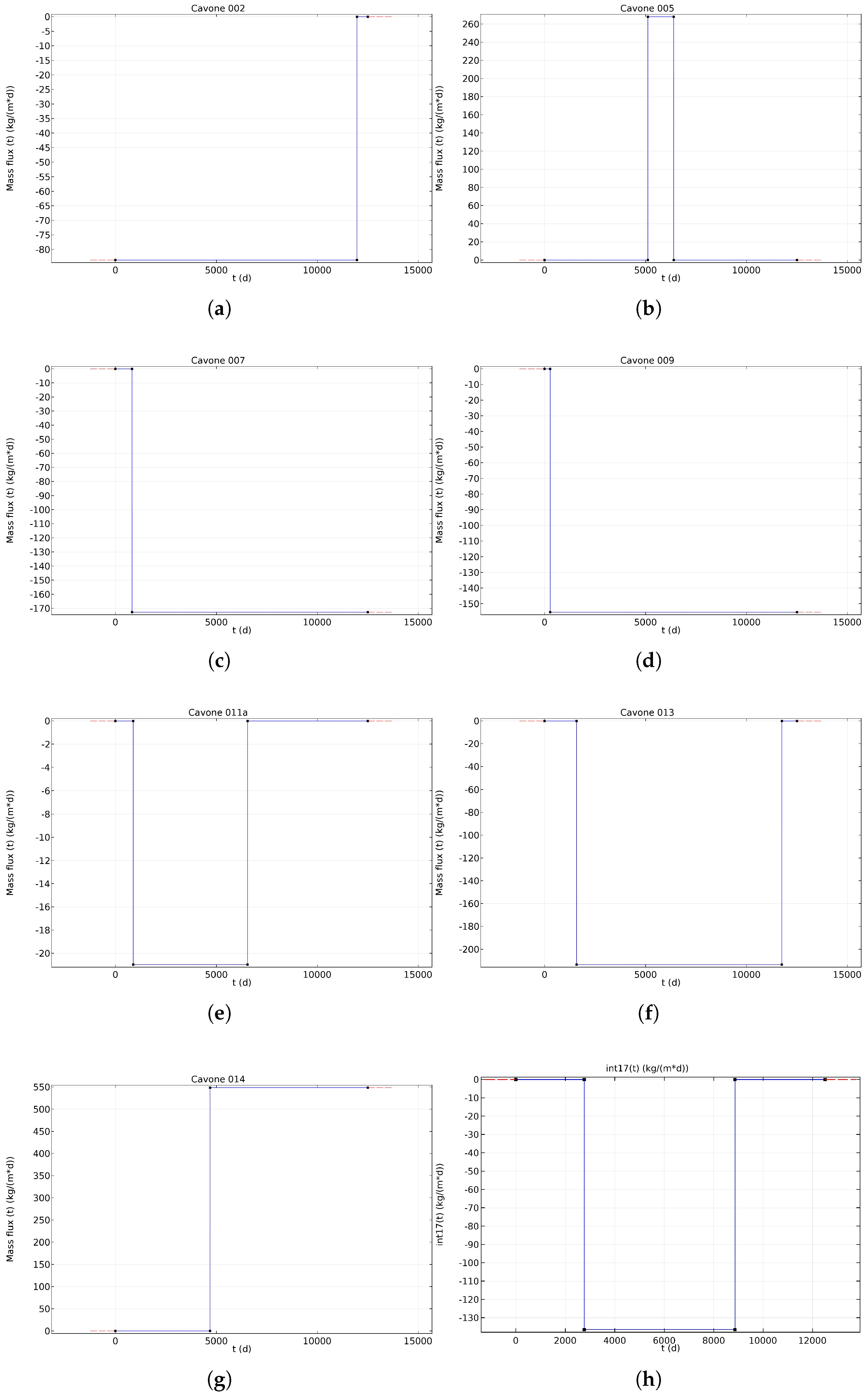
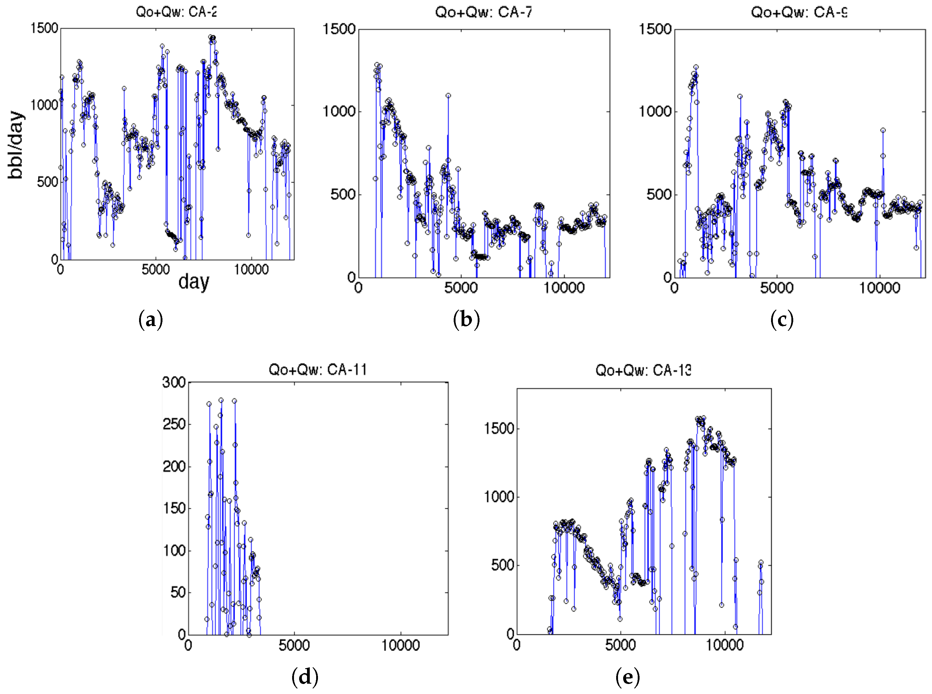
3.2. Production Activity

Wells have been located at the World-Geodetic-System-1984 coordinates furnished by Assomineraria [28]. To this purpose, injection and production volume data have been gathered, and transformed into mass fluxes’ values suited to modeling the wells as lines.

In the Cavone report [7], the injection and production zones were simulated as point sources in a half-space overlain by an impermeable layer. However, the point sources’ depth and the thickness of the impermeable layer were not given. In a first attempt, wells were introduced in COMSOL Multiphysics as small 3D cylinders in a large layered subsurface domain subjected to suitable boundary conditions. This was not very efficient as it required meshing wells with a radius of 0.2 m, namely very small with respect to the surrounding domain. Therefore, each well has been replaced by a source line along its axis [23]. To this purpose, the “well boundary-condition” option offered by COMSOL Multiphysics 5.3 has been exploited. It is based on the Thiem’s solution [29] for homogeneous media written for vanishing well radius and subsequent extension to heterogeneous aquifers through definition of an equivalent conductivity [23]. With the well boundary condition, cylinders are replaced by edges, thus reducing the computational burden associated with fine meshing. This feature was shown to provide accurate solutions compared to modelling the wells as three-dimensional cylinders. Additional data such as the wells’ depth have been deduced from the ICHESE report [30]: the unknown depth values have been assumed equal to an hypothetical but realistic value of 3 km.

An average flux rate has been implemented for each well. All the injection–production rates have been entered in the model as the time-dependent average flux rates shown in Figure 4; mass fluxes produced and injected have negative and positive signs, respectively.

A time dependent simulation has been run over a time interval of 12,510 days, from March 1980 to June 2014.

3.3. Results

According to the available data [7], values of the reservoir permeability $k_{res}$ ranging from 0.3 mD to 1 mD were used. Major pressure change were however associated with smaller values of $k_{res}$. Thus, we choose to show in the current section the results obtained for the lowest data-based value of $k_{res}=0.3$ mD.

The results of the poroelastic analysis are shown for both supported and unsupported reservoir models. More specifically, Figure 5 displays the pressure on the top surface of the reservoir, the shaded surface in Figure 6. In both cases, the major pressure’s increase has been detected near well C014, the main injector of the field, while the pressure’s decreases have been measured near wells C007, C009, and C017. The prominent influence on pressure changes induced by the production activity of well C014 was also fully recognized and investigated by Albano et al. [9]. Though we represent wells as production–injection lines and not as point sources, the obtained pressure values fit with those of the Cavone report [7].

Figure 7 displays the vertical-displacement pattern obtained for both the two-layer and the three-layer models. In fact, the simulated injection–production activities induce subsidence, highlighted by the cold colormap, especially nearby the oilfield, while, expectedly, the entity of the subsidence–induce vertical displacements is sensitive to the layers’ mechanical properties.

4. Modeling the Mirandola Fault and the Cavone Oilfield

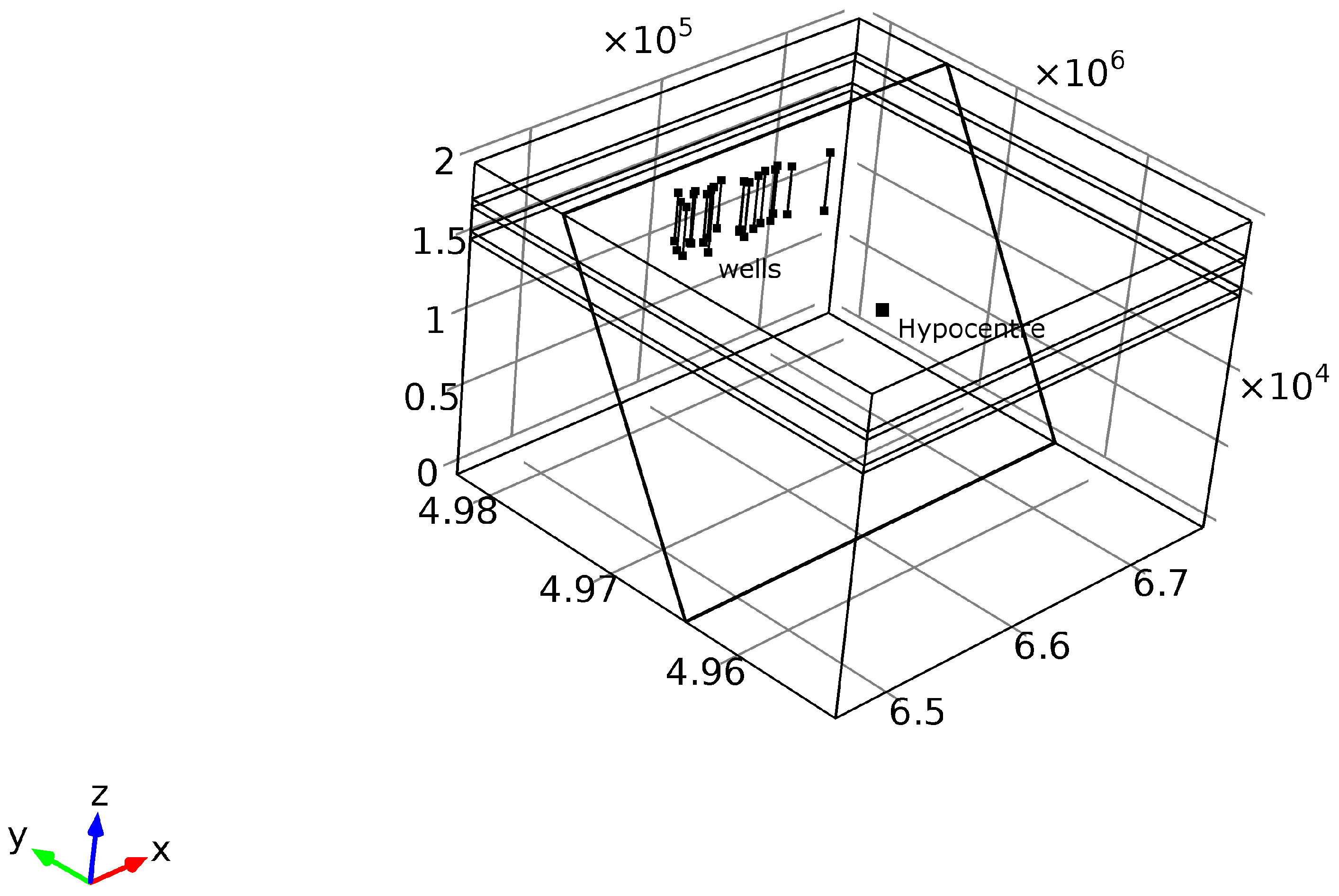
The poroelastic response of a multi-layer block including both the Mirandola fault and the Cavone oilfield has been simulated. Two different subcases have been considered: with and without in situ stresses.

4.1. Model Geometry

A three-dimensional block domain whose dimensions are 30 km × 30 km × 20 km has been modelled, and the model properties of Table 1 have been assigned. The FE model consists of the three-dimensional block in Figure 8 subdivided into five different layers: the upper, the upper caprock, the reservoir, the lower caprock, and, finally, the lower layer.

Different permeability values for each of the layers displayed in Figure 8b have been adopted. The upper caprock layer has very low permeability to avoid communication of the reservoir with the layers above [7], while a lower permeability ranging from 0.1 to 0.001 mD has been assigned to the bottom caprock layer. The reservoir permeability has been set equal to 1 mD for the sake of establishing a comparison with the coupled geomechanical analysis [7], where this value was used.

In the Cavone reservoir, the fault is a sealing stratum for the reservoir. Therefore, the permeability value of the fault is comparatively low, equal to 1 × 10${}^{-9}$ mD. This approach is conservative, as low fault permeability favors slip [31].

Considering that typically the friction coefficient ${\mu }_s$ varies in the interval 0.6–0.85, and that the choice of low ${\mu }_s$ values is conservative [31], ${\mu }_s$ has been assumed equal to 0.6 [32]. Because no information about Skempton’s and Biot’s coefficients were available, the values of 1 and 0.8, respectively, were set [9].

The Mirandola fault has a curved shape, concave to the South, as shown in Figure 1, where the coordinate system is such that the x-axis is easting, the y-axis is northing, and the z-axis is elevation in meters. However, the Mirandola fault has been implemented as a plane to simplify the analysis. When faults are modelled as finite thickness layers with mechanical properties softer than those of the surrounding domain, after imposition of the reverse fault regime by application of in situ stresses, spurious high stress peaks arise near the fault zone and propagate to other parts of the domain. Hence, it has been decided to model the fault zone as a comparatively thin layer of thickness 100 m with the same mechanical properties of the surroundings except for the permeability.

Though blind, the fault has been first modelled as emergent according to the Cavone report [7]. Eventually, it has been modelled as blind to see how results changed.

4.2. Production Activities

We drive the dynamic simulation with well rates as described above.

A production-rate history more accurate than that of Section 3 has been implemented for the major producers and all three injectors according to the Cavone report [7]. The production-rate histories of the other wells are not available from the literature. In particular, the rates history of five producer wells and three injector wells out of nineteen wells are illustrated in Figure 9 and Figure 10, respectively. For the other wells, we exploit the same rate history used in Section 3.

The time interval chosen for the poroelastic simulation covers 11,994 days, from the 1 March 1980 to 31 December 2012. For the time dependent study, a time step of 250 days was used, which is quite small compared to the 11,994 days, to account for the rate fluctuation shown in Figure 9 and Figure 10.

4.3. Mirandola Fault and Cavone Oilfield without In Situ Stress

In a first stage, the changes in effective normal stress, Coulomb Failure Function and pressure have been evaluated in the presence of the oilfield activities without considering the in situ stress state; this extends the case treated in Section 3 by adding the Mirandola fault. These results were obtained on setting the permeability of the lower caprock layer equal to 0.1 mD.

Figure 11 illustrates the color-maps of the changes of shear (a), normal (b) and Coulomb (c) stresses. A very similar colormap, hereby reproduced in Figure 12, was obtained in the Cavone report [7] assuming the reservoir in communication with the underlying aquifer. It is worth noting that the region of influence extends above and below the reservoir: the reservoir expansion due to injection near well C014 increases the effective normal compression above and below the reservoir, in blue on the contour map. Where production is the main activity, the consequent reservoir contraction leads to a drop in the effective compressive normal traction, highlighted in red in the colourmap. In Figure 11c, in the production areas, redthe Coulomb Failure Function change dCFF (2) is positive below the reservoir and negative above it, while colours invert in the injection areas, especially near the C014 well. As suggested in the Cavone report [7], contraction leads to up-dip and down-dip shear traction on the layers below and above the reservoir, respectively. However, the C014 injector induces expansion of the reservoir, and, thus, in its surroundings, the changes are opposite. Furthermore, reservoir contraction leads to a drop in the effective compressive normal traction (red color) in the reservoir depth interval as well as below the reservoir, except near C014 where injection-induced expansion causes an increase in the effective normal compression above and below the reservoir (blue in Figure).

However, at the hypocentre of the May 29th earthquake, whose location (1,664,840 m, 4,968,610 m, −10,200 m) is displayed in Figure 13, the present simulation does not furnish values of dCFF comparable with those of the Cavone report. Hence, a more refined analysis accounting for the in situ stress state has been performed, as discussed in Section 5.

5. Coulomb Stress Changes

For each value of permeability of the lower caprock layer, two different models were set up. The former, called model (0), can be regarded as an “initial” condition; it takes into account the in situ stress and neglects the oilfield activities. The latter model, coined model (1), takes into account both in situ stress and wells activities. Assuming that application of the effects superposition is allowed, the changes of normal, shear and Coulomb stresses have been computed by subtracting the stress values obtained for model (0) from those established in model (1).

5.1. In Situ Stress Field

In situ stresses are prescribed to be lithostatic in the vertical direction, twice the lithostatic in north–south, and 1.5 times the lithostatic in the east–west direction. The lithostatic gradient is calculated with the bulk density assumed to be 2600 kg/m${}^3$. Rollers were applied to each external surface of the three-dimensional domain except the top surface, which is traction-free, and the northern face, on which an external load equal to the in situ stress in the y-direction was applied [7]. All boundaries are no-flow boundaries. Figure 14 displays the adopted boundary conditions.

Let ${\sigma }_1$, ${\sigma }_2$ and ${\sigma }_3$ denote the principal stresses in order of descending magnitude. The typical in situ stress field of Mirandola fault region for z starting from the bottom is [7]

$$\begin{array}{c}{\sigma }_1={\sigma }_{yy}={\sigma }_H=2\rho g(z-h),\hfill \\ {\sigma }_2={\sigma }_{xx}={\sigma }_h=1.5\rho g(z-h),\hfill \\ {\sigma }_3={\sigma }_{zz}={\sigma }_v=\rho g(z-h),\hfill \end{array}$$

(11)

where, according to the Andersonian notation for reverse fault conditions of Figure 15, ${\sigma }_v$ is the vertical stress, while ${\sigma }_H$ and ${\sigma }_h$ are the maximum and minimum horizontal stresses, respectively. We have verified on different FE software besides Comsol that, to get corrected results, the in situ horizontal stresses have to be imposed as internal stresses, and the in situ vertical stress should not be prescribed as internal stresses but through the specific gravity tool of the adopted software.

5.2. Variable Lower Caprock Permeability

The results are plotted at points located within the hanging-wall block, where all the Cavone wells are placed. Stresses have been plotted close to, but not exactly at, the hypocentre, namely 1 km in the negative y-direction from the hypocentre, in order to avoid incurring stress oscillations on the fault.

Figure 16 illustrates the changes in Coulomb failure function $dCFF$ (a) and effective stress $d{\sigma }_n^{\prime }$ (b), respectively. It is noteworthy that, as the pore pressure increases, the Coulomb Failure Function and the effective normal stress increase. The results are plotted for values of permeability of the lower caprock layer ranging from 0.1 mD to 0.001 mD. Remarkably, the displayed pressure changes are displayed following the Cavone report sign convention. In particular, as the permeability of the lower caprock decreases, the pore pressure increases. Simultaneously, the Coulomb Failure Function CFF increases, favoring fault reactivation. Interestingly, the maximum dCFF attained at the end of the simulation, namely when the 2012 earthquakes occurred, is around 0.03 bar.

The trends computed in the Cavone report are plotted with black thick lines. The obtained profiles do not exactly superpose with those reported in the Cavone report. However, the computed values are in the same range of magnitude as that of reference. For a value of permeability of the lower caprock layer equal to 0.1 mD, corresponding to the profiles indicated with the dashed lines, at the time at which the 2012 earthquakes occurred, the positive part of the $dCFF$ in Figure 16a, namely the dCFF that can trigger earthquakes, are quantitatively similar to those of the Cavone report [7].

5.3. Results at Different Distances from the Hypocentre

The spatial variability of the stresses has been checked. In particular, at the locations indicated in Figure 17 having different distances from the hypocentre, the results have been plotted along the negative y-axis in Figure 18, and keeping a constant value of $k_{lower}$ equal to 0.1 mD. It can be drawn that the Coulomb stress change $dCFF$ decreases for increasing distances from the fault on the hanging-wall block.

To check how results change if we move towards the oilfield, the locations indicated in Figure 19 have been selected, where points from A to E gradually move from the hypocentre westward and then towards the Cavone well C014. The corresponding results have been plotted in Figure 20.

As can be inferred from Figure 20a, the Coulomb stress change dCFF below the reservoir decreases when approaching well C014. This conclusion is consistent with those established in the Cavone report [7] and displayed in Figure 12. Once again, the positive values of dCCF, namely those that are assumed to induce seismogenic effects, are consistent with those reported in the Cavone report. On the other hand, the computed negative peaks of dCFF are smaller and are delayed with respect to those of the Cavone report, the difference decreasing when approaching the wells. The negative peaks occur at the peak of the injector well C014, as it can be drawn from Figure 10b. Hence, the present model is particularly sensitive to the activity injection of well C014. Note that, here, the wells have been modelled as line sources and not as point sources as in the Cavone report [7].

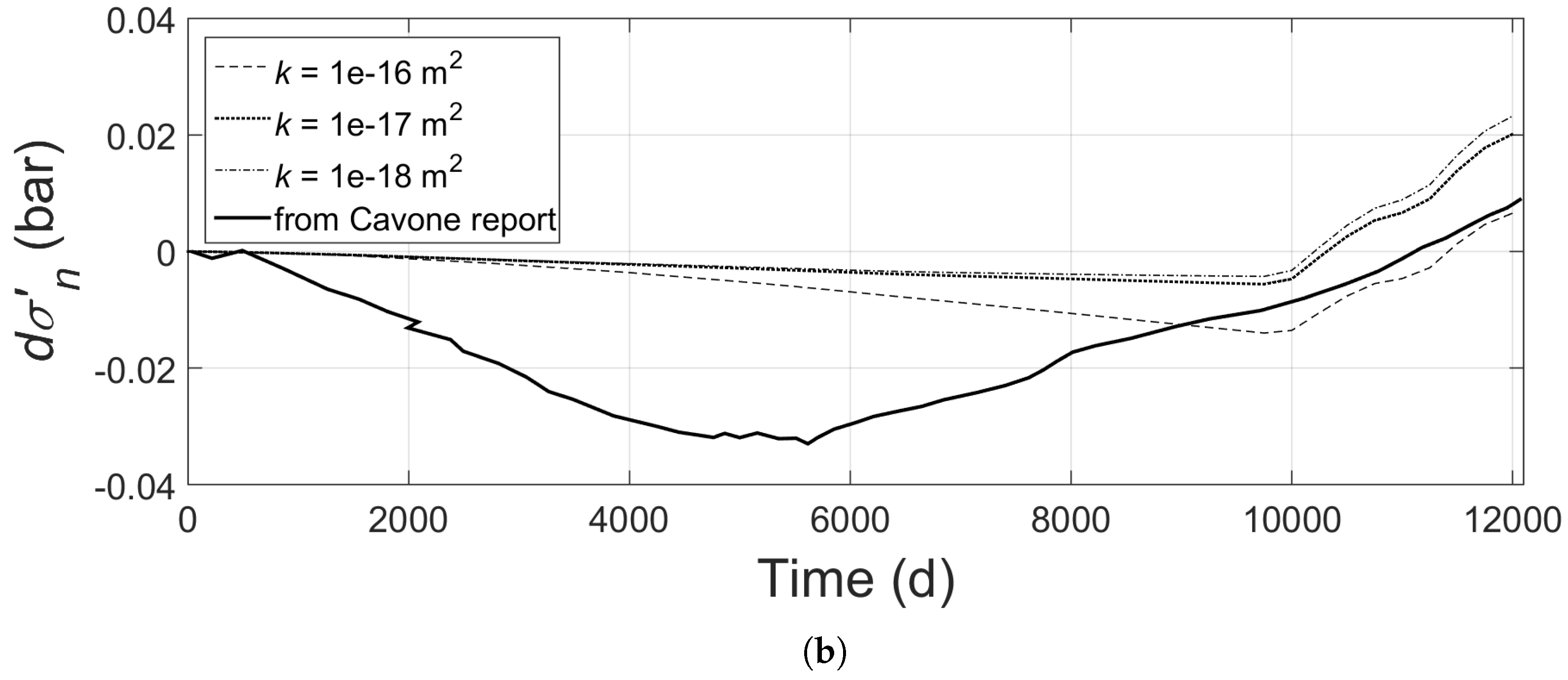
5.4. Blind Fault: Results at the Hypocentre for Variable Lower-Caprock’s Permeability

As shown in Figure 1, according to Cavone seismic profiles, the Mirandola fault does not reach the Earth surface. The authors of the Cavone report [7] considered the fault cutting the entire domain only to facilitate the geometry-mesh building. During the simulation, the upper part of the fault was locked in order to avoid effects on the results. In the present study, to get a more realistic fault representation, the additional model of the blind fault of Figure 21 has been implemented. The material properties of the model and the boundary conditions are the same as in the case with the emergent fault.

The same parametric analysis of the emergent fault case has been repeated. Remarkably, the results of Figure 22 are quite similar to those of the previous cases of non-emergent fault, except that the maximum dCFF slightly decreases, from 0.03 bar to 0.025 bar, suggesting that the fault emergence might not significantly affect the seismicity induced by the Cavone oilfield.

6. Discussion

The minimum stress change that is often recognised to potentially trigger seismicity by static stress transfer is around 0.1 bar [33]. For the Emilia seismic sequence, Pezzo et al. [34] computed a Coulomb stress change induced by the May 20th earthquake on the May 29th fault plane of about 6 bar, and suggested that the May 29th aftershock can be considered as the result of static stress changes from the earlier event.

The present results have shown that the positive change in Coulomb stress near the hypocentre of May 29th as a result of injection activities is very small compared to the Coulomb stress changes calculated at the May 29th hypocentre from the May 20th mainshock. In particular, the positive Coulomb stress change presently computed does not exceed a value of 0.03 bar, against the 0.02 bar established by the authors of the Cavone report [7], anyway, a value largely smaller than 6 bar.

It is commonly expected that earthquakes triggered by fluid injection occur in a radius of few kilometers around the injection well with the highest pressure. The obtained results suggest that fluid injection in the Cavone well C014 may have not caused earthquakes migration, even if injection activities have affected the Cavone field for more than 20 years. Fluid injection at well C014 generated a significant positive Coulomb stress change [9]. However, this change is almost localised in the vicinity of the well C014, namely sufficiently far from the May 29th hypocentre location. The same conclusion was also drawn by Albano et al. [9].

The present simulations have highlighted the role played by the choice of the permeability of the lower caprock layer on the determination of the maximum dCFF reached at the May 29th hypocenter. Remarkably, this conclusion is linked to the idea illustrated in the Cavone report that assuming or not the reservoir as supported by the bottom aquifer is key to a realistic evaluation of the stress field.

The possible emergence of the fault has been shown to slightly smooth the dCFF increments at the hypocenter.

The present study does not answer the question of whether pressure changes may have indirectly altered the time of occurrence of the 29 May 2012 event. Assuming that the main shocks of May 2012 had a tectonic origin, and the May 20th earthquake triggered the May 29th by Coulomb stress transfer, it should be established whether anthropogenic activity and its consequent perturbation of the stress or fluid pressure might have advanced the time of the second seismic event near the Cavone oilfield.

Finally, the FE poroelastic simulation can certainly be further improved, for instance, by simulating the real thrust fold conformation, and modelling the fluid in the reservoir as a multi-phase fluid [35], following, for instance Jha’s high-resolution numerical scheme for the stable simulation of the viscous fingering process [20] and mixing process in viscously unstable laminar flows. However, it should be said that these limitations have not jeopardised the possibility of computing reliable values of potentially seismogenic Coulomb stress changes.

7. Conclusions

Proceeding through subsequent, increasingly complex problems, the present study has illustrated a simplified, coupled fluid-flow-poroelastic analysis for evaluating the seismogenic potential of oil extraction activities in the present case-study. The main finding is that the Coulomb stress change associated with Cavone oilfield activities is two orders of magnitude smaller than that computed on the Mirandola fault in the area where the May 29th event nucleated for the May 20th earthquake. Hence, the present analysis suggests that the seismic events of May 2012 seem not to have been directly triggered by the activity at the Cavone oilfield.

References

1. McGarr, A. Maximum magnitude earthquakes induced by fluid injection. J. Geophys. Res. Solid Earth 2014, 119. [Google Scholar] [CrossRef]
2. Grigoli, F.; Cesca, S.; Rinaldi, A.; Manconi, A.; López-Comino, J.A.; Clinton, J.; Westaway, R.; Cauzzi, C.; Dahm, T.; Wiemer, S. The November 2017 Mw 5.5 Pohang earthquake: A possible case of induced seismicity in South Korea. Science 2018, 360. [Google Scholar] [CrossRef] [PubMed]
3. Dempsey, D.; Suckale, J. Physics-based forecasting of induced seismicity at Groningen gas field, the Netherlands. Geophys. Res. Lett. 2017, 44. [Google Scholar] [CrossRef]
4. Convertito, V.; Catalli, F.; Emolo, A. Combining stress transfer and source directivity: The case of the 2012 Emilia seismic sequence. Sci. Rep. 2013, 3, 3114. [Google Scholar] [CrossRef]
5. King, G.; Stein, R.; Lin, J. Static stress changes and the triggering of earthquakes. Bull. Seismol. Soc. Am. 1994, 84, 935–953. [Google Scholar]
6. Cappa, F.; Rutqvist, J. Modeling of coupled deformation and permeability evolution during fault reactivation induced by deep underground injection of CO2. Int. J. Greenh. Gas Control. 2011, 5, 336–346. [Google Scholar] [CrossRef]
7. Astiz, L.; Dieterich, J.; Frohlich, C.; Hager, B.; Juanes, R.; Shaw, J. On the Potential for Induced Seismicity at the Cavone Oilfield: Analysis of Geological and Geophysical Data, and Geomechanical Modeling. Technical Report. 2014. Available online: http://labcavone.it/documenti/32/allegatrapporto-studiogiacimento.pdf (accessed on 1 July 2014).
8. Juanes, R.; Jha, B.; Hager, B.; Shaw, J.; Plesch, A.; Astiz, L.; Dieterich, J.; Frohlich, C. Were the May 2012 Emilia-Romagna earthquakes induced? A coupled flow-geomechanics modeling assessment. Geophys. Res. Lett. 2016, 43, 6891–6897. [Google Scholar] [CrossRef] [Green Version]
9. Albano, M.; Barba, S.; Tarabusi, G.; Saroli, M.; Stramondo, S. Discriminating between natural and anthropogenic earthquakes: Insights from the Emilia Romagna (Italy) 2012 seismic sequence. Sci. Rep. 2017, 7, 282. [Google Scholar] [CrossRef]
10. Minkoff, S.; Stone, C.; Bryant, S.; Peszynska, M.; Wheeler, M. Coupled fluid flow and geomechanical deformation modeling. J. Pet. Sci. Eng. 2003, 38, 37–56. [Google Scholar] [CrossRef]
11. Dean, R.; Gai, X.; Stone, C.; Minkoff, S. A comparison of techniques for coupling porous flow and geomechanics. Soc. Pet. Eng. J. 2006, 11, 132–140. [Google Scholar] [CrossRef]
12. Rutqvist, J.; Birkholzer, J.; Tsang, C.F. Coupled reservoir–geomechanical analysis of the potential for tensile and shear failure associated with CO2 injection in multilayered reservoir–caprock systems. Int. J. Rock Mech. Min. Sci. 2008, 45, 132–143. [Google Scholar] [CrossRef]
13. Rinaldi, A.P.; Rutqvist, J.; Cappa, F. Geomechanical effects on CO2 leakage through fault zones during large-scale underground injection. Int. J. Greenh. Gas Control. 2014, 20, 117–131. [Google Scholar] [CrossRef]
14. Pruess, K.; Oldenburg, C.; Moridis, G. TOUGH2 User’S Guide Version 2; Lawrence Berkeley National Laboratory: Berkeley, CA, USA, 1999.
15. Itasca. FLAC3D, Fast Lagrangian Analysis of Continua in 3 Dimensions, version 2.0; Itasca Consulting Group, Inc.: Itasca, MS, USA, 2006. [Google Scholar]
16. Cao, H. Development of Techniques for General Purpose Simulators. Ph.D. Thesis, Stanford University, Stanford, CA, USA, 2002. [Google Scholar]
17. Pan, H.; Cao, H. User Manual for General Purpose Research Simulator; Stanford University Petroleum Research Institute: Stanford, CA, USA, 2010. [Google Scholar]
18. Aagaard, B.; Kientz, S.; Knepley, M.; Somala, S.; Strand, L.; Williams, C. PyLith User Manual, version 1.7. 1; Computational Infrastructure for Geodynamics: Davis, CA, USA, 2012. [Google Scholar]
19. Aagaard, B.T.; Knepley, M.G.; Williams, C.A. A domain decomposition approach to implementing fault slip in finite-element models of quasi-static and dynamic crustal deformation. J. Geophys. Res. Solid Earth 2013, 118, 3059–3079. [Google Scholar] [CrossRef] [Green Version]
20. Jha, B. Flow through Porous Media: From Mixing of Fluids to Triggering of Earthquakes. Ph.D. Thesis, Massachusetts Institute of Technology, Cambridge, MA, USA, 2014. [Google Scholar]
21. Jha, B.; Juanes, R. Coupled multiphase flow and poromechanics: A computational model of pore pressure effects on fault slip and earthquake triggering. Water Resour. Res. 2014, 50, 3776–3808. [Google Scholar] [CrossRef] [Green Version]
22. Juanes, R.; Samper, J.; Molinero, J. A general and efficient formulation of fractures and boundary conditions in the finite element method. Int. J. Numer. Methods Eng. 2002, 54, 1751–1774. [Google Scholar] [CrossRef]
23. Indelman, P.; Dagan, G. A note on well boundary condition for flow through heterogeneous formations. Water Resour. Res. 2004, 40, 1–7. [Google Scholar] [CrossRef]
24. Cocco, M.; Rice, J. Pore pressure and poroelasticity effects in Coulomb stress analysis of earthquake interactions. J. Geophys. Res. Solid Earth 2002, 107, 2–17. [Google Scholar] [CrossRef]
25. Biot, M. General theory of three-dimensional consolidation. J. Appl. Phys. 1941, 12, 155–164. [Google Scholar] [CrossRef]
26. Rice, J.; Cleary, M. Some basic stress-diffusion solutions for fluid-saturated elastic porous media with compressible constituents. Rev. Geophys. Space Phys. 1976, 14, 227–241. [Google Scholar] [CrossRef]
27. Detournay, E.; Cheng, A.D. Fundamentals of poroelasticity. In Comprehensive Rock Engineering: Principles, Practice and Projects; Pergamon Press: Oxford, UK, 1993; Volume II, Chapter 5; pp. 113–171. [Google Scholar]
28. Assomineraria. Rapporto ambientale 2015—Attività Oil&Gas; Technical Report; Associazione Mineraria Italiana per l’industria Mineraria e Petrolifera: Roma, Italy, 2015. [Google Scholar]
29. Thiem, G. Hydrologische Methoden; J. M. Gebhardt: Leipzig, Germany, 1906. [Google Scholar]
30. Styles, P.; Gasparini, P.; Huenges, E.; Scandone, P.; Lasocki, S.; Terlizzese, F. Report on the Hydrocarbon Exploration and Seismicity in Emilia Region; Technical Report; International Commission on Hydrocarbon Exploration and Seismicity in the Emilia Region (ICHESE), Regione Emilia Romagna: Bologna, Italy, 2014. [Google Scholar]
31. Fan, Z.; Eichhubl, P.; Gale, J. Geomechanical analysis of fluid injection and seismic fault slip for the Mw4. 8 Timpson, Texas, earthquake sequence. J. Geophys. Res. Solid Earth 2016, 121, 2798–2812. [Google Scholar] [CrossRef]
32. Byerlee, J. Friction of rocks. Pure Appl. Geophys. 1978, 116, 615–626. [Google Scholar] [CrossRef]
33. Hardebeck, J.; Nazareth, J.; Hauksson, E. The static stress change triggering model: Constraints from two southern California aftershock sequences. J. Geophys. Res. Solid Earth 1998, 103, 24427–24437. [Google Scholar] [CrossRef] [Green Version]
34. Pezzo, G.; Boncori, J.; Tolomei, C.; Salvi, S.; Atzori, S.; Antonioli, A.; Trasatti, E.; Novali, F.; Serpelloni, E.; Candela, L.; et al. Coseismic deformation and source modeling of the May 2012 Emilia (Northern Italy) earthquakes. Seismol. Res. Lett. 2013, 84, 645–655. [Google Scholar] [CrossRef]
35. Bader, A.; Fisher, Q.; Harris, S. The importance of incorporating the multi-phase flow properties of fault rocks into production simulation models. Mar. Pet. Geol. 2005, 22, 365–374. [Google Scholar]
Figure 1. Location and geometry of Mirandola fault with 2012 earthquakes location reproduced from the Cavone Report [7]: Geologic section showing location and focal mechanism of the May 29th event.
Geosciences 09 00213 g001
Figure 2. Cavone oilfield modeling—two layer reservoir model: geometry (a) and mesh (b); dimensions are in meters.
Geosciences 09 00213 g002
Figure 3. Cavone oilfield modeling—geometry (a) and mesh (b) of the three layers reservoir model, with dimensions in meters.
Geosciences 09 00213 g003
Figure 4. Cavone oilfield modeling: Average mass fluxes of wells C002 (a); C005 (b); C007 (c); C009 (d); C011a (e); C013 (f); C014 (g); and C017 (h).
Geosciences 09 00213 g004
Figure 5. Cavone oilfield modeling: Pressure (bar) colour pattern computed on the top of the reservoir layer (parallel to xy plane) with wells for the unsupported (a) and the supported (b) reservoir models.
Geosciences 09 00213 g005
Figure 6. Cavone oilfield modeling: Top of reservoir layer where pressure is plotted in the three layers model, dimensions being in meters.
Geosciences 09 00213 g006
Figure 7. Cavone oilfield modeling—Vertical displacement or subsidence of the reservoir model at the end of the simulation for the two-layer (a) and the three-layer (b) models; dimensions are in meters.
Geosciences 09 00213 g007
Figure 8. Mirandola emergent fault and Cavone oilfield modeling: geometry (a) and lateral view (b) of the 3D FE model; dimensions are 10 5 m in x, 10 6 m in y and 10 4 m in z.
Geosciences 09 00213 g008
Figure 9. History of the modelled flow rates for five producers, C002 (a); C007 (b); C009 (c); C011a (d); C013 (e). These figures have been taken from [7].
Geosciences 09 00213 g009
Figure 10. History of the modelled liquid flow rates for three injectors, C005 (I) (a), C011b (I) (c) and C014 (I) (b) out of the 19 wells.These figures have been taken from [7].
Geosciences 09 00213 g010
Figure 11. Mirandola fault and Cavone oilfield modeling without in situ stress: Up-dip traction changes d τ in bar (a), effective normal stress change d σ (bar) (b) and Coulomb Failure Function change d C F F (bar) (c). Results are plotted on a vertical plane parallel to xz plane at the end of simulation, namely after 11,994 days.
Geosciences 09 00213 g011aGeosciences 09 00213 g011b
Figure 12. Mirandola fault and oilfield modeling without in situ stress reproduced from the Cavone report [7]: effective tractions and Coulomb stress function change d C F F on the fault on the 11,994 day for the case with bottom aquifer support. The change in the effective normal traction is positive near producers and negative near injectors because pressure depletion leads to contraction of the reservoir and pressure increase leads to increased compression on the fault. The white cross mark on the d C F F plot denotes the hypocentre location.
Geosciences 09 00213 g012
Figure 13. View of the domain with wells and the May 29th earthquake hypocentre.
Geosciences 09 00213 g013
Figure 14. Boundary conditions: Surfaces highlighted in blue are subjected to: rollers restraints (a), and boundary loads (b); dimensions are in meters (10 5 in x-, 10 6 in y- and 10 4 in z-directions).
Geosciences 09 00213 g014
Figure 15. Andersonian notation for the reverse fault regime.
Geosciences 09 00213 g015
Figure 16. Emergent Mirandola fault and Cavone oilfield modeling: Coulomb stress change d C F F (bar) (a); effective normal stress change d σ n (bar) (b) plotted for variable permeability of the lower caprock layer at a distance of 1 km from the hypocentre in the negative y-axis, on the hanging-wall block.
Geosciences 09 00213 g016aGeosciences 09 00213 g016b
Figure 17. Mirandola fault and Cavone oilfield modeling—location of the three points at different distances from the hypocentre in the negative y-direction; (a) prospective view; (b) lateral view; dimensions are in meters (10 5 in x, 10 6 in y- and 10 4 in z-directions).
Geosciences 09 00213 g017
Figure 18. Emergent Mirandola fault and Cavone oilfield modeling: Coulomb stress change d C F F (bar) (a), and effective normal stress change d σ n (bar) (b) plotted for permeability of the lower caprock layer k l o w e r = 0.1 mD at different distances from the hypocentre in the negative y-direction, on the hanging-wall block (see Figure 17).
Geosciences 09 00213 g018
Figure 19. Mirandola fault and Cavone oilfield modeling—Location of points A, B, C, D and E at different distances from the hypocentre; (a) prospective view; (b) lateral view; dimensions are in meters (10 5 in x, 10 6 in y-= and 10 4 in z- directions).
Geosciences 09 00213 g019
Figure 20. Emergent Mirandola fault and Cavone oilfield modeling: results at different points from the hypocentre for permeability of the lower caprock layer k l o w e r = 0.1 mD; Coulomb stress change d C F F (bar) (a) and effective normal stress change d σ n (bar) (b) are plotted for different distances from the hypocentre, on the hanging-wall block (see Figure 19).
Geosciences 09 00213 g020
Figure 21. Blind Mirandola fault and Cavone oilfield modeling: geometry (a), and lateral view of the 3D model (b); dimensions are 10 5 m in x, 10 6 m in y and 10 4 m in z.
Geosciences 09 00213 g021
Figure 22. Blind Mirandola fault and Cavone oilfield modeling: Coulomb stress change d C F F (bar) (a) and effective normal stress change d σ n (bar) (b) evaluated at the hypocentre for variable permeability of the lower caprock layer k l o w e r (1 mD = 10 15 m 2 ).
Geosciences 09 00213 g022