Edge Detectors as Structural Imaging Tools Using Aeromagnetic Data: A Case Study of Sohag Area, Egypt

Abstract

The present study was designed to give a clear and comprehensive understanding of the structural situation in the Sohag region and surrounding area by applying several edge detectors to aeromagnetic data. In this research, the International Geomagnetic Reference Field (IGRF) values were removed from the aeromagnetic data and the data obtained were then reduced to the north magnetic pole (RTP). A combination of different edge detectors was applied to determine the boundaries of the magnetic sources. A good correlation was noticed between these techniques, indicating that their integration can contribute to delineating the structural framework of the area. Consequently, a detailed structural map based on the results was constructed. Generally, E-W, N45-60E, and N15-30W directions represent the main tectonic trends in the survey area. The structural map shows the existence of two main basins constituting the most probable places for hydrocarbon accumulation. The results of this study provide structural information that can constitute an invaluable contribution to the gas and oil exploration process in this promising area. They show also that the decision in choosing the location of the drilled boreholes (Balyana-1 and Gerga) was incorrect, as they were drilled in localities within an area of a thin sedimentary cover.

1. Introduction

Edge detectors have been widely used in geophysical exploration, especially in mapping geologic contacts, faults, dykes, and ore bodies. In the last few decades, several methods have been introduced to improve the delineation process of magnetic anomalies and the definition of the shapes of the causative source bodies regardless of their depths. One of the basic correction filters is the reduction to the magnetic pole which was first introduced by [1] to resolve the asymmetrical shape of anomalies by reproducing the magnetic anomalies with vertical magnetization. The most common enhancement methods that have been routinely used in magnetic data are horizontal and vertical derivatives [2]. These derivatives have been used to emphasize the edges of magnetization boundaries [3].

However, the widespread use of the horizontal and vertical derivatives to determine attenuated anomalies at different ranges is often onerous due to the high amplitude variations in magnetic signals that originate from magnetic sources of different geometries located at different depths with different magnetization properties [4]. The magnetic body and its edges produce indistinct features that impede the study of the magnetic signal behavior in the structural models and make the task of interpretation complicated [5]. Consequently, a number of edge detection techniques based on derivatives have been introduced to overcome such problems and to deal with complex magnetic anomalies. These techniques have become fundamental in figuring out the true boundaries of the magnetic source, as they give a comprehensive view of anomalies and delineate the shape of causative sources regardless of their depths, as well as enhance both deep and shallow structures and balance small and large amplitudes of magnetic anomalies by normalizing derivatives of the field data [6]. Among those techniques are: the first-order vertical derivative [7], Euler deconvolution [8], the total horizontal gradient [9], the analytical signal [10], the tilt angle derivative [11], enhanced horizontal derivative [12], total horizontal derivative of the tilt angle [4], Theta map [13], horizontal tilt angle [14], and the enhanced total horizontal gradient of the tilt angle [2].

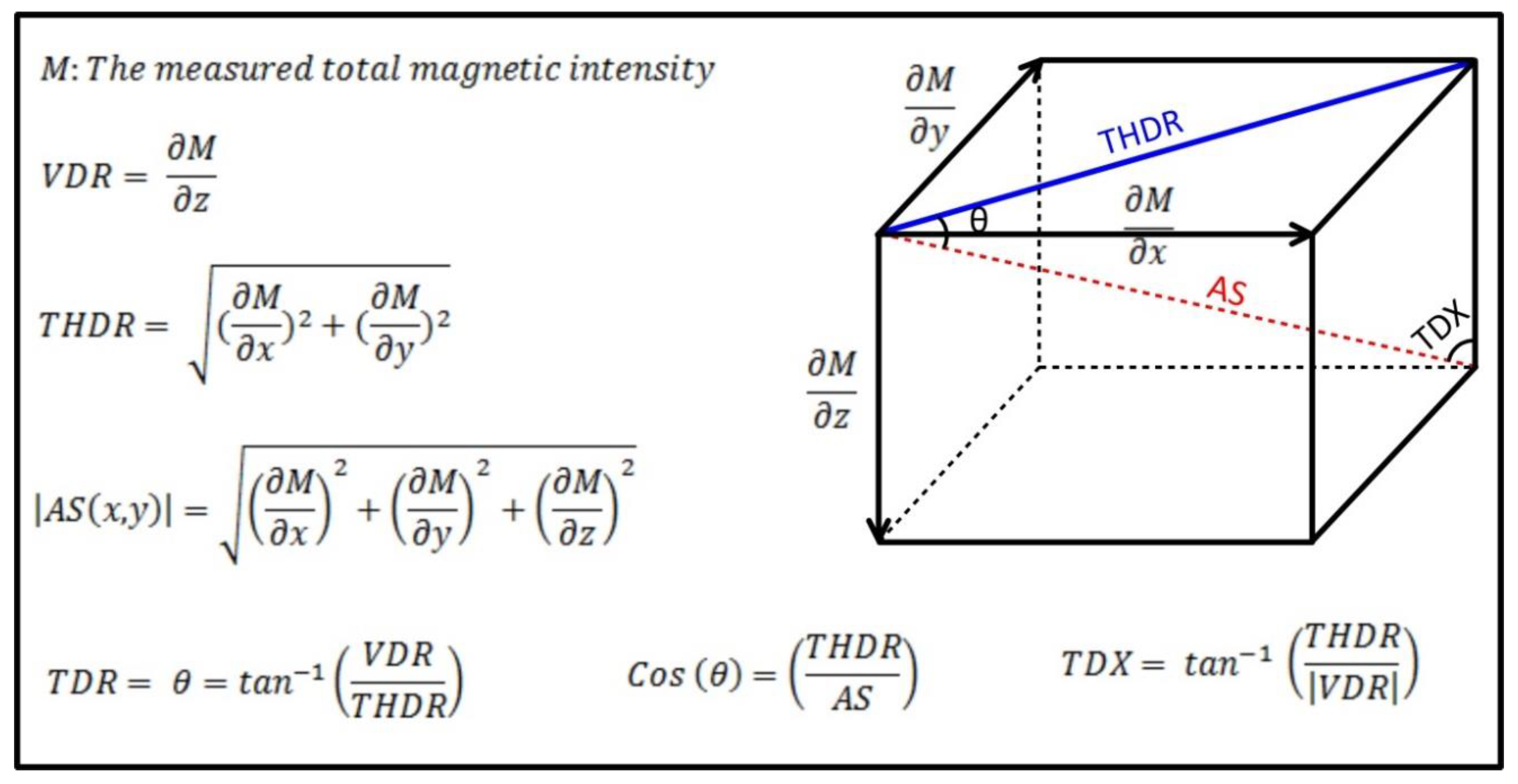
2. Background and Methodology

Many techniques are concerned with the detection of the edges of potential field anomalies generated by geological structures. Nowadays, edge detectors constitute an essential step in the process of potential field data interpretation. The total horizontal derivative (THDR) method has been used extensively to map the boundaries of susceptibility contrasts. It exploits the fact that the horizontal derivative of the RTP magnetic field generated by a tabular body tends to have maximum values over the edges of the anomalous body in case the edges are vertical and well-separated from each other [9]. THDR is not only less sensitive to the noise in the data, but also robust in detection of shallow magnetic sources [15]. It has high amplitude over the edge of the magnetic source and is determined by the following equation [9]:

$$\mathrm{THDR}= \sqrt{(\frac{\partial M}{\partial x}{)}^2+(\frac{\partial M}{\partial y}{)}^2}$$

(1)

where $\frac{\partial M}{\partial x}$ and $\frac{\partial M}{\partial y}$ are the two horizontal derivatives of the observed field ($M$).

The first-order vertical derivative (VDR) was first applied to delineate edges of gravity and magnetic bodies by [7]. It is commonly applied to the data to emphasize near-surface geological features and enhance the high wavenumber components of the spectrum where the zero values of vertical derivatives of the RTP magnetic field commonly correspond to the geological boundaries [16]. It is formulated thus:

$$\mathrm{VDR}=\frac{\partial M}{\partial z}$$

(2)

The analytic signal (AS), which is the square root of the sum of squares of the derivatives in the x, y, and z directions, is applied to determine the magnetic source geometry [10]. The complex analytic signal is specified in terms of the horizontal and vertical derivatives of the total field and the function calculated in the analytic method is the analytic signal amplitude of the potential field [17].

$$\left|\mathrm{AS}\left(x,y\right)\right|=\sqrt{{\left(\frac{\partial M}{\partial x}\right)}^2+{\left(\frac{\partial M}{\partial y}\right)}^2+{\left(\frac{\partial M}{\partial z}\right)}^2}$$

(3)

where, $\left|\mathrm{AS}\left(x‚y\right)\right|$ is the amplitude of the analytic signal at (x, y), $M$ is the observed magnetic field at (x, y), and $\frac{\partial M}{\partial z}$ is the vertical first-order derivatives of the observed field.

The amplitude of the analytic signal reaches its maxima when centered over the source parameter, with bell-shaped anomalies. The shallow sources become dominant if there is more than one source [2]. However, the AS acts poorly in enhancing anomalies generated by the existence of shallow and deep bodies at the same time due to its weakness in balancing the amplitudes of different anomalies [18].

The first normalized edge detection method developed for balancing or equalizing different amplitude edges was the tilt angle (TDR) introduced by [11], but this method still could not clearly determine the boundaries of geologic units as it amplifies noise in the data. The tilt angle function is given by the arctangent of the ratio of the vertical derivative of the potential field to its total horizontal derivative:

$$\mathrm{TDR}= \theta ={\tan }^{-1}\left(\frac{\mathrm{VDR}}{\mathrm{THDR}}\right)$$

(4)

Tilt derivative amplitude variations have a certain range, between −$\pi /2$ and π/2 according to the nature of the arctangent trigonometric function. Its amplitude has three rates: positive over the source, zero at/near the edge of the source, and negative outside the source [19]. In the presence of noise, this technique acts as an effective signal discriminator for both shallow and intermediate sources but becomes blurred for sources at considerable depths, where it can not reveal deep-level geologic boundaries [2]. Although its efficiency reduces with depth, this method produces relatively sharp anomalies and generates better definition of edges over the body [4].

Another balanced method proposed by [13] is the Theta map (Cos ($\theta$)). It uses the AS amplitude to normalize the THDR in a 2D image. Using the Theta map, the amplitude of the response from the sources situated at different depths is similar despite the fact that the response from deeper sources is more diffuse [14]. This technique can detect edges regardless of strike and amplitude [16]. It is calculated using the following equation:

$$\mathrm{Cos} \left(\theta \right)=\left(\frac{\mathrm{THDR}}{\mathrm{AS}}\right)$$

(5)

where 0 < θ < π/2 as it relies on the horizontal gradient, which is always positive.

The horizontal tilt angle (TDX) [14] is the amplitude of the horizontal gradient that is normalized to the absolute value of the vertical derivative. It can be represented as follows:

$$\mathrm{TDX}= {\tan }^{-1} \left(\frac{\mathrm{THDR}}{\left|\mathrm{VDR}\right|}\right)$$

(6)

TDR works effectively with data from shallow sources, but it is considered relatively ineffective when dealing with data from deep sources. TDX is the inverse of the TDR proposed, as it performs equally well with both shallow and deep sources. One disadvantage of this method is that it reflects edges greater than the actual body size in the case that more than one causative body with various geometries exists [14]. The geometric relationship between VDR, THDR, AS, $Cos \left(\theta \right)$, TDR, and TDX are shown in Figure 1.

As the horizontal gradient method has the ability to determine both shallow and deep structures [15] and a low sensibility to noise [14], Arisoy et al. [2] developed a new technique using the horizontal gradient, based on the ETilt filter, in order to overcome the domination of high amplitude that makes anomalies resulting from THDR and AS methods insensitive to a wide range of amplitudes. This technique is the enhanced total horizontal gradient of tilt angle (ETHDR) method.

$$\mathrm{ETilt}={\tan }^{-1}(\frac{K\left(\frac{\partial M}{\partial z}\right)}{\sqrt{{\left(\frac{\partial AS}{\partial X}\right)}^2+{\left(\frac{\partial AS}{\partial y}\right)}^2}})$$

(7)

$$\mathrm{ETHDR}=\sqrt{{\left(\frac{\partial \mathrm{ETilt}}{\partial X}\right)}^2+{\left(\frac{\partial \mathrm{ETilt}}{\partial y}\right)}^2}$$

(8)

where $K=\frac{1}{\sqrt{\Delta x^2+\Delta y^2}}$ is the dimensional correction factor, and ∆x and ∆y are the sampling intervals in the x and y directions, respectively.

This technique emphasizes subtle magnetic anomalies as it has the same behavior as the vertical derivative, with zero contour indicating the edge or source. This filter is more powerful than others in delineating the edges of both shallow and deep bodies, even with the existence of several magnetic sources. Unfortunately, the ETilt and ETHDR methods use second derivatives, so they are not able to discriminate between edges and noise in case of relatively high levels of noise [2].

Euler deconvolution (ED) was introduced by [8] as an automatic interpretation technique for estimating the location of 2D magnetic causative sources along profile data. Later, [20] applied the technique to gridded data. It has become one of the most widely used semi-automatic interpretation tools for potential field data due to its simplicity of implementation, as well as that the fact it performs automatic estimation of anomalous source locations and their depths [21]. It also has the advantage that its results are not influenced by the existence of remnant magnetization [22]. The method can be applied to huge data sets using the moving window technique, where the structural index (SI) must be assumed before applying the technique. This is a critical procedure as the estimated depth can be greatly affected by using the wrong structure index [23,24]. Like all the techniques introduced above, noise may be increased in the data as the Euler technique uses first-order derivatives. The window size must also be chosen carefully to enhance features from the depths of interest and exclude unreliable solutions [23]. The 3D ED requires two horizontal and vertical gradients of the potential field, calculated using the fast Fourier transform. Euler’s homogeneity equation in grid (3D) form can be written as follows [8,20]:

$$N\left(B-M\right)=\left(x-x_0\right)\frac{\partial M}{\partial x}+\left(y-y_0\right)\frac{\partial M}{\partial y}+\left(z-z_0\right)\frac{\partial M}{\partial z}$$

(9)

where M is the observed field at the locations (x, y, z), (x₀, y₀ and z₀) are the coordinates of the source location, B is the base level of the field, and N is the structural index which is a function of the source geometry of the causative bodies.

3. Application to the Aeromagnetic Data of the Sohag Area, Egypt

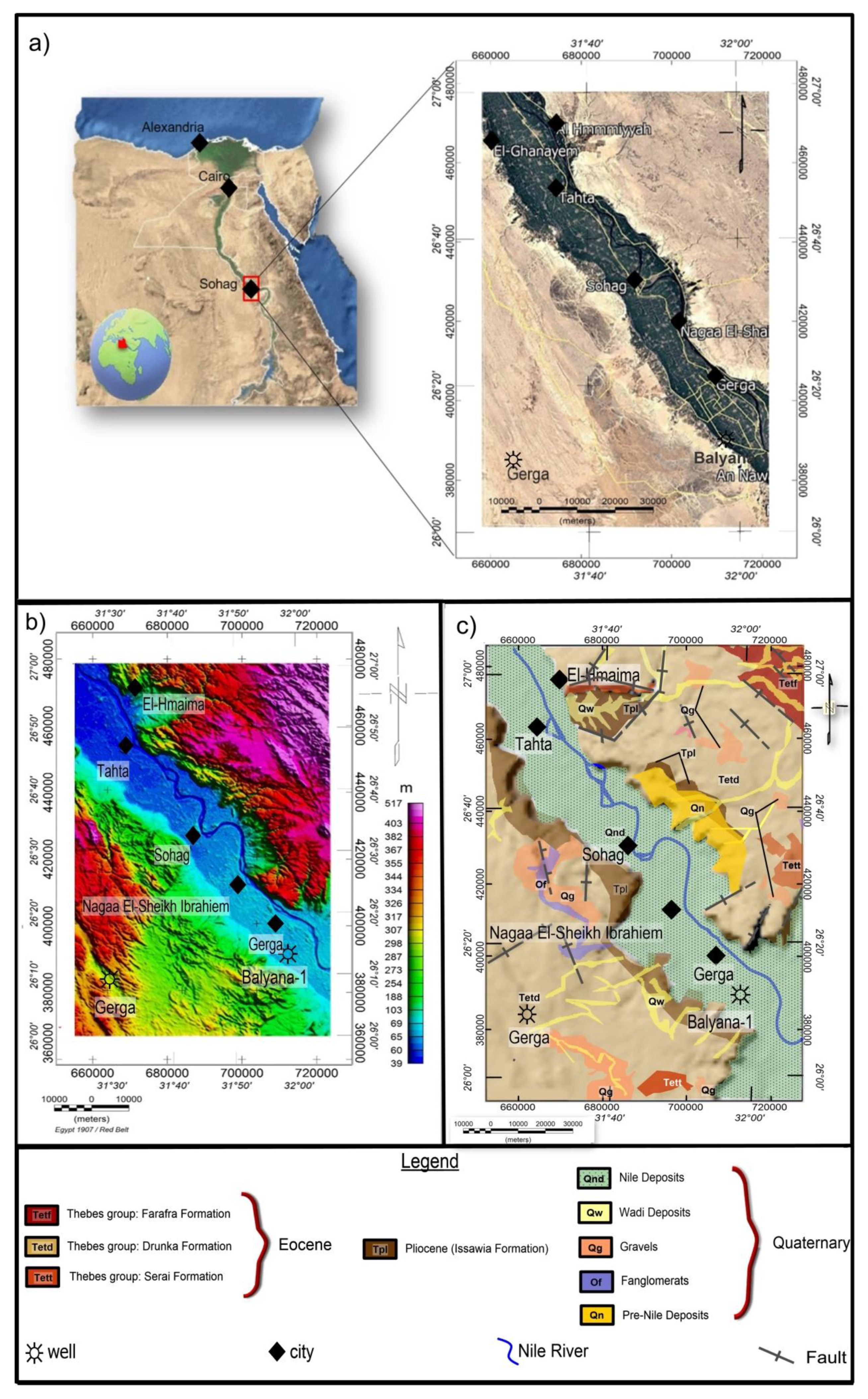
3.1. Location, Geology, and Structure of the Study Area

The area of study is situated in the southern Nile Valley region of Egypt and extends between longitudes 31°30′ and 32°00′ E, and latitudes 26°00′ and 27°00′ N (Figure 2a). Despite it lying mostly within the stable shelf belt, the study area is considered an ambiguous area with complex structural settings due to the acute shortage of surface and subsurface structural information [25] and the lack of exploratory wells and previous geophysical studies. The Balyana-1 exploratory well is the only borehole in the study area that reaches to the basement at a depth of 1640 m, while the Gerga well reaches a depth of 492 m within the Eocene formation (Figure 2). The report of the Balyana-1 well provides information about the presence of uneconomic gas accumulations within the interval between the clay-stone and the siltstone of the Quaternary sediments of the Nile Valley fill. The shale and the coal of the Cretaceous can also contribute to the petroleum system in the area in case of the availability of appropriate conditions of pressure and temperature to generate hydrocarbons. This information leads to the necessity to reassess the structural settings of the area and determine the most suitable places for drilling new boreholes.

The Nile Valley, which is bounded by the eastern and western Eocene limestone plateaus, lies nearly horizontal, and rocks in the valley have a gentle north-northwest (NNW) regional dip [26]. The eastern plateau is more highly dissected by normal faulting than the western plateau with an elevation ranging between 350 and 500 m above mean sea level, compared to 250 to 350 m on the western plateau [27] (Figure 2b). The geologic map of the study area (Figure 2c) shows that the surface geology is from the Eocene to Quaternary age.

The Nile Valley region can be described geologically, according to [25,29], from older to younger units as: The Thebes group (Serai and Drunka formations of Lower Eocene), first introduced by [30] and mainly consisting of limestone [31]. It has an average thickness of about 200 m with highly fossiliferous content composed of thick-bedded limestone and chert bands with marl at the base. Overlaying the Thebes Formation, the Issawia Formation (Pliocene) consists of about 70 m of brown marls and clay, limestone, and conglomerate. The flood plain (cultivated lands) on top of the Issawia Formation is composed mainly of alluvium sediments restricted along the narrow tract of the Nile Valley. Quaternary deposits are represented by the pre-Nile deposits, alluvial fanglomerates, Wadi deposits, and Playa deposits. To the southeast of Gerga city, Precambrian basement rock fragments were found within Qena and Abassia Formations [25]. The subsurface stratigraphy was inferred from the lithology of the Balyana-1 well [24], where it encounters the Precambrian crystalline basement at a depth of 1640 m. The subsurface sediments belong to the Cretaceous, Tertiary, and Quaternary [32]. It is worth to mention that an uneconomic amount of gas was reported at a depth of 880 m within the Nile Valley fill sediments. The following

Table 1. Lithology of the Balyana-1 well.

Age	Epoch	Formation	Lithology	Depth (m)
Quaternary	Holocene	Nile Valley fill	Pebbly sandstone, siltstone, and shales being fossiliferous with coal fragments.	893.7
Tertiary	L. Eocene	Esna	Calcareous shale with sandstone, siltstone, and marl.	1264.9
Cretaceous	Campanian	Duwi	Chalk, silt, and sandstone.	1330.2
	Coniacian	Quseir	Siltstone with coal and sandstone consolidated with clay-stone.	1520.7
		Taref	Claystone and kaolinitic sandstone with shale and feldspar.	1640.4
Pre-Cambrian		Granitic wash		1656.3
		Basement		1737.1

shows the lithology of the Balyana-1 borehole.

The structural trends affecting the stable shelf of Egypt are classified by [25] into four categories: E-W, NE-SW, N-S, and NW-SE. Studies conducted by [33,34] using satellite imagery referred to the existence of a large number of structurally controlled superficial fractures oriented in the NW-SE direction with dextral (right lateral) movements in relatively recent times (Plio-Pleistocene). The combination of the NW-SE fractures has been explained as conjugated sets due to the compression stress produced in the north-northeast (NNE) direction [35]. The presence of some intrusive bodies of granodiorite rock type in the area of study has been identified [36].

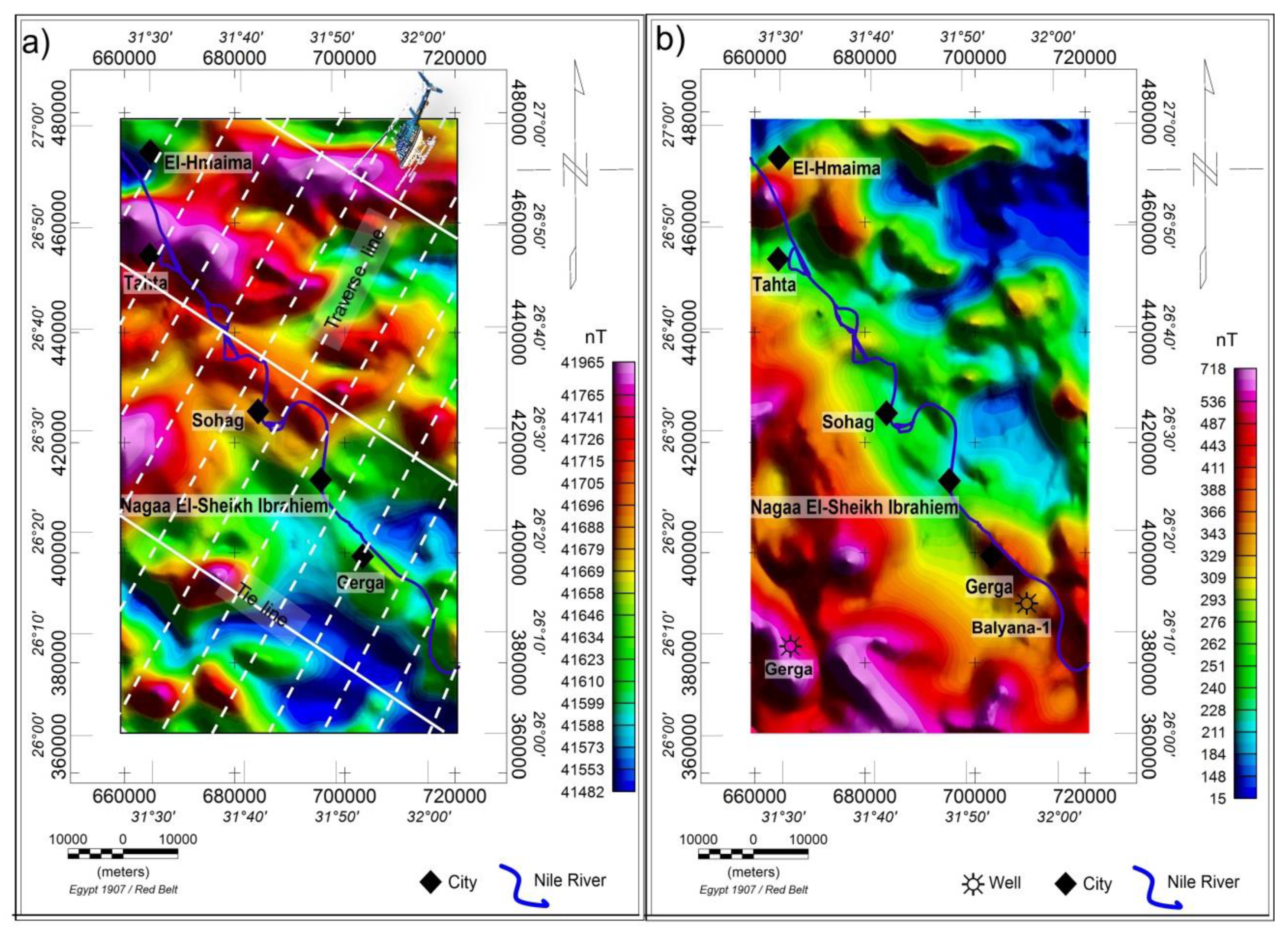
3.2. Airborne Geophysical Magnetic Data

The magnetic survey was acquired by the Aero Service Division of the Western Geophysical Company of America [37] using the airborne Varian V-85 proton free-precession magnetometer with a sensitivity of 0.1 nT along parallel flight lines oriented in a NE-SW direction and an azimuth of 45°/225° at 1.5 km spacings. Tie lines were flown in a NW-SE direction normal to the main flight line direction with approximately 5 km intervals. The flight altitude was 914.4 m. The inclination and the declination of the magnetic field were 39.5° N and 2° E, respectively.

The data has been digitized from three sheets with a scale of 1/50,000 and contour intervals of 10 nT, then gridded using the minimum curvature method with a grid cell of 500 m to form the total magnetic intensity map of the investigated area (Figure 3a). The International Geomagnetic Reference Field (IGRF) values were subtracted to remove the regional effects of the earth’s magnetic field. The data obtained was reduced to the north magnetic pole—assuming only induced magnetization—using fast Fourier transform (FFT) to overcome undesired distortion in the shapes, sizes, and locations of magnetic anomalies, due the effect of the inclination and declination of the magnetic field. Thus, the RTP transformation provides a more accurate estimate of the positions of magnetic sources and the shape is easier to interpret in terms of the body. The RTP magnetic map (Figure 3b) shows that the area is separated into two main belts; a low magnetic anomaly belt (could be associated with deep basement rocks overlaid by thick low-magnetized sediments) lies at the northeastern part of the area, and a high magnetic belt located at the southwestern and northwestern parts reflects a shallow depth of magnetic sources (uplifted basement blocks and/or igneous intrusions). The Nile Valley extends approximately along the border between these belts. Magnetic values range from 15 to 718 nT.

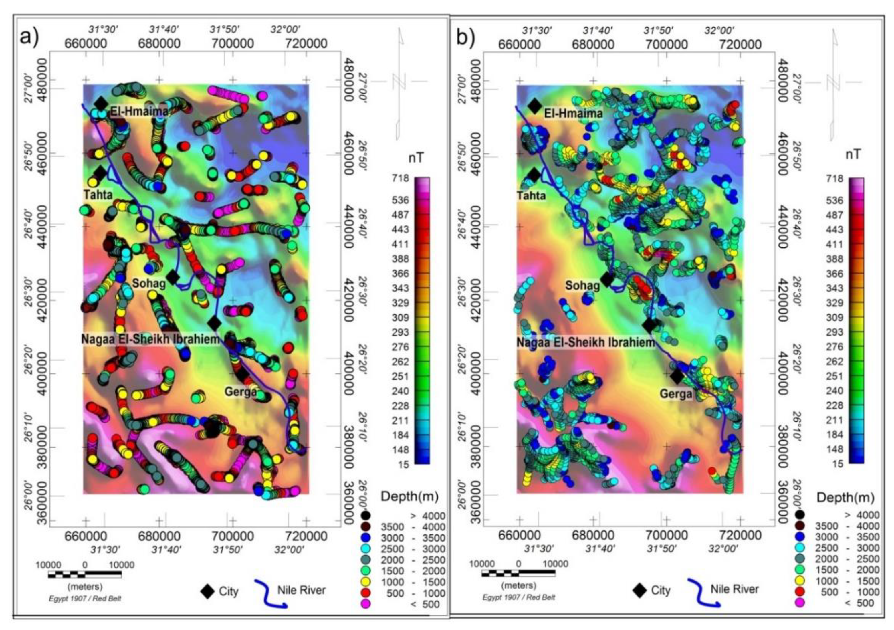
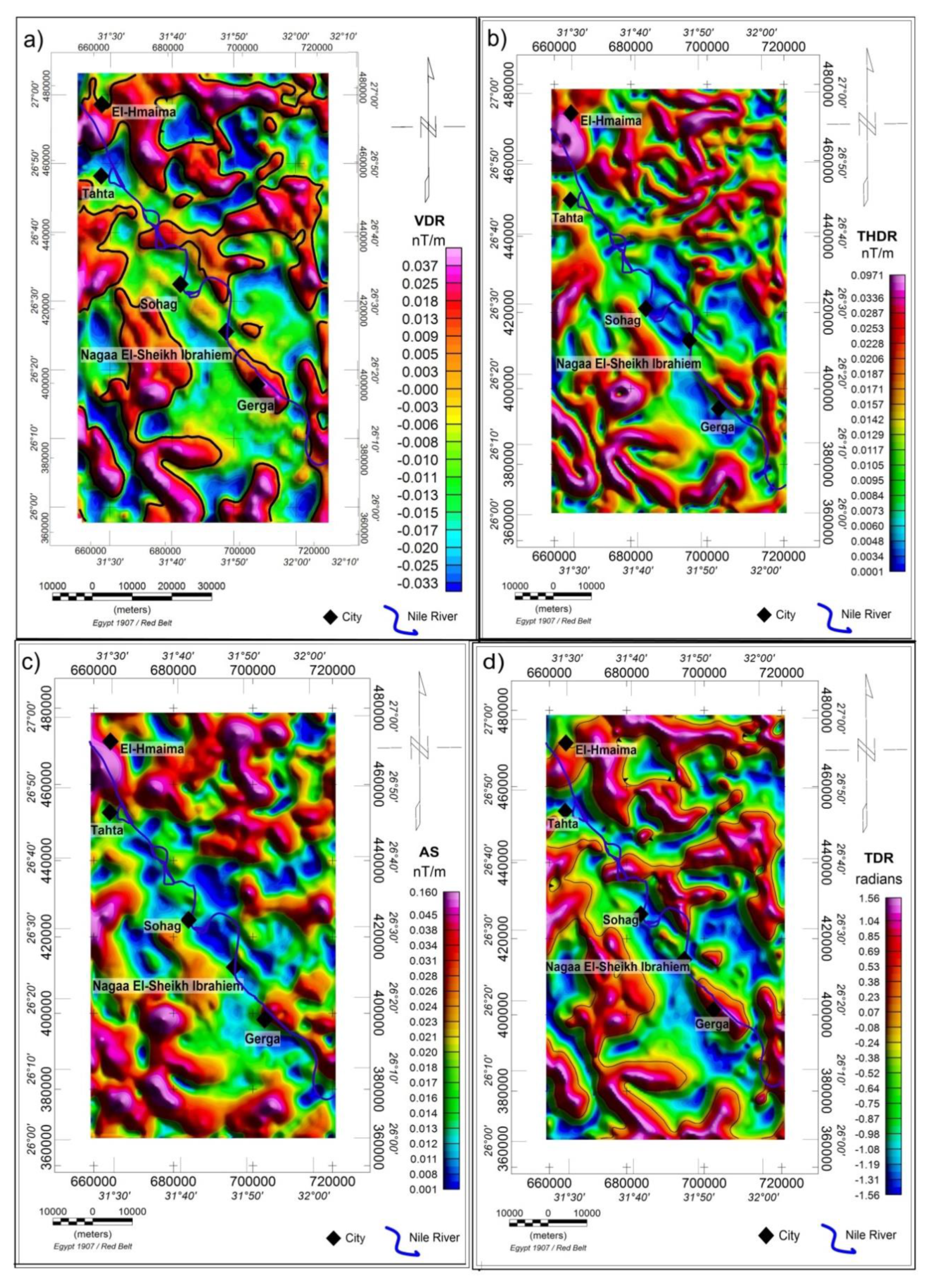
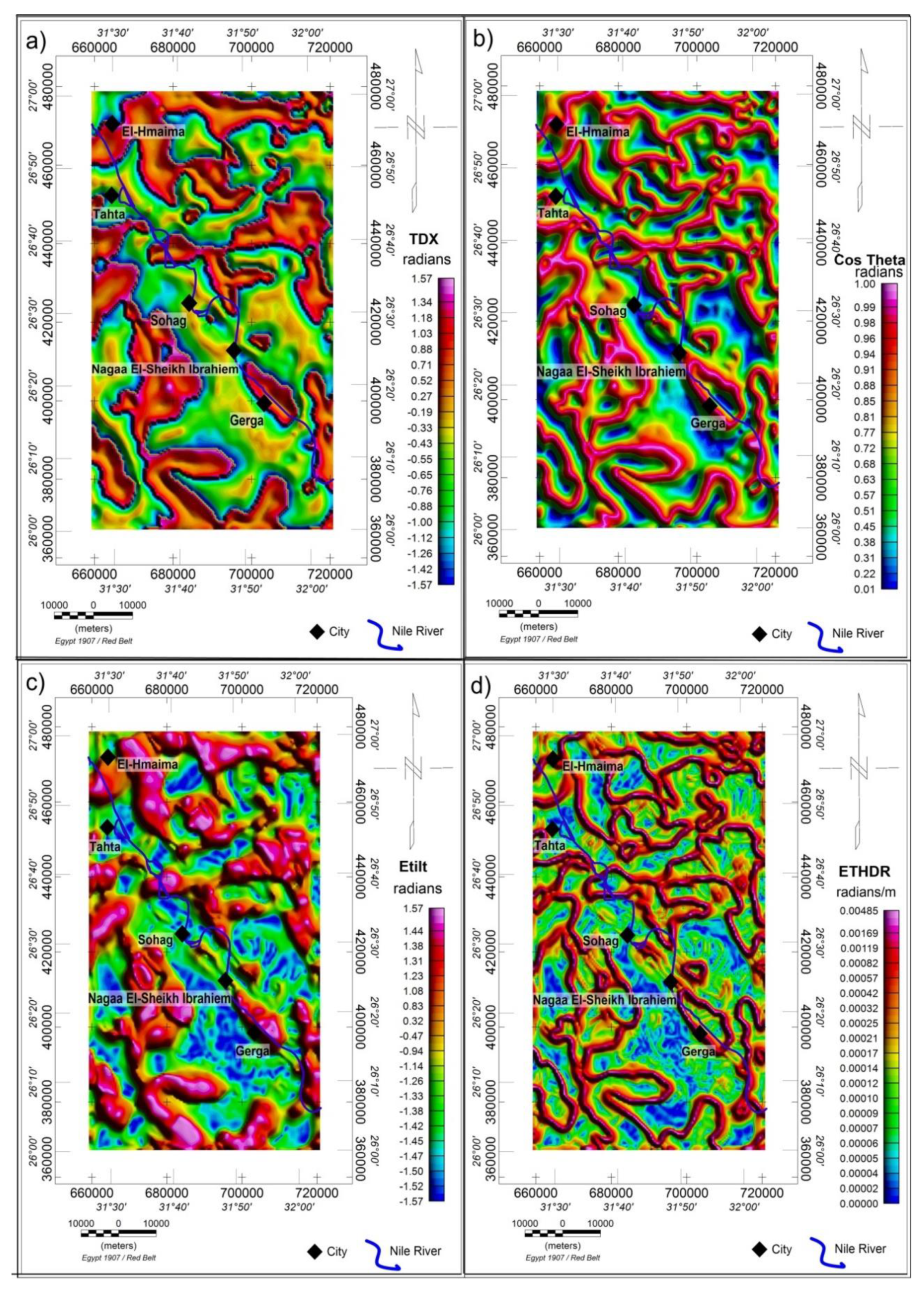
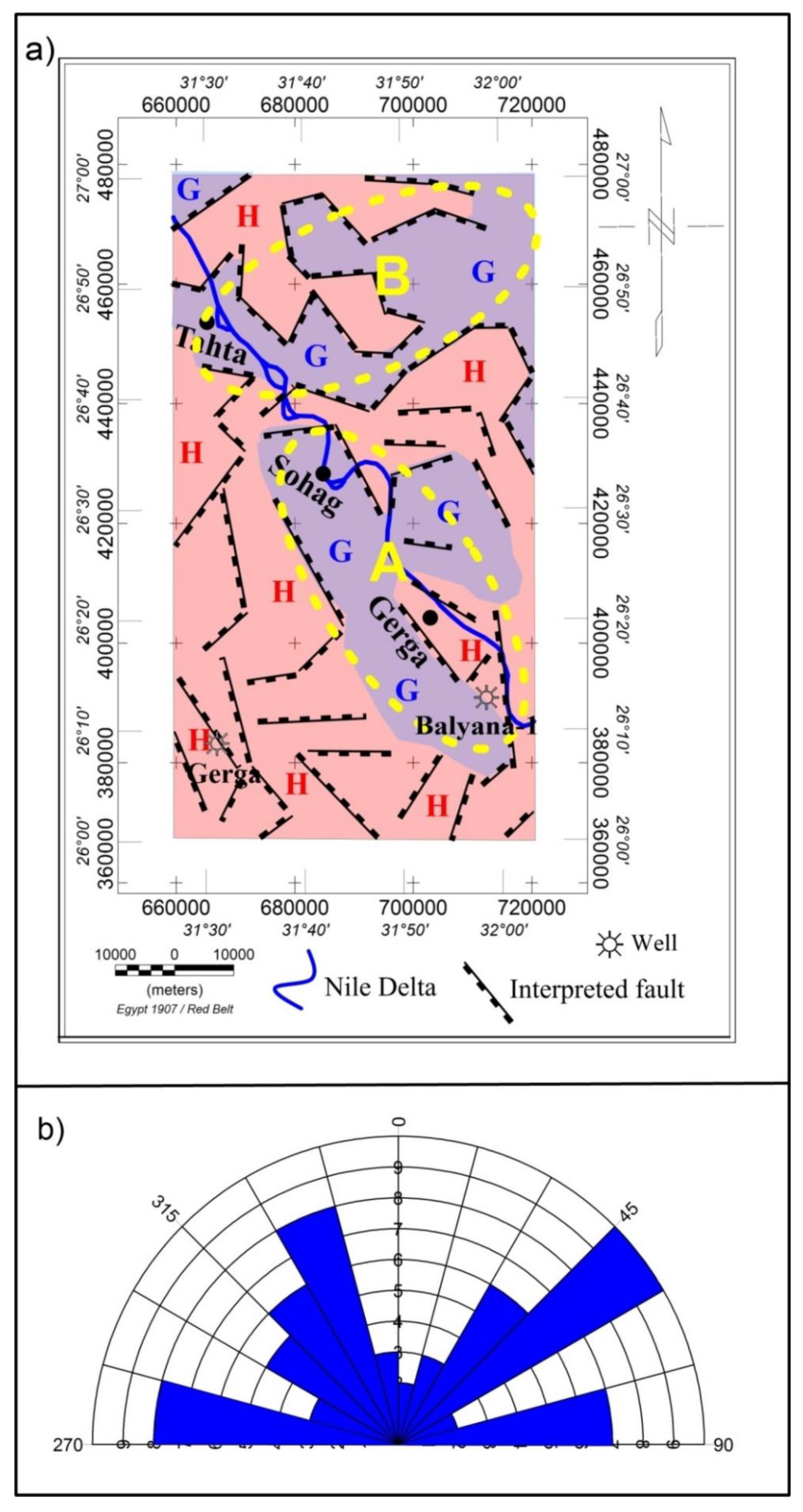
4. Results and Discussion

Derivative based methods are considered a fast means for processing magnetic grids and providing accurate information about structural settings, tectonic trends, and depths. However, the complexity of the structural situation in the Sohag region makes it necessary to apply an integrated approach using several edge detection techniques. Different filters were applied to the RTP magnetic data in this study in order to delineate the edges of magnetic sources for both shallow and deep structures (contacts, faults, and dykes). These filters include: VDR, THDR, AS, TDR (Figure 4a–d, respectively), TDX, Cos Theta, ETilt, and ETHDR (Figure 5a–d, respectively). It is worth to mention that the edges (fault/boundaries of the magnetic source) are defined by a contour value of 0 in VDR, TDR, and ETilt maps, whereas they coincide with the maxima (peaks) in other filters. The resultant maps show that these filters are highly suitable for mapping the basement structure and have distinct advantages over many conventional techniques. Several detailed anomalies can be observed and distinguished using these derivatives of weakly and strongly magnetized source bodies with comparable resolutions. These anomalies are not clearly being seen on the RTP magnetic map, especially in the northeastern section of the area. Zero contour lines of the VDR filter represent the location of the contacts/faults (Figure 4a). VDR, THDR, and TDR maps clarify that the northeastern and southwestern sections of the area are dissected by several shallow faults (VDR map), which can extend deeper to the basement (THDR and TDR maps). The AS map (Figure 4c) shows sundry magnetic bodies (intrusions/basement uplift) in the northern and southwestern sections. Although ETilt and ETHDR filters amplify the noise in the data, they nevertheless produced sharp gradients over the boundaries of the magnetic sources (Figure 5c,d).

High similarity can be observed between TDX, Cos Theta, ETilt, and ETHDR maps. Compared with the other derivative based filters, TDX, Cos Theta, ETilt, and ETHDR produce more detailed results for deeper magnetized structures and give a sharp response over the edges of the magnetic sources. The map created as the result of applying the ETHDR technique shows very sharp gradual anomalies concentrating over the edges of the bodies, and provides valuable information about structural settings from shallow and deep magnetic sources.

The ED technique was applied to the RTP aeromagnetic data with a window size of 15 × 15 and a maximum depth tolerance of 10%. The structural indexes SI = 0 (Figure 6a) was employed to locate contacts/faults with a small depth/throw ratio, and SI = 1 (Figure 6b) was used to detect dykes and/or faults with a large depth/throw ratio. A good clustering can be seen over the edges of magnetic sources (Figure 6a), showing a clear correlation with the results obtained from the edge detectors. Several dyke-shape bodies or basement intrusions can be observed in Figure 7b. The maps also show that the Nile River follows a structural path that is the result of deep and shallow faults during its historical evolution since the Late Miocene. The main tectonic trends of ED results are NW-SE, E-W, and NE-SW. The 3D ED solutions suggest depths to the basement surface varying from 500 to 4000 m as shown in Figure 6.

The structural features that control the accumulation of oil and gas are clarified in the detailed structural map, created by integrating the results obtained (Figure 7a). Only structural elements (faults, contacts, and intrusions) that were confirmed by several techniques were chosen in creating the structural map. The inferred map shows the existence of several faults causing a series of horsts (H) and grabens (G) in the study area. Two main basins (A and B) were determined representing the deepest area. The greatest thickness of sediments in basin A is located to the north of Gerga city, and for basin B it is in the northeastern section of the study area. We believe that these basins were formed as a result of down-faulted basement blocks. The deduced structural map also points out that the Nile River has changed its channel several times due to the existence of these faults, especially in the southern area of the study region near to Gerga city. The E-W (Tethyan-Mediterranean trend), N45-60E (Gulf of Aqaba trend), and N15-30W (Gulf of Suez trend) directions represent the main predominant tectonic trends in the area (Figure 7b). These trends correspond well with the known geological trends mentioned by [25], except the absence of a N-S trend. These tectonic events have not only influenced the basement topography, but also affected the subsequent sedimentation process and played a significant role in the evolution of the area. The results from the present study show that the positions of the drilled boreholes (Balyana-1 and Gerga) were not well chosen, as they were drilled in localities with high positive magnetic anomalies corresponding to thin sedimentary cover (Figure 2b).

5. Conclusions

Determining the edges of magnetic anomalies represents a fundamental stage in the structural interpretation of the subsurface using magnetic data. The increase in accuracy in edge location and the reduction of noise makes the use of edge detection techniques more common in geophysical exploration. The inferred structural map shows that the study area is affected by several faults that have formed alternative horst and graben structures. These faults influenced the Nile River channel, suggesting that the Nile River is tectonically controlled. The results show the dominance of three main tectonic trends in the investigated area: E-W, N45-60E, and N15-30W directions. The depths to the basement surface determined using 3D ED show that the depth varies from 500 to 4000 m. A seismic survey should be performed within the two main basins where the maximum thickness of sediments is available. Moreover, further exploratory drillings within the main basins are recommended to reassess the possibility of the presence of hydrocarbons. Finally, we conclude that the results of the present research provide structural information that constitutes an invaluable contribution to the process of gas and oil exploration in such a promising area.

References

1. Baranov, V. A new method for interpretation of aeromagnetic maps: Pseudo-gravimetric anomalies. Geophysics 1957, 22, 359–383. [Google Scholar] [CrossRef]
2. Arisoy, M.; Dikmen, Ü. Edge detection of magnetic sources using enhanced total horizontal derivative of the Tilt angle. Bull. Earth Sci. Appl. Res. Cent. Hacet. Univ. 2013, 34, 73–82. [Google Scholar]
3. Oruç, B. Edge detection and depth estimation using a tilt angle map from gravity gradient data of the Kozaklı-Central Anatolia region, Turkey. Pure Appl. Geophys. 2011, 168, 1769–1780. [Google Scholar] [CrossRef]
4. Verduzco, B.; Fairhead, J.D.; Green, C.M.; MacKenzie, C. New insights into magnetic derivatives for structural mapping. Lead. Edge 2004, 23, 116–119. [Google Scholar] [CrossRef]
5. Ardestani, V.E.; Motavalli, H. Constraints of analytic signal to determine the depth of gravity anomalies. J. Earth Space Phys. 2007, 33, 77–83. [Google Scholar]
6. Ferreira, F.J.F.; de Souza, J.; Bongiolo, A.B.S.; de Castro, L.G. Enhancement of the total horizontal gradient of magnetic anomalies using the tilt angle. Geophysics 2013, 78, J33–J41. [Google Scholar] [CrossRef]
7. Evjen, H.M. The place of the vertical gradient in gravitational interpretations. Geophysics 1936, 1, 127–136. [Google Scholar] [CrossRef]
8. Thompson, D.T. EULDPH: A technique for making computer assisted depth estimates from magnetic data. Geophysics 1982, 47, 31–37. [Google Scholar] [CrossRef]
9. Cordell, L.; Grauch, V.J.S. Mapping basement magnetization zones from aeromagnetic data in the San Juan basin, New Mexico. In The Utility of Regional Gravity and Magnetic Anomaly Maps; Hinzc, W.J., Ed.; Society of Exploration Geophysicists: Tulsa, OK, USA, 1985; pp. 181–197. [Google Scholar] [CrossRef]
10. Roest, W.R.; Verhoef, J.; Pilkington, M. Magnetic interpretation using the 3-D analytic signal. Geophysics 1992, 57, 116–125. [Google Scholar] [CrossRef]
11. Miller, H.G.; Singh, V. Potential field tilt—A new concept for location of potential field sources. J. Appl. Geophys. 1994, 32, 213–217. [Google Scholar] [CrossRef]
12. Fedi, M.; Florio, G. Detection of potential fields source boundaries by enhanced horizontal derivative method. Geophys. Prospect. 2001, 49, 40–58. [Google Scholar] [CrossRef]
13. Wijns, C.; Perez, C.; Kowalczyk, P. Theta map: Edge detection in magnetic data. Geophysics 2005, 70, L39–L43. [Google Scholar] [CrossRef]
14. Cooper, G.R.J.; Cowan, D.R. Enhancing potential field data using filters based on the local phase. Comput. Geosci. 2006, 32, 1585–1591. [Google Scholar] [CrossRef]
15. Phillips, J.D. Processing and Interpretation of Aeromagnetic Data for the Santa Cruz Basin-Patahonia Mountains Area, South-Central Arizona; U.S. Geological Survey Open-File Report 02-98; U.S. Geological Survey: Reston, VA, USA, 2002.
16. Oruç, B.; Keskinsezer, A. Structural setting of the northeastern Biga Peninsula (Turkey) from tilt derivatives of gravity gradient tensors and magnitude of horizontal gravity components. Pure Appl. Geophys. 2008, 165, 1913–1927. [Google Scholar] [CrossRef]
17. Marson, I.; Klingele, E. Advantages of using the vertical gradient of gravity for 3-D interpretation. Geophysics 1993, 58, 1588–1595. [Google Scholar] [CrossRef]
18. Cooper, G.R. Balancing images of potential-field data. Geophysics 2009, 74, L17–L20. [Google Scholar] [CrossRef]
19. Ibraheem, I.M.; Gurk, M.; Tougiannidis, N.; Tezkan, B. Subsurface investigation of the Neogene Mygdonian Basin, Greece using magnetic data. Pure Appl. Geophys. 2018, 175, 2955–2973. [Google Scholar] [CrossRef]
20. Reid, A.B.; Allsop, J.M.; Granser, H.; Millett, A.J.; Somerton, I.W. Magnetic interpretation in three dimensions using Euler deconvolution. Geophysics 1990, 55, 80–91. [Google Scholar] [CrossRef]
21. Zhou, W.; Nan, Z.; Li, J. Self-constrained Euler deconvolution using potential field data of different altitudes. Pure Appl. Geophys. 2016, 173, 2073–2085. [Google Scholar] [CrossRef]
22. Ravat, D. Analysis of the Euler method and its applicability in environmental investigations. J. Environ. Eng. Geophys. 1996, 1, 229–238. [Google Scholar] [CrossRef]
23. Ibraheem, I.M.; Elawadi, E.A.; El-Qady, G.M. Structural interpretation of aeromagnetic data for the Wadi El Natrun area, northwestern desert, Egypt. J. Afr. Earth Sci. 2018, 139, 14–25. [Google Scholar] [CrossRef]
24. Ghazala, H.H.; Ibraheem, I.M.; Haggag, M.; Lamees, M. An integrated approach to evaluate the possibility of urban development around Sohag Governorate, Egypt, using potential field data. Arab. J. Geosci. 2018, 11, 194. [Google Scholar] [CrossRef]
25. Said, R. The Geology of Egypt; Elsevier: Amsterdam, The Netherlands, 1962; 377p. [Google Scholar]
26. Mahmoud, F.A. Subsurface Geological Conditions, as Deduced from Gravity and Magnetic Data in the Area East of El-Balyana, Sohag, Egypt. Master’s Thesis, Geology Department, Faculty of Science, South Valley University, Sohag, Egypt, 1999. [Google Scholar]
27. El Emam, A.E. Geophysical Study around the Epicenter of Earthquake of 1 May 1999, Sohag, Western Desert, Egypt. Master’s Thesis, Mansoura University, Mansoura, Egypt, 2002; 158p. [Google Scholar]
28. Conoco. Geologic map of Egypt NG 36 NW Asyut (Scale 1: 500000); General Petroleum Company: Cairo, Egypt, 1987. [Google Scholar]
29. Issawi, B.; Francis, M.H.; Youssef, E.A.A.; Osman, R.A. The Phanerozoic geology of Egypt, a geodynamic approach. Egypt. Miner. Resour. Auth. 2009, 81, 192–200. [Google Scholar]
30. Said, R. Planktonic foraminifera from the Thebes formation, Luxor, Egypt. Micropaleontology 1960, 6, 277–286. [Google Scholar] [CrossRef]
31. Abdel Latif, A.; El Kashouty, M. Groundwater investigation in Awlad Salameh, Southern Sohag, Upper Egypt. Earth Sci. Res. J. 2010, 14, 63–75. [Google Scholar]
32. Ganoub El-Wadi Petroleum Holding Company. Geological Report of the Balyana-1 Well; The Egyptian General Petroleum Corporation: Cairo, Egypt, 1994. [Google Scholar]
33. El-Shazly, E.M.; Abdel-Hady, M.; El Ghawaby, H.; El Kassas, k.; Khawasik, S.M.; El Shazly, M.M.; Sanad, S. Geologic Interpretation of Land Satellite Images for West Nile Delta Area, Egypt; The Remote Sensing Center, Academy of Scientific Research and Technology: Cairo, Egypt, 1975; p. 38. [Google Scholar]
34. El-Shazly, E.M.; Abdel Hady, M.A.; El Kassas, I.A.; Salman, A.B.; El Amin, H.; El Shazly, M.M.; Abdel Megid, A.A. Geology of Kharga-Dakhla Oases Area, Western Desert, from Landsat-1, Satellite images, Nasa Landsat G-27930; Remote Sensing Center, Academy of Scientific Research and Technology: Cairo, Egypt, 1976; p. 64. [Google Scholar]
35. Youssef, M.I. Structural pattern of Egypt and its interpretation. AAPG Bull. 1968, 52, 601–614. [Google Scholar]
36. Ghazala, H.H.; Ibraheem, I.M.; Lamees, M.; Haggag, M. Structural study using 2D modeling of the potential field data and GIS technique in Sohag Governorate and its surroundings, Upper Egypt. NRIAG J. Astron. Geophys. 2018, 7, 334–346. [Google Scholar] [CrossRef]
37. Aero Service Division of the Western Geophysical Company of America. The Total Magnetic Intensity Map of Egypt. Scale of 1: 50,000; Aero Service Division of the Western Geophysical Company of America: San Diego, CA, USA, 1983. [Google Scholar]
Figure 1. Definition of the geometrical relationships between first-order vertical derivative (VDR), total horizontal derivative (THDR), analytic signal (AS), tilt angle (TDR), Theta map (Cos (θ)), and horizontal tilt angle (TDX).
Geosciences 09 00211 g001
Figure 2. (a) Location map of Sohag sector, (b) Shuttle Radar Topography Mission (SRTM) map, showing the elevation distribution of the study area, and (c) geologic map of the study area showing the main surface rock units and faults affecting the area (after [28]).
Geosciences 09 00211 g002
Figure 3. (a) Total magnetic intensity map of Sohag area and its surroundings. White dashed lines represent some flying transverse profiles (interval distance is 1.5 km), whereas white lines refer to some tie lines (interval distance is 5 km). (b) Reduction to the pole (RTP) magnetic map.
Geosciences 09 00211 g003
Figure 4. VDR (a), THDR (b), AS (c), and TDR (d) maps of the investigated area. The zero contour line is displayed on VDR and TDR maps to indicate the boundaries of causative magnetic sources.
Geosciences 09 00211 g004
Figure 5. TDX (a), Cos Theta (b), ETilt (c), and enhanced total horizontal gradient of tilt angle (ETHDR) (d) maps of the investigated area.
Geosciences 09 00211 g005
Figure 6. Superposition of the RTP magnetic map and the Euler deconvolution (ED) solutions for (a) structural index (SI) = 0 and (b) SI = 1.
Geosciences 09 00211 g006
Figure 7. Deduced structural map (a) and its rose diagram (b). H refers to horst or basement uplift and G refers to graben.
Geosciences 09 00211 g007