Article

Legacy Data: How Decades of Seabed Sampling Can Produce Robust Predictions and Versatile Products

1
Centre for Environment, Fisheries and Aquaculture Science (Cefas), Pakefield Road, Lowestoft NR33 0HT, UK
2
Geological Survey of Norway (NGU), Postal Box 6315 Torgarden, 7491 Trondheim, Norway
*
Author to whom correspondence should be addressed.
Geosciences 2019, 9(4), 182; https://doi.org/10.3390/geosciences9040182
Submission received: 22 March 2019 / Revised: 12 April 2019 / Accepted: 15 April 2019 / Published: 19 April 2019
(This article belongs to the Special Issue Geological Seafloor Mapping)

Abstract

:
Sediment maps developed from categorical data are widely applied to support marine spatial planning across various fields. However, deriving maps independently of sediment classification potentially improves our understanding of environmental gradients and reduces issues of harmonising data across jurisdictional boundaries. As the groundtruth samples are often measured for the fractions of mud, sand and gravel, this data can be utilised more effectively to produce quantitative maps of sediment composition. Using harmonised data products from a range of sources including the European Marine Observation and Data Network (EMODnet), spatial predictions of these three sediment fractions were generated for the north-west European continental shelf using the random forest algorithm. Once modelled these sediment fraction maps were classified using a range of schemes to show the versatility of such an approach, and spatial accuracy maps were generated to support their interpretation. The maps produced in this study are to date the highest resolution quantitative sediment composition maps that have been produced for a study area of this extent and are likely to be of interest for a wide range of applications such as ecological and biophysical studies.

1. Introduction

Continental shelf seas cover only ≈9% of the global seafloor [1], but are biologically productive, important for biogeochemical cycling [2], provide a wide range of resources and services to humanity, while at the same time experiencing increased human impacts [3]. Although these shallow seas (water depths generally less than 200 m) are relatively well researched, there is still a lack of detailed maps of seafloor sediments, substrates, habitats or even bathymetry. In Europe, the European Marine Observation and Data Network (EMODnet) was incepted in 2009 to provide a gateway to marine data across seven discipline-based themes, including geology. The EMODnet-Geology theme aims at providing harmonised information on marine geology in Europe. One of the central products is a seabed substrate map of European maritime areas [4]. This map was compiled by harmonising substrate information from more than 30 countries and consolidating the data into a single map product with three unified substrate classification schemes based on a modification of the Folk classification [5]. The Folk scheme classifies the sediment based on the sediment fractions of mud (grain size d < 63 μm), sand (63 μm ≤ d < 2 mm) and gravel (d ≥ 2 mm). Simplifying this scheme from the original 15 sediment classes to six and four sediment classes has allowed harmonisation of the European seabed substrate data into a unified substrate map. However, some differences cannot be resolved by nesting multiple classes within a broader class. For example, Folk [5] suggested a trace amount of gravel could be 0.01%, whereas in the current interpretation of “trace” applied by the British Geological Survey (BGS), a fraction of 1% gravel is applied [6]. Another example in the difference of sediment classification schemes has been the interpretation of the boundary between muddy sand and sand. The original definition of this boundary was based on a 9:1 ratio of sand to mud. This definition has been widely used, for example this is the approach taken by the EMODnet-Geology harmonised seabed substrate map. However, there have been other variations of this approach such as the BGS modified Folk diagram described in Long [6]. Here the sediments with less than 5% gravel are separated at a 4:1 ratio of sand to mud into the classes sand and muddy sand and Mud and sandy mud. This BGS modified Folk diagram has been widely adopted within the United Kingdom (UK), particularly in projects such as the UK Marine Protected Areas Programme [7].
While there are issues with comparing or harmonising maps derived from different classification schemes, the sediment data used to generate these maps often has more information about sediment grain size than simply class type. Half phi (φ) grain size distribution or the sediment fractions of mud, sand and gravel are commonly measured but rarely used for mapping. Information is lost in the process of simplifying the relative abundance of the grain size components to a sediment class. For example, within the Folk triangle the percentages of mud, sand and gravel vary within a sediment class by between 1% and 50% depending on the specific class [5]. While this may be acceptable for certain applications, benthic species assemblages do not fit neatly into different sediment classes [8] and these classes would not necessarily be appropriate to inform certain human activities (e.g., engineering work or aggregate extraction). Therefore, given the limitations of classified substrate maps, there is a need for alternative approaches, for example to relate to species occurrence data.
Recently, methods have been developed to produce quantitative sediment maps that make better use of the quantitative grain size data. Lark et al. [9] derived additive log-ratios of the three sediment fractions that could then be modelled across the UK continental shelf. These additive log-ratios were subsequently converted back into the relative sediment fractions thereby predicting the distribution of mud, sand and gravel at the seabed. This geostatistical approach also allowed the authors to express the local probability of each class. While those authors used cokriging, Stephens and Diesing [10] spatially predicted sediment composition with the Random Forest [11] algorithm based on additive log-ratios. Diesing [12] further highlighted the value of quantitative sediment maps by applying a similar method at a fine scale (10 m resolution) to predict sediment fractions across a site of approximately 15,000 km2. The layers produced by these models have already proved valuable in other work such as predicting the spatial distribution of organic carbon in surficial shelf sediments [13], quantifying and valuing organic carbon flows and stocks on the UK continental shelf [14], understanding variation in benthic pH gradients [15] and assessing North Sea demersal fisheries in relation to benthic habitats [16]. To further support this desire by scientists for regional continuous variables that are suitable for a range of applications, Wilson et al. [17] generated a range of layers including mud, sand and gravel fractions for the north-west European shelf. However, the resolution of these data was coarse at a spatial resolution of 0.125° by 0.125° (approximately 8 km by 13 km, although this varies with latitude), and the methodology considered each sediment component in isolation, which is not suitable for compositional data of this type [18].
In line with the efforts of EMODnet to unify outputs across Europe, and to apply state-of-the-art methods for modelling the distribution of sediments this study investigates the application of quantitative sediment composition models at the scale of a European sea-basin. Stephens and Diesing [10] developed these techniques to predict the fractions of the three sediment components of mud, sand and gravel for an area of UK and North Sea. While this approach was largely successful, producing an overall accuracy of 0.83, this initial study was limited in geographic extent and spatial resolution (500 m). Further, when considering the high groundtruth sample density in certain areas of their study area, such as the North Sea, it is likely that some pixels were attributed to more than one sample. As samples were randomly separated into training and testing datasets, this could have had the effect of inflating the reported accuracy.
Stephens and Diesing [10] also calculated prediction intervals to quantify the reliability of the predictions. However, as these related to the two additive log ratios, they remained somewhat difficult to interpret. Prediction error is likely to be concentrated in certain regions of a map, such as in areas of high complexity [19,20] or around poorly sampled features [21]. A number of papers have presented methods for representing the spatial distribution of map error [20,22], and incorporating these types of maps have been advocated elsewhere [23,24]. Here we present spatial accuracy maps to accompany the updated substrate maps, which will support the product’s use in future studies. The presented methodology draws upon the work of Comber et al. [22] by applying a weighting function to understand how accuracy varies across the study site. The objectives of this study are therefore to provide high-resolution (7.5 arc seconds or approximately 130 m by 230 m) spatial models of sediment composition in continuous and classified form, accompanied with maps of spatially-explicit map accuracy/error and covering large parts of the north-west European continental shelf.

2. Materials and Methods
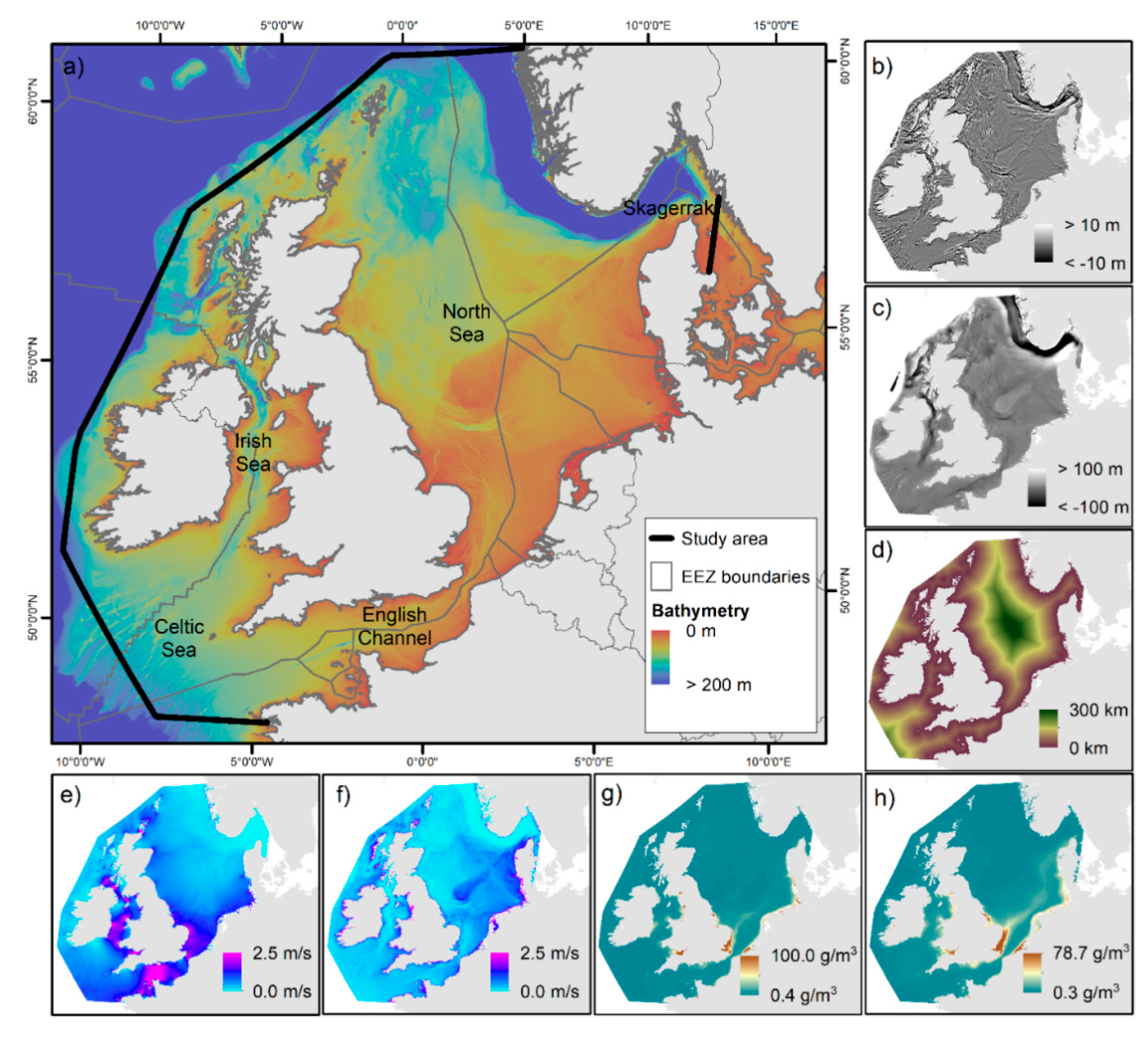
2.1. Study Area

The study area focusses on the north-west European continental shelf and includes the North Sea, Irish Sea, Celtic Sea, English Channel and Skagerrak (Figure 1a). This includes areas within the national maritime boundaries of Belgium, Denmark, France, Germany, Netherlands, Norway, Republic of Ireland, Sweden and the United Kingdom and Channel Islands.

2.2. Substrate Observations

Seabed samples were collated from several sources including national marine and geological institutes (Supplement S1). Some of these sources contained duplicate samples, but once these were removed the sample data downloaded from various sources consisted of approximately 68,000 samples where particle size distribution data existed. However, it was necessary to filter the data to remove potentially problematic samples, such as those where the reported sum of the percentages of mud, sand and gravel did not equal 100%. Samples collected prior to 1990 were also discarded, as these records may have imprecise positioning prior to the adoption of Global Positioning System. Inadequately recorded metadata meant that for many samples there was no information about how the grain size percentages were measured. Based on the disproportionate number of samples that were recorded with grain size percentages that were in round numbers (such as 50% sand/50% mud or 25% gravel/75% sand) it is likely that the fractions reported for these samples were estimated rather than analysed quantitatively. Commonly occurring fractions that were suspected of not being quantitatively measured were also discarded from analysis.
The density of samples varied considerably across the study site. As would be expected, areas near the coast were typically sampled at a higher density than those in deep environments and near the edge of the continental shelf. In areas of high sample density, it was common to have more than one sediment sample per unit of analysis (i.e., the spatial resolution of pixels used as predictor variables). Where this occurred, an average of the percentages of mud, sand and gravel was calculated to produce one set of fractions that was representative of that pixel. This resulted in a total sediment sample dataset of 45,761 samples.
The mud, sand and gravel fractions are compositional data, i.e., the sum of these fractions must equal 1 (or 100%) with each fraction constrained between 0 and 1. Therefore each component should not be considered in isolation from the others. We follow the recommendations of Aitchinson [18] and transform the data onto the additive log-ratio (ALR) scale where they can be analysed as two continuous, unconstrained response variables which assume any value. ALR tranformations are undefined if any observed value is zero. Therefore, we used the same rationale as Lark et al. [9], and all zero fractions were changed to the lowest observed fraction in the groundtruth data (0.01). Here we have selected to use the gravel fraction as the denominator of the log ratio, but it should be noted that the choice of variable does not affect the final outcome of the analyses [25].
a l r m =   log ( m u d g r a v e l ) = log ( m u d ) log ( g r a v e l )
a l r s =   log ( s a n d g r a v e l ) = log ( s a n d ) log ( g r a v e l )
The two additive log-ratios alrm and alrs constitute two response variables and separate predictive models can be built for each individually.
The data were then split randomly into training and testing datasets based on a 67/33% split (i.e., 30,480 training observations and 15,281 testing observations).

2.3. Predictor Variables

Variables used in the model are summarised in Table 1 and displayed in Figure 1a–h. Predictor variables were informed by Stephens and Diesing [10] and selected based on what was observed to be important for explaining the distribution of sediments.
A bathymetry Digital Terrain Model (DTM) was downloaded from the EMODnet-bathymetry portal (http://www.emodnet-bathymetry.eu/) for the study area [26]. The EMODnet-bathymetry is available in the World Geodetic System 1984 and has a gridsize of 1/8 arc minutes * 1/8 arc minutes (equal to 7.5 arc seconds). This equates to approximately 155 m * 230 m (x * y) in the south of the study area and 116 m * 230 m in the north of the study area. All other predictor variables (see below) were resampled onto this same 7.5 arc seconds grid. Bathymetric position indices [27] were calculated from the bathymetry DTM at two neighbourhood sizes that were thought to capture the local and regional variation and were sufficiently distinct to have limited correlation.
Two components of the hydrodynamic regime acting on the seabed were modelled and included for analysis. These were the average current speed and the wave peak orbital velocity at the seabed. Current speeds were derived from a purpose-built TELEMAC2D model with a mesh spacing ranging from 0.5 km to 10.0 km depending on the proximity to coast. This was then interpolated to the same 7.5 arc seconds grid as the other data layers. Peak orbital velocity of waves at the seabed were derived from a European continental shelf model of peak wave height and period from 2001–2010. This was based on a grid spacing of approximately 11 km. Using the method of Soulsby [28], this peak wave height and period were combined with depth and interpolated to the bathymetric grid (further details for current speed and peak wave velocity in Supplement S2 in the supplementary material).
Suspended inorganic particulate matter [29] derived from satellite imagery were downloaded from the Copernicus marine portal (OCEANCOLOUR_GLO_OPTICS_L4_REP_OBSERVATIONS_009_081). Data were downloaded at a 4 km resolution as monthly averages between January 2003 and December 2017. Data were averaged across the 15 years for the summer months (June, July and August) and winter months (December, January and February) to produce two separate rasters. Pixels obscured by cloud cover were ignored from analysis so there is the potential for some bias introduced as turbidity may be associated with increased cloud cover and therefore underrepresented in the dataset. Values represent g/m3. Rasters were then interpolated to the same 7.5 arc seconds grid as the other data layers.
Euclidean distance to coast was calculated in ArcGIS and was expected to be an indicator of distance to sediment source. Stephens and Diesing [10] observed the importance of this layer as a predictor variable.

2.4. Modelling

The random forest prediction algorithm [11] was selected as the model for this analysis as it showed a high level of predictive accuracy in similar studies [10,12], and is commonly applied to various modelling domains [30,31]. Random forests can be used without extensive parameter tuning, can handle many predictor variables and are insensitive to the inclusion of noisy or irrelevant features. Random forest models were implemented with the randomForest package [32] in R [33]. Forests had 500 trees and all other model parameters were kept as default.
Fitted models were applied to predict two response variables (alrm and alrs) as rasters, based on the available predictor variables. To generate the raster predictions of the three sediment fractions (mud, sand and gravel), the two response variables were back-transformed using the additive log-ratios:
m u d =   e x p ( a l r m ) e x p ( a l r m ) + e x p ( a l r s ) + 1
s a n d =   e x p ( a l r s ) e x p ( a l r m ) + e x p ( a l r s ) + 1
g r a v e l = 1 ( m u d + s a n d )
Using the abundance of the three sediment fractions, any classification scheme based on mud, sand and gravel fractions can be applied to create a classified map. These include commonly used schemes such as the Folk 5, Folk 7 and Folk 16 classes (where the number reflects the total number of classes in the classification scheme including one class for hard substrate) used in EMODnet Geology [34] and the EUNIS Level 3 classification for broadscale sedimentary habitats based on the simplified Folk triangle [6].

2.5. Model Validation

The random forest algorithm implicitly carries out a form of cross-validation using the ‘out-of-bag’ (OOB) observations (i.e., the observations not included in each tree). In addition, the models are validated against the test set of observations. The performance is assessed by calculating the mean of the squared prediction error:
M S E y ^ =   1 n i = 1 n ( y i y ^ i ) 2
where y are observed and y ^ are predicted values. The ‘variance explained’ (VE) by the model is then calculated by taking the ratio of the MSE to the variance ( σ 2 ) of the observed values:
V E = 1 M S E y ^ σ y 2
Using the test sample data set, classification accuracy was measured based on the predicted sediment type versus the original sediment type using the EUNIS Level 3 broadscale sediment classes, Folk 5 and Folk 16 maps. From this the overall accuracy, user’s and producer’s accuracy were calculated from the confusion matrix.
To represent the spatial distribution of error for each of the three sediment fractions the local Root-Mean-Squared-Error (RMSE) was calculated across the site. To do this, the squared error of each test sample was calculated based on the difference between the observed and predicted sediment fraction. A smoothed surface of local RMSE was then generated using the Inverse Distance Weighted (IDW) technique in ArcGIS. Each pixels’ RMSE was determined based on the closest 50 points (up to a maximum distance of 200 km). A weighting power function was applied in the IDW tool (set at 0.3) so nearer points contributed more to the pixel than distant points. The number and maximum distance were selected to produce an error map that had full spatial coverage but was locally constrained where sufficient samples were present. This IDW function was applied using a 1000 m * 1000 m grid to simplify computer processing.
For the classified predictions spatial accuracy was calculated using a locally constrained confusion matrix. Here test samples were converted to a Boolean value based on whether they were correctly classified. The IDW technique was applied to calculate a local thematic accuracy value. As above, this was applied based on the closest 50 points (maximum distance of 200 km) with a weighting power function of 0.3. This IDW function was applied using a 1000 m * 1000 m grid to simplify computer processing.
A comparison of classified model outputs with the sediment classification map from Stephens and Diesing [10] was also performed. As the maps had different extents and resolutions, a fishnet grid of 1000 * 1000 points was overlaid on the study side. Points outside the shared map extent or over land were removed and the prediction from both maps were extracted at the location of each remaining point. The results of the comparison were reported as a confusion matrix and overall agreement between maps was also calculated. Both maps would contain error, so the purpose of a comparison was to understand to what degree the changes to input data affected the final predictions.

3. Results

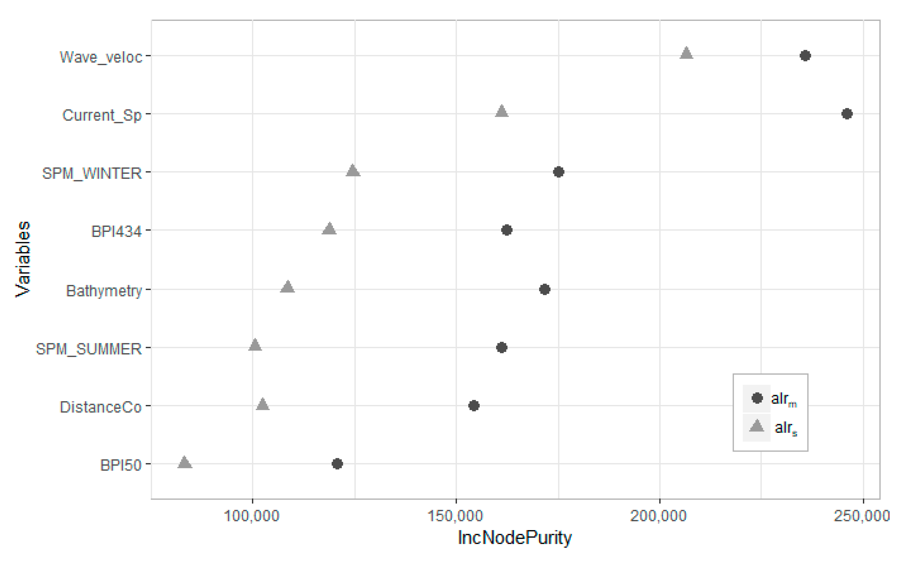
3.1. Features Importance

For both the alrm and alrs models the most important predictor variables were peak orbital wave velocity and mean tidal currents (Figure 2). All other variables were observed to contribute to the model, however, the relative importance changed for the alrm and alrs log-ratios.

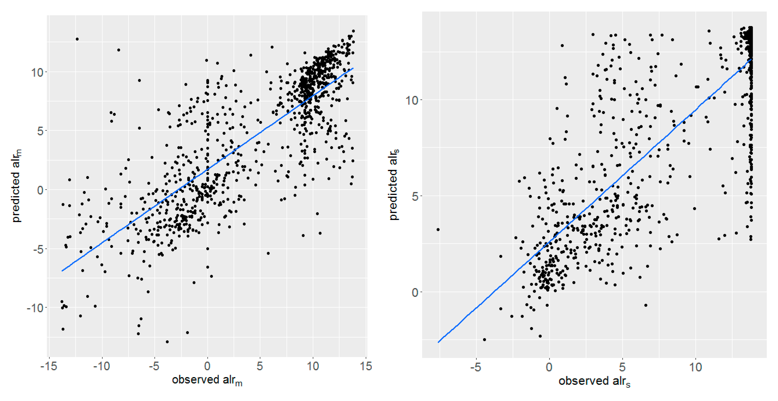
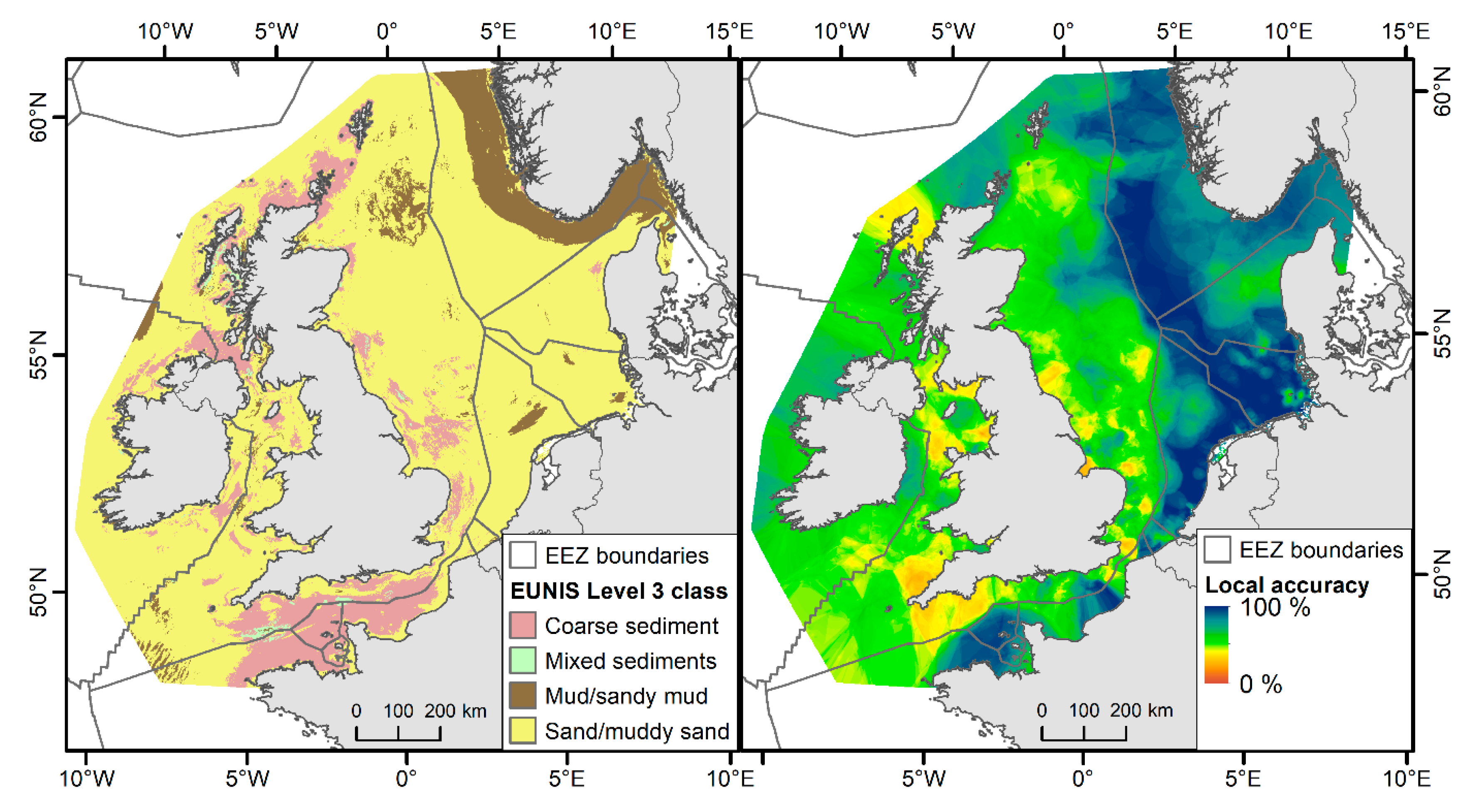
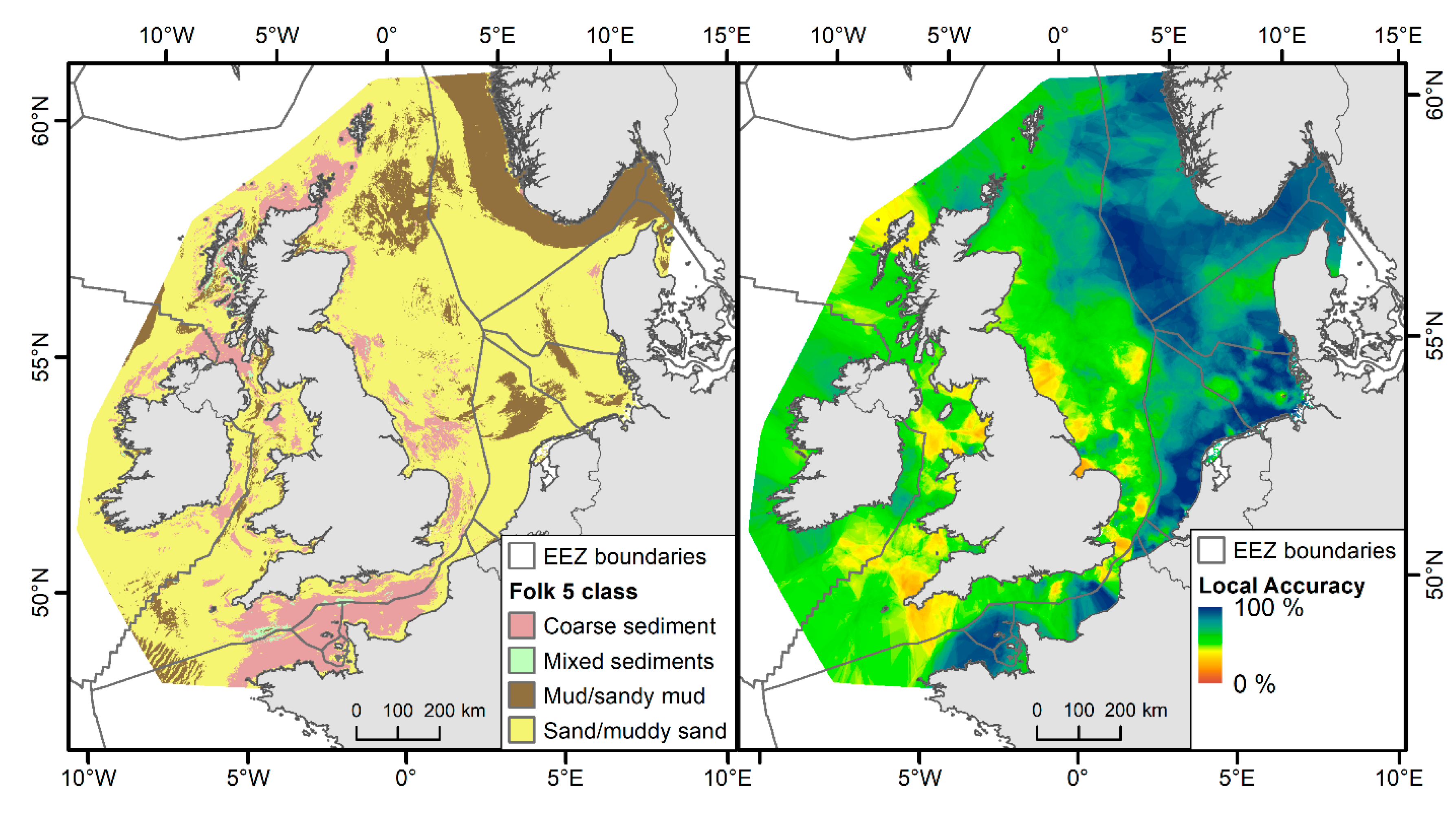
3.2. Model Validation

The model validation statistics (Table 2) indicate that the variance explained by the predictive models were approximately 63% for alrm and 68% for alrs. Figure 3 shows the observed versus predicted values for a random subset of the test samples for alrm and alrs. The plots show that there is considerable variation that was not explained by the models.
Of the three classification schemes applied the EUNIS Level 3 map was the most accurate with an overall accuracy of 77.5%, as opposed to 74.1% and 58.8% accuracy for Folk 5 and Folk 16 respectively (Table 3). The three confusion matrices show how the class accuracy is highly variable between classes. For example, in the EUNIS Level 3 map ‘Sand/muddy sand’ was the most widespread sediment type and was the most accurately mapped, with a user’s accuracy of 79.2%. For the same map the lowest classification accuracy was the class ‘mixed sediments’ (user’s accuracy of 49.6%) which was also the least sampled class. By comparison, the user’s accuracy values for the Folk 16 map were relatively low. Of the 15 sediment classes only four achieved a user’s accuracy of >50%. Yet, because this included the three most sampled classes, ‘muddy sand’, ‘sand’ and ‘sandy mud’ which totalled 73.8% of the samples this contributed to the overall accuracy being 58.8%. This sampling bias towards sandy sediments was further highlighted by comparing the producer’s and user’s accuracies within each classification scheme. The producer’s accuracy was higher than the user’s accuracy for the most sampled class in all three classification schemes (i.e., ‘sand/muddy sand’ within EUNIS Level 3 and Folk 5, and ‘sand’ in Folk 16), but for all other classes the producer’s accuracy was lower than the user’s accuracy (with the exception of the Folk 16 classes ‘gravelly sand’ and slightly gravelly muddy sand’).
Comparison of the classified outputs with previous work from Stephens and Diesing [10] indicate a high level of agreement between the predictions. Comparing the EUNIS Level 3 maps, which were the most accurate, where the two studies shared a similar extent the overall agreement between the maps was 78.1% (Table 4). However, map agreement was not consistent between the classes. Of the points classed as ‘sand/muddy sand’ in the updated sediment map 81.1% were given the same classification in the Stephens and Diesing [10] map. This compares with only 1.8% agreement for points classed as ‘mixed sediments’, which was the least widespread class.

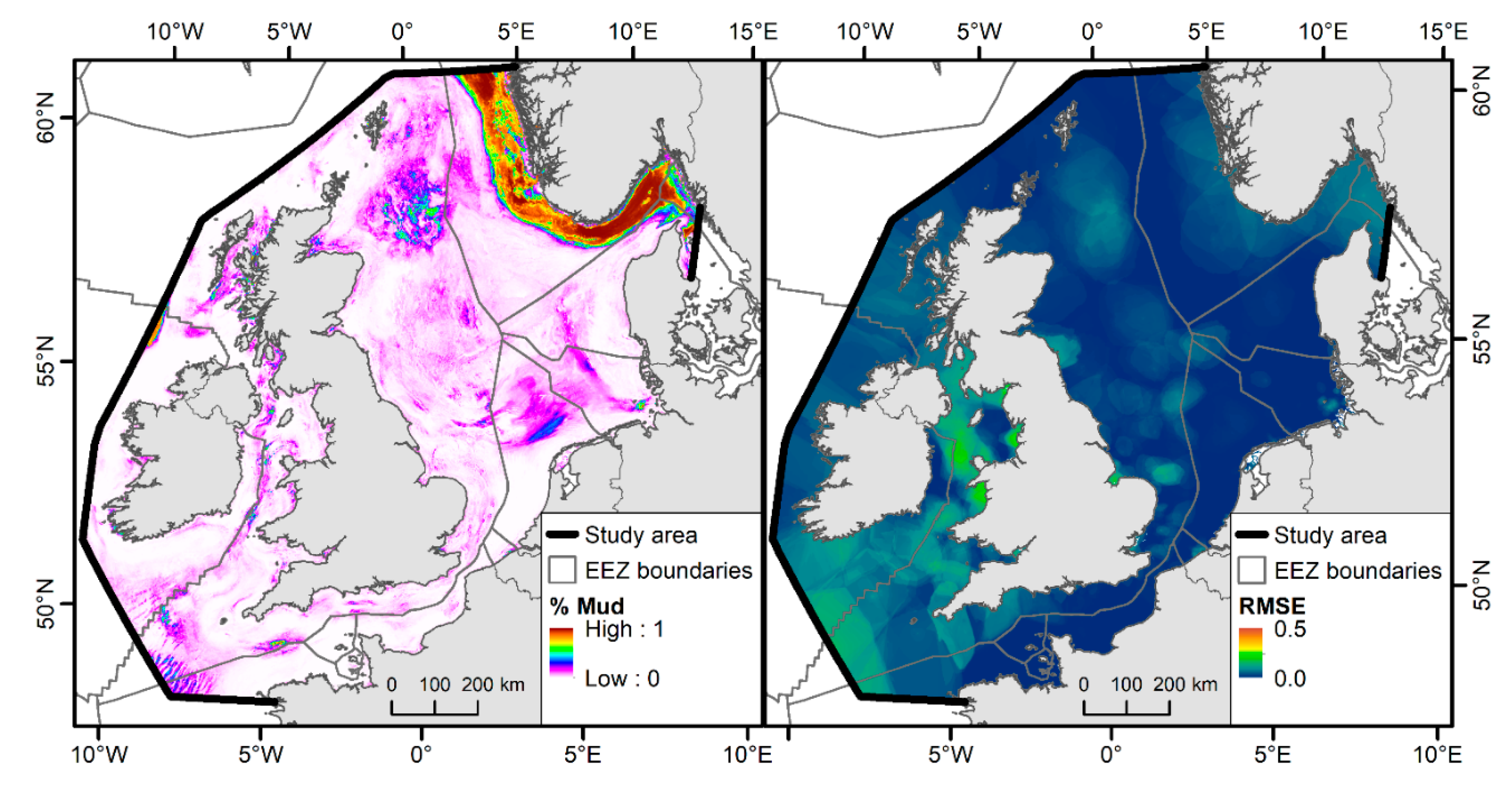
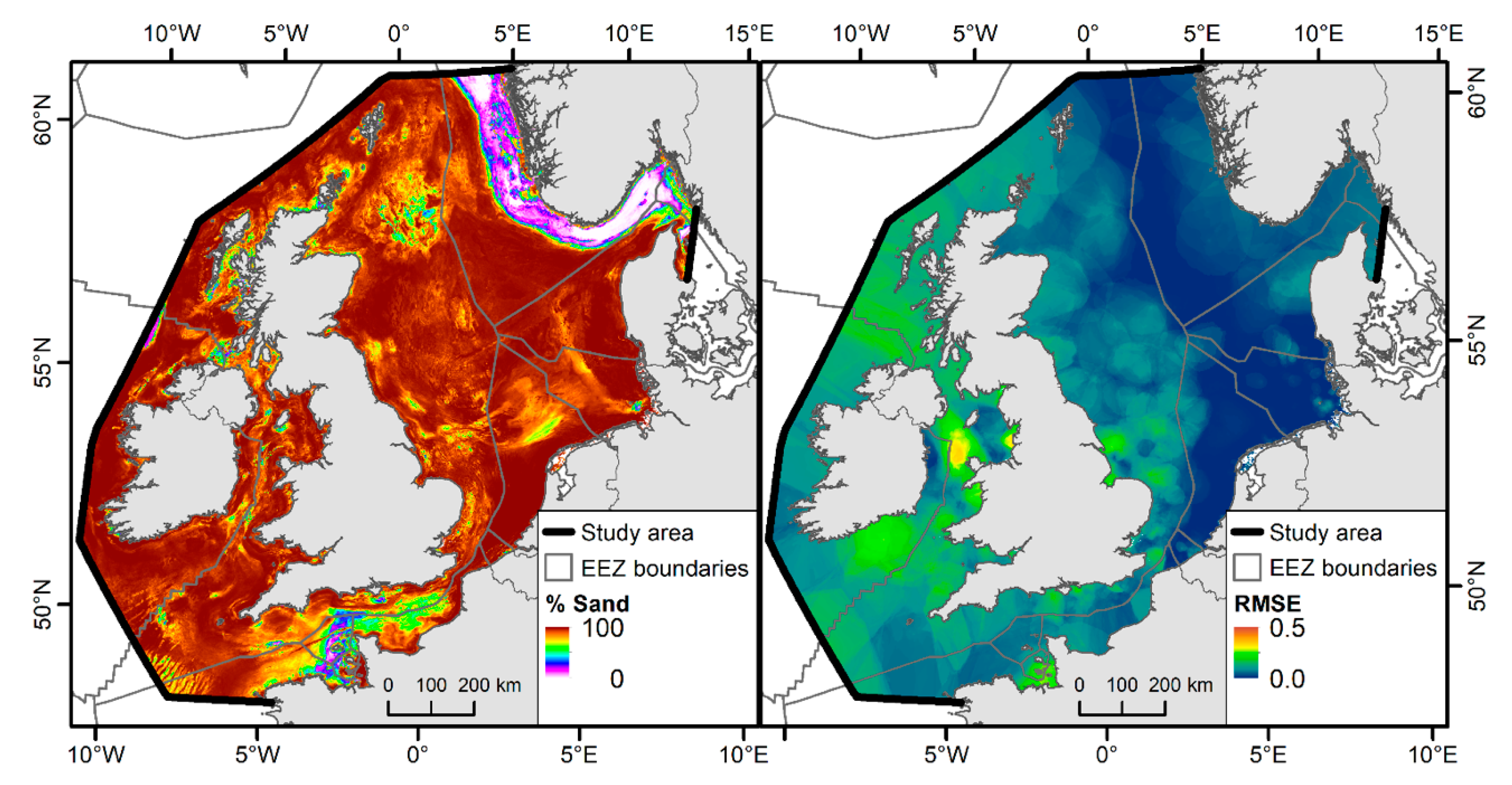
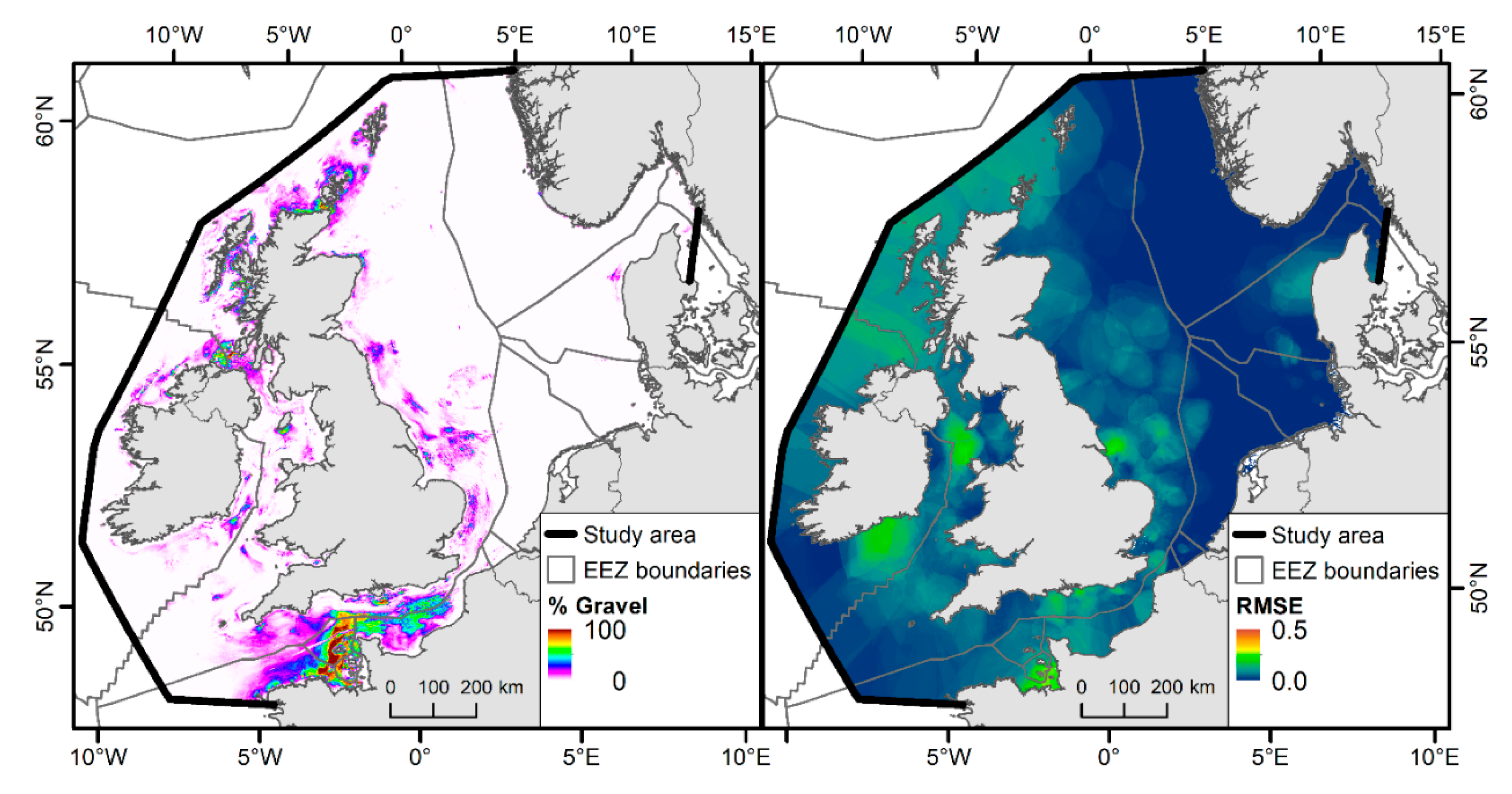
3.3. Sediment Composition

The predicted spatial distribution of the sediment fractions (mud, sand and gravel) are shown in Figure 4, Figure 5 and Figure 6 alongside the local RMSE for each sediment fraction. Sand was the most widespread sediment type. The mud fraction was prevalent in deeper areas such as the Norwegian Trough and, to a lesser extent, intra-shelf basins. Areas of high gravel fraction were predicted in the English Channel and other areas that experience high current speeds. For each sediment fraction the error associated with that prediction varied spatially across the study site. For example, while the predicted fraction of sand was high across most of the study site, error was particularly concentrated around the Irish sea and near the coast (Figure 5). The distribution of map error, as measured by local RMSE, is different for the three sediment fractions, however, they all indicate that the North Sea is an area of higher accuracy.
The classified maps, presented in Figure 7, Figure 8 and Figure 9, simplify these fractions into three commonly used classification schemes. The EUNIS Level 3 and Folk 5 predictions are generally similar, with the only difference being that Mud/sandy mud is more extensive in the Folk 5 classified map. These differences are most evident in the Fladen Grounds off eastern Scotland, the Oyster Ground north of the Netherlands and the Irish Sea. However, there is variation in local accuracy between the two schemes, most notably around the Fladen Grounds where the Folk 5 map has higher accuracy. The Folk 16 map is more detailed, with sand, muddy sand and sandy mud the most widespread sediment classes. However, the increased specificity resulted in lower local accuracies around the majority of the study area.

4. Discussion

The maps produced in this study are to date the highest resolution (7.5 arc seconds) quantitative sediment maps that have been produced at the scale of a sea-basin. Previous studies by Stephens and Diesing [10] and Wilson et al. [17] generated sediment predictions at 500 m and 0.125° resolution respectively. Increased resolution was possible due to improvements in the resolution of predictive layers available such as the tidal currents TELEMAC2D model and bathymetry layers available through the EMODnet project. Not only did an increased resolution bathymetry layer result in more detailed derivative layers but also, peak orbital velocity of waves at the seabed improved as the formula to calculate this from peak wave height and period requires depth to be known for each pixel. The two most important variables in both the alrm and alrs models were mean tidal current velocity and peak orbital velocity of waves at the seabed (Figure 2), both of which were modelled from new data that had a finer resolution. The extent of the study was also increased compared to Stephens and Diesing [10], including areas of the continental shelf around Ireland, northern Scotland, the Norwegian Trough and the Skagerrak. Regional maps such as these avoid the inevitable artefacts that occur at the borders between different datasets, national boundaries or study area [4,35]. These are typically a result of maps derived from different datasets or under different methods. Where the response variable is categorical only, as is generally the case, map users have few options with how to dissolve these boundaries so as to reflect reality. However, continuous response variables like the mud, sand and gravel fractions produced using this method may provide a useful tool to resolve these border issues. For example, areas of overlap could inform some degree of calibration factor to apply to one dataset or the other.
Increasing the resolution resulted in an overall accuracy of 78% for the EUNIS Level 3 map, which is less than the accuracy of 83% Stephens and Diesing [10] reported for their equivalent model. The independent test data indicated that approximately 60% and 63% of the variability was explained for the alrm and alrs respectively, which is also less than the 66% and 71% explained by Stephens and Diesing’s models. However, based on the number of sediment samples used by Stephens and Diesing [10] and the resolution of their study it appears that there may have been instances with multiple samples per pixel. This might have had the effect of artificially inflating the reported accuracy. As seen in Table 4, there was a high level of agreement between the two studies, but this was primarily for the ‘sand/muddy sand’ class, and caution should be taken when interpreting the extent of the other classes, in particular the ‘mixed sediments’ class.
This study benefited from recent attempts to compile multiple sources into large datasets (e.g., [36,37]). However, some sources of data had limited or no metadata. Therefore, it was impossible to know which methods were used to measure the quantity of sediment components. For example, samples collected using a standardised methodology [38] would have provided the most suitable samples for this process. However, methods such as laser grain size analysis can produce differences compared with more traditional sieving techniques [39]. As a minimum requirement to be included, samples needed to have the quantities of mud, sand and gravel recorded and be collected post-1990. Further attempts were made to filter the data by removing samples that contained some commonly occurring rounded fractions (e.g., 25%, 50% and 100%). However, it is likely that some imprecisely measured samples were still retained. Further, other sources of groundtruth error such as locational error [40], changes to sediment type through time and differences in sampling gear may have also increased map error but are unknown without adequate metadata. This paper therefore highlights the value of analysing sediment samples using robust quantitative techniques and the need for adequate metadata to be recorded so data can be appropriately utilised in future studies. However, the mapped outputs are still of value, as they portray sediment composition quantitatively and with increased resolution. Further, as they are supported with spatially-explicit maps of error, the level of reliance on the maps can be varied depending on the local accuracy.
Should a certain level of generalisation be required we would suggest incorporating object-based image analysis [41] into the workflow. This was displayed in Diesing [12] where ‘noisy’ pixel-based predictions were generalised using a process of segmentation, into areas of homogenous attributes, and then averaging the prediction between pixels within that segment. While generalised maps may be simpler for end users to interpret, they may also conceal some of the variability of a prediction. ‘Noisy’ areas within a map, where neighbouring pixels have a high degree of variation, may be an accurate reflection of the environment (e.g., high heterogeneity) or may be an artefact of the model (e.g., missing predictor variables or an overfitted model). Therefore, model generalisation may not always be desirable. For example, sediment fractions have proven more valuable than classified maps for understanding biologically meaningful species assemblages [8], and individual fractions may be particularly valuable for understanding certain sediment gradients, such as the organic carbon stocks [13].
It has been demonstrated that bedrock outcropping at the seabed can be reliably predicted [42,43,44]. Incorporating such information into basin-scale substrate maps would be a desirable goal in the future. However, several challenges must be met to make this happen: To our knowledge, maps of predicted bedrock occurrence do only exist for the UK continental shelf. Also, the existing maps have a much higher resolution (25 m) than the sediment predictions presented here. Finally, a framework must be developed that allows for expressing map accuracy or confidence when predictions have been made in different ways.
Increasing amounts and types of measured, modelled and remotely-sensed data have become available from the EMODnet and Copernicus data portals. At the same time, methods for quantitative spatial prediction and spatially-explicit error assessment continue to evolve. For example, a generic framework for predictive modelling of spatial and spatio-temporal variables using random forest has recently been presented [45]. We expect that similar products as those showcased here will ultimately become available for other sea areas within Europe. These will likely be of use for research as well as various applications such as habitat suitability modelling, nature conservation and marine planning among others.

Supplementary Materials

The following are available online at https://www.mdpi.com/2076-3263/9/4/182/s1. Supplement S1: Table summarizing sources of seabed sediment groundtruth data prior to filtering out problematic samples. Supplement S2: Further details on the preparation of mean tidal currents and peak wave velocities data for the UK continental shelf.

Author Contributions

Conceptualization, P.M. and M.D.; Methodology, P.M. and M.D.; Formal Analysis, P.M.; Data Curation, P.M. and J.A.; Writing—Original Draft, P.M., J.A. and M.D.; Funding Acquisition, M.D.

Funding

This study is part of the EU-funded EMODnet Geology project (EASME/EMFF/20I6/1.3.1.2—Lot 1/SI2.750862).

Acknowledgments

Thanks to the EMODnet-Geology partners who provided sediment sample data within the study area. Sediment sample data were also downloaded from the MOD web portal (https://mod.dnvgl.com/) in January 2018. This portal makes available monitoring data from the Norwegian continental shelf. The development of MOD is financed by Norsk Olje & Gass on behalf of the oil & gas industry in Norway. We would also like to thank David Haverson (Cefas) for providing access to tidal currents data for the European continental shelf.

Conflicts of Interest

The authors declare no conflict of interest.

Data Availability

Sediment observations and predictor variables are available from https://doi.org/10.14466/CefasDataHub.62. Data products presented in this study are available from https://doi.org/10.14466/CefasDataHub.63.

References

  1. Harris, P.T.; Macmillan-Lawler, M.; Rupp, J.; Baker, E.K. Geomorphology of the oceans. Mar. Geol. 2014, 352, 4–24. [Google Scholar] [CrossRef]
  2. Bauer, J.E.; Cai, W.-J.; Raymond, P.A.; Bianchi, T.S.; Hopkinson, C.S.; Regnier, P.A.G. The changing carbon cycle of the coastal ocean. Nature 2013, 504, 61–70. [Google Scholar] [CrossRef]
  3. Halpern, B.S.; Walbridge, S.; Selkoe, K.A.; Kappel, C.V.; Micheli, F.; D’Agrosa, C.; Bruno, J.F.; Casey, K.S.; Ebert, C.; Fox, H.E.; et al. A global map of human impact on marine ecosystems. Science 2008, 319, 948–952. [Google Scholar] [CrossRef]
  4. Kaskela, A.M.; Kotilainen, A.T.; Alanen, U.; Cooper, R.; Green, S.; Guinan, J.; Van Heteren, S.; Kihlman, S.; Van Lancker, V.; Stevenson, A.; et al. Picking up the pieces—Harmonising and collating seabed substrate data for European maritime areas. Geosciences 2019, 9, 84. [Google Scholar] [CrossRef]
  5. Folk, R.L. The distinction between grain size and mineral composition in sedimentary-rock nomenclature. J. Geol. 1954, 62, 344–359. [Google Scholar] [CrossRef]
  6. Long, D. BGS Detailed Explanation of Seabed Sediment Modified Folk Classification; MESH report; Joint Nature Conservation Committee: Peterborough, UK, 2006.
  7. Parry, M.E. Marine Habitat Classification for Britain and Ireland: Overview of User Issues; JNCC Report No. 529; Joint Nature Conservation Committee: Peterborough, UK, 2014.
  8. Cooper, K.M.; Bolam, S.G.; Downie, A.-L.; Barry, J. Biological-based habitat classification approaches promote cost-efficient monitoring: An example using seabed assemblages. J. Appl. Ecol. 2019. [Google Scholar] [CrossRef]
  9. Lark, R.M.; Dove, D.; Green, S.L.; Richardson, A.E.; Stewart, H.A.; Stevenson, A. Spatial prediction of seabed sediment texture classes by cokriging from a legacy database of point observations. Sediment. Geol. 2012, 281, 35–49. [Google Scholar] [CrossRef]
  10. Stephens, D.; Diesing, M. Towards quantitative spatial models of seabed sediment composition. PLoS ONE 2015. [Google Scholar] [CrossRef]
  11. Breiman, L. Random forests. Mach. Learn. 2001, 45, 5–32. [Google Scholar] [CrossRef]
  12. Diesing, M. Case Study: Quantitative Spatial Prediction of Seabed Sediment Composition; Cefas: Lowestoft, UK, 2015. [Google Scholar]
  13. Diesing, M.; Kröger, S.; Parker, R.; Jenkins, C.M.; Mason, C.; Weston, K. Predicting the standing stock of organic carbon in surface sediments of the North–West European continental shelf. Biogeochemistry 2017, 135, 183–200. [Google Scholar] [CrossRef]
  14. Luisetti, T.; Turner, R.K.; Andrews, J.E.; Jickells, T.D.; Kröger, S.; Diesing, M.; Paltriguera, L.; Johnson, M.T.; Parker, E.R.; Bakker, D.C.E.; et al. Quantifying and valuing carbon flows and stores in coastal and shelf ecosystems in the UK. Ecosyst. Serv. 2019, 35, 67–76. [Google Scholar] [CrossRef]
  15. Silburn, B.; Kröger, S.; Parker, E.R.; Sivyer, D.B.; Hicks, N.; Powell, C.F.; Johnson, M.; Greenwood, N. Benthic pH gradients across a range of shelf sea sediment types linked to sediment characteristics and seasonal variability. Biogeochemistry 2017, 135, 69–88. [Google Scholar] [CrossRef]
  16. van der Reijden, K.J.; Hintzen, N.T.; Govers, L.L.; Rijnsdorp, A.D.; Olff, H. North Sea demersal fisheries prefer specific benthic habitats. PLoS ONE 2018, 13, e0208338. [Google Scholar] [CrossRef]
  17. Wilson, R.J.; Speirs, D.C.; Sabatino, A.; Heath, M.R. A synthetic map of the northwest European Shelf sedimentary environment for applications in marine science. Earth Syst. Sci. Data Discuss. 2018, 10, 109–130. [Google Scholar] [CrossRef]
  18. Aitchison, J. The Statistical Analysis of Compositional Data; Chapman and Hall: London, UK, 1986; Volume 44, ISBN 00359246. [Google Scholar]
  19. Lucieer, V.L.; Lucieer, A. Fuzzy clustering for seafloor classification. Mar. Geol. 2009, 264, 230–241. [Google Scholar] [CrossRef]
  20. Foody, G.M. Local characterization of thematic classification accuracy through spatially constrained confusion matrices. Int. J. Remote Sens. 2005, 26, 1217–1228. [Google Scholar] [CrossRef]
  21. Mitchell, P.J.; Downie, A.-L.; Diesing, M. How good is my map? A tool for semi-automated thematic mapping and spatially explicit confidence assessment. Env. Model. Softw. 2018, 108, 111–122. [Google Scholar] [CrossRef]
  22. Comber, A.J.; Fisher, P.F.; Brunsdon, C.; Khmag, A. Spatial analysis of remote sensing image classification accuracy. Remote Sens. Environ. 2012, 127, 237–246. [Google Scholar] [CrossRef]
  23. Foody, G.M. Status of land cover classification accuracy assessment. Remote Sens. Environ. 2002, 80, 185–201. [Google Scholar] [CrossRef]
  24. Diesing, M.; Mitchell, P.J.; Stephens, D. Image-based seabed classification: What can we learn from terrestrial remote sensing? ICES J. Mar. Sci. 2016, 73, 2425–2441. [Google Scholar] [CrossRef]
  25. Pawlowsky-Glahn, V.; Olea, R.A. Geostatistical Analysis of Compositional Data; Oxford University Press: New York, NY, USA, 2004. [Google Scholar]
  26. EMODnet Bathymetry Consortium. EMODnet Digital Bathymetry (DTM 2016). Available online: http://portal.emodnet-bathymetry.eu/ (accessed on 30 March 2018).
  27. Lundblad, E.R.; Wright, D.J.; Miller, J.; Larkin, E.M.; Rinehart, R.; Naar, D.F.; Donahue, B.T.; Anderson, S.M.; Battista, T.A. A Benthic terrain classification scheme for American Samoa. Mar. Geod. 2006, 29, 89–111. [Google Scholar] [CrossRef]
  28. Soulsby, R.L. Simplified Calculation of Wave Orbital Velocities; HR Wallingford Ltd.: Wallingford, Oxfordshire, UK, 2006. [Google Scholar]
  29. Gohin, F.; Bryère, P.; Griffiths, J.W. The exceptional surface turbidity of the North-West European shelf seas during the stormy 2013-2014 winter: Consequences for the initiation of the phytoplankton blooms? J. Mar. Syst. 2015, 148, 70–85. [Google Scholar] [CrossRef]
  30. Zhi, H.; Siwabessy, P.J.W.; Nichol, S.L.; Brooke, B.P. Predictive mapping of seabed substrata using high-resolution multibeam sonar data: A case study from a shelf with complex geomorphology. Mar. Geol. 2014, 357, 37–52. [Google Scholar] [CrossRef]
  31. Hasan, R.C.; Ierodiaconou, D.; Laurenson, L.; Schimel, A.C.G. Integrating multibeam backscatter angular response, mosaic and bathymetry data for benthic habitat mapping. PLoS ONE 2014, 9, e97339. [Google Scholar]
  32. Liaw, A.; Wiener, M. Breiman and Cutler’s Random Forests for Classification and Regression, R package version 4.6–14. 2015; 29.
  33. R Development Team R. A Language and Environment for Statistical Computing; R Foundation for Statistical Computing: Vienna, Austria, 2017. [Google Scholar]
  34. Populus, J.; Vasquez, M.; Albrecht, J.; Manca, E.; Agnesi, S.; Al Hamdani, Z.; Andersen, J.; Annunziatellis, A.; Bekkby, T.; Bruschi, A.; et al. EUSeaMap, a European Broad-Scale Seabed Habitat Map, EMODnet. 2017.
  35. Lacharité, M.; Brown, C.J.; Gazzola, V. Multisource multibeam backscatter data: Developing a strategy for the production of benthic habitat maps using semi-automated seafloor classification methods. Mar. Geophys. Res. 2017, 39, 307–322. [Google Scholar] [CrossRef]
  36. Cooper, K.M.; Barry, J. A big data approach to macrofaunal baseline assessment, monitoring and sustainable exploitation of the seabed. Sci. Rep. 2017, 7, 12431. [Google Scholar] [CrossRef]
  37. Valerius, J.; van Lancker, V.; van Heteren, S.; Leth, J.; Zeiler, M. Trans-National Database of North Sea Sediment Data; Federal Maritime and Hydrographic Agency (Germany): Hamburg, Germany; Royal Belgian Institute of Natural Sciences (Belgium): Brussels, Belgium; TNO (Netherlands): The Hague, The Netherlands; Geological Survey of Denmark and Greenland (Denmark): Copenhagen, Denmark, 2014. [Google Scholar]
  38. Mason, C. NMBAQC’s Best Practice Guidance. Particle Size Analysis (PSA) for Supporting Biological Analysis; National Marine Biological AQC Coordinating Committee, 2016. [Google Scholar]
  39. Konert, M.; Vandenberghe, J. Comparison of laser grain size analysis with pipette and sieve analysis: A solution for the underestimation of the clay fraction. Sedimentology 1997, 44, 523–535. [Google Scholar] [CrossRef]
  40. Mitchell, P.J.; Monk, J.; Laurenson, L. Sensitivity of fine-scale species distribution models to locational uncertainty in occurrence data across multiple sample sizes. Methods Ecol. Evol. 2017, 8, 12–21. [Google Scholar] [CrossRef]
  41. Blaschke, T. Object based image analysis for remote sensing. ISPRS J. Photogramm. Remote Sens. 2010, 65, 2–16. [Google Scholar] [CrossRef]
  42. Diesing, M.; Green, S.L.; Stephens, D.; Cooper, R.; Mellett, C.L.L. Semi-Automated Mapping of Rock in the English Channel and Celtic Sea; JNCC: Peterborough, UK, 2015; Volume 569.
  43. Downie, A.L.; Dove, D.; Westhead, R.K.; Diesing, M.; Green, S.L.; Cooper, R. Semi-Automated Mapping of Rock in the North Sea; JNCC: Peterborough, UK, 2016.
  44. Brown, L.S.; Green, S.L.; Stewart, H.A.; Diesing, M.; Downie, A.-L.; Cooper, R.; Lillis, H. Semi-Automated Mapping of Rock in the Irish Sea, Minches, Western Scotland and Scottish Continental Shelf; JNCC Report; JNCC: Peterborough, UK, 2017; p. 609.
  45. Hengl, T.; Nussbaum, M.; Wright, M.N.; Heuvelink, G.B.M.; Gräler, B. Random forest as a generic framework for predictive modeling of spatial and spatio-temporal variables. PeerJ 2018, 6, e5518. [Google Scholar] [CrossRef]
Figure 1. Study area and variables used to predict the distribution of seabed sediments. (a) Bathymetry. (b) BPI50 cells. (c) BPI434 cells. (d) Distance from coast. (e) Current speed. (f) Peak orbital velocity. (g) Summer—suspended inorganic particulate matter. (h) Winter—suspended inorganic particulate matter. See Table 1 for additional details.
Geosciences 09 00182 g001
Figure 2. Feature importance scores. The importance of predictor variables for both modelled log-ratios indicated by the random forest algorithm. The x-axis indicates the average decrease in node sum of squares when variable is used.
Geosciences 09 00182 g002
Figure 3. Observed versus predicted values for 1000 random test set observations.
Geosciences 09 00182 g003
Figure 4. Predicted distribution of mud and spatial distribution of error, represented as local RMSE.
Geosciences 09 00182 g004
Figure 5. Predicted distribution of sand and spatial distribution of error, represented as local RMSE.
Geosciences 09 00182 g005
Figure 6. Predicted distribution of gravel and spatial distribution of error, represented as local RMSE.
Geosciences 09 00182 g006
Figure 7. Predicted sediment class based on EUNIS Level 3 class definitions and the spatial distribution of accuracy.
Geosciences 09 00182 g007
Figure 8. Predicted sediment class based on Folk 5 sediment class definitions and the spatial distribution of accuracy.
Geosciences 09 00182 g008
Figure 9. Predicted sediment class based on Folk 16 sediment class definitions and the spatial distribution of accuracy.
Geosciences 09 00182 g009
Table 1. Predictor variables used to model the distribution of sediments.
FeatureDescriptionUnitInitial ResolutionSource
BathymetryBathymetry (water depth).m7.5”http://www.emodnet-bathymetry.eu/ [26]
BPI50Bathymetric position index at 50—pixel radii.m7.5”Calculated from bathymetry
BPI434Bathymetric position index at 434—pixel radii (approximately 100 km).m7.5”Calculated from bathymetry
Distance from coastEuclidean distance to coast.m7.5”Calculated
Current SpeedMean tidal current velocity.m/s0.5–10 kmSupplement S2
Orbital velocity at the seabedPeak orbital velocity of waves at the seabed.m/s11 kmSupplement S2
Suspended inorganic particulate matter-SummerSatellite derived estimate of the amount of inorganic particulate matter suspended in the water column. Mean of from the months of June, July and August.g/m34 kmhttp://marine.copernicus.eu/
Suspended inorganic particulate matter—WinterSatellite derived estimate of the amount of inorganic particulate matter suspended in the water column. Mean of from the months of December, January and February.g/m34 kmhttp://marine.copernicus.eu/
Table 2. Model performance measured using out-of-the-box cross-validation and independent test data set.
alrmalrs
Cross validation (OOB)
MSE17.8610.91
Variance explained63.31%68.09%
Test set
MSE18.1910.93
Variance explained62.98%68.00%
Table 3. Confusion matrices for the three classification schemes against the test sample set. (a) EUNIS level 3. (b) Folk 5. (c) Folk 16. Correctly classified samples are highlighted in grey.
(a) EUNIS Level 3ObservedUser’s Accuracy
Coarse sedimentMixed sedimentsMud/sandy mudSand/muddy sand
PredictedCoarse sediment18713124038671.7%
Mixed sediments3663131549.6%
Mud/sandy mud153653312475.3%
Sand/muddy sand1197350913937779.2%
Producer’s Accuracy60.0%8.3%35.6%94.6%Overall
77.5%
(b) Folk 5ObservedUser’s Accuracy
Coarse sedimentMixed sedimentsMud/sandy mudSand/muddy sand
PredictedCoarse sediment18713127035671.7%
Mixed sediments3663181049.6%
Mud/sandy mud6080118631772.2%
Sand/muddy sand11523061247819775.2%
Producer’s Accuracy60.0%8.3%47.0%92.3%Overall
74.1%
(c) Folk 16Observed
GravelGravelly mudGravelly muddy sandGravelly sandMudMuddy gravelMuddy sandMuddy sandy gravelSandSandy gravelSandy mudSlightly gravelly mudSlightly gravelly muddy sandSlightly gravelly sandSlightly gravelly sandy mudUser’s Accuracy
PredictedGravel10--1-1---20-----31.3%
Gravelly mud-----11--------0.0%
Gravelly muddy sand191310244274143-55212.6%
Gravelly sand64108344239331261626734-22159324.7%
Mud--2-69-4-1-72--378.4%
Muddy gravel-----1-1-1--1--25.0%
Muddy sand51124243457301127614184-2716253.6%
Muddy sandy gravel2-11---617-----33.3%
Sand2225693804213836487155183165-544802275.4%
Sandy gravel7019122-516894691-226159.8%
Sandy mud115-2521626157111247.1%
Slightly gravelly mud-4871-4313811-3410.0%
Slightly gravelly muddy sand20146931469655933923325-3122312.2%
Slightly gravelly sand----12----1----0.0%
Slightly gravelly sandy mud---------------NA
Producer’s
Accuracy
5.1%0.0%4.6%34.0%37.7%1.9%43.1%1.7%89.8%28.9%12.4%0.0%21.2%0.0%0.0%Overall Accuracy
58.8%
Total number of samples19575283130118352169435179661623458314691437
Table 4. Comparison of high-resolution map with sediment map from Stephens and Diesing [10]. Cells indicating map agreement are highlighted in grey.
High ResolutionSumWithin Class Agreement
Coarse SedimentMixed SedimentsMud/Sandy MudSand/Muddy Sand
Stephens and Diesing [10]Coarse sediment25,8941446107236,56064,97240.0%
Mixed sediments36667572511635.8%
Mud/sandy mud8581210947914,21025,75736.8%
Sand/muddy sand11,4089482992221,143236,49193.5%
Sum38,526367113,548272,638Overall Agreement
78.1%
Within class agreement67.2%1.8%70.0%81.1%

