Article

Developing an Optimal Spatial Predictive Model for Seabed Sand Content Using Machine Learning, Geostatistics, and Their Hybrid Methods

National Earth and Marine Observations Branch, Environmental Geoscience Division, Geoscience Australia, GPO Box 378, Canberra, ACT 2601, Australia
*
Author to whom correspondence should be addressed.
Geosciences 2019, 9(4), 180; https://doi.org/10.3390/geosciences9040180
Submission received: 1 March 2019 / Revised: 15 April 2019 / Accepted: 15 April 2019 / Published: 17 April 2019
(This article belongs to the Special Issue Geological Seafloor Mapping)

Abstract

:
Seabed sediment predictions at regional and national scales in Australia are mainly based on bathymetry-related variables due to the lack of backscatter-derived data. In this study, we applied random forests (RFs), hybrid methods of RF and geostatistics, and generalized boosted regression modelling (GBM), to seabed sand content point data and acoustic multibeam data and their derived variables, to develop an accurate model to predict seabed sand content at a local scale. We also addressed relevant issues with variable selection. It was found that: (1) backscatter-related variables are more important than bathymetry-related variables for sand predictive modelling; (2) the inclusion of highly correlated predictors can improve predictive accuracy; (3) the rank orders of averaged variable importance (AVI) and accuracy contribution change with input predictors for RF and are not necessarily matched; (4) a knowledge-informed AVI method (KIAVI2) is recommended for RF; (5) the hybrid methods and their averaging can significantly improve predictive accuracy and are recommended; (6) relationships between sand and predictors are non-linear; and (7) variable selection methods for GBM need further study. Accuracy-improved predictions of sand content are generated at high resolution, which provide important baseline information for environmental management and conservation.

1. Introduction

Seabed mapping and characterization utilize datasets that describe the physical form and composition of seabed features that, when integrated, contribute important baseline information to support evidence-based environmental management [1,2,3,4,5,6]. A key component in the integration of seabed mapping data is the development of models that predict the spatial distribution of seabed sediment types (i.e., mud, sand, and gravel content). Previously, predictions of seabed sediments have been generated [7,8,9,10] at regional and larger scales for the Australian margin (e.g., seabed sand content at 1000 m resolution [11] and 250 m resolution for the northwest region [12]). However, these predictions were based largely on bathymetry-derived variables (e.g., slope, relief) and other spatial measures (e.g., latitude, longitude) due to data availability at these scales [7,8,9,10].
Many environmental variables have been reviewed [5,13] for marine environmental modelling, including acoustic multibeam data and their derived variables. In contrast to the limited availability of predictive variables at regional and larger scales, with the increased application of high-resolution acoustic multibeam technologies to seabed mapping, usually more predictive variables are available at desired resolution at local scales such as for seabed sediment [1,2,3,4]. Thus, bathymetry and backscatter have been used to predict seabed sediment at local scales [14]. However, the backscatter-derived variables have been rarely used for producing sediment predictions at local scales [4]. Here, we utilize high-resolution acoustic multibeam data and seabed sediment samples for the Timor Sea region, northern Australia (Figure 1) [15,16,17], to test the usefulness of backscatter-derived variables in combination with bathymetry-derived variables for improving predictive accuracy and generating high resolution, spatially continuous predictions of seabed sediments.
To generate spatially continuous predictions, many statistical and mathematical techniques can be applied [18,19,20]. The accuracy of these predictions is crucial for evidence-based environmental management and conservation. To improve the accuracy of seabed sediment predictions, many methods have been tested and compared [7,8,9,21]. Due to their high predictive accuracy in data mining and other disciplines [22,23,24,25,26,27,28], a number of machine learning methods, including random forests (RFs) and generalized boosted regression modelling (GBM), were introduced to spatial statistics by combining them with commonly used geostatistical methods to predict the spatial distribution of seabed sediments [7,8,9]. Consequently, some novel and accurate hybrid methods of machine learning and geostatistics were developed [7,8,9,21]. Some of these methods have shown high predictive capacity not only in marine environmental sciences [29] but also in terrestrial environmental sciences [30,31,32,33]. More importantly these highly accurate methods (i.e., RF, GBM, and their hybrid methods with geostatistics) as well as the most commonly used geostatistical methods (i.e., inverse distance weighting (IDW) and ordinary kriging (OK)) have been implemented in an R computing package, spm [34], which provides useful tools for this study.
Variable selection is essential for developing an optimal RF predictive model [10,35,36] and is also essential for its hybrid methods [8,9,37,38]. Several variable selection methods (e.g., variable importance (VI), averaged VI (AVI), knowledge-informed AVI (KIAVI), Boruta [39] and regularized RF (RRF), and variable selection using RF (VSURF) [40]) were tested for RF [29,35,41], where predictive accuracy was used to determine the selection of each predictive variable; and AVI or KIAVI were recommended [29,35,41]. However, variable selection for generalized boosted regression modelling (GBM) is rarely addressed, although a variable selection method based on relative variable influence (RVI), which is similar to VI for RF [42], has been used for deriving a dataset in spm from a full dataset containing 50 predictive variables [29].
In this study, we apply advanced spatial predictive methods in spm to predict seabed sand content in the Timor Sea region of northern Australia, based on seabed samples, acoustic multibeam data, and their derived variables. To achieve this, we: (1) compared several variable selection methods for RF; (2) developed and applied a variable selection method for GBM; (3) compared the predictive accuracy of models based on RF and its hybrid methods with OK and IDW (i.e., RFOK and RFIDW), GBM, IDW, and OK; and (4) predicted sand content using the most accurate model and visually examined the spatially continuous predictions.

2. Materials and Methods

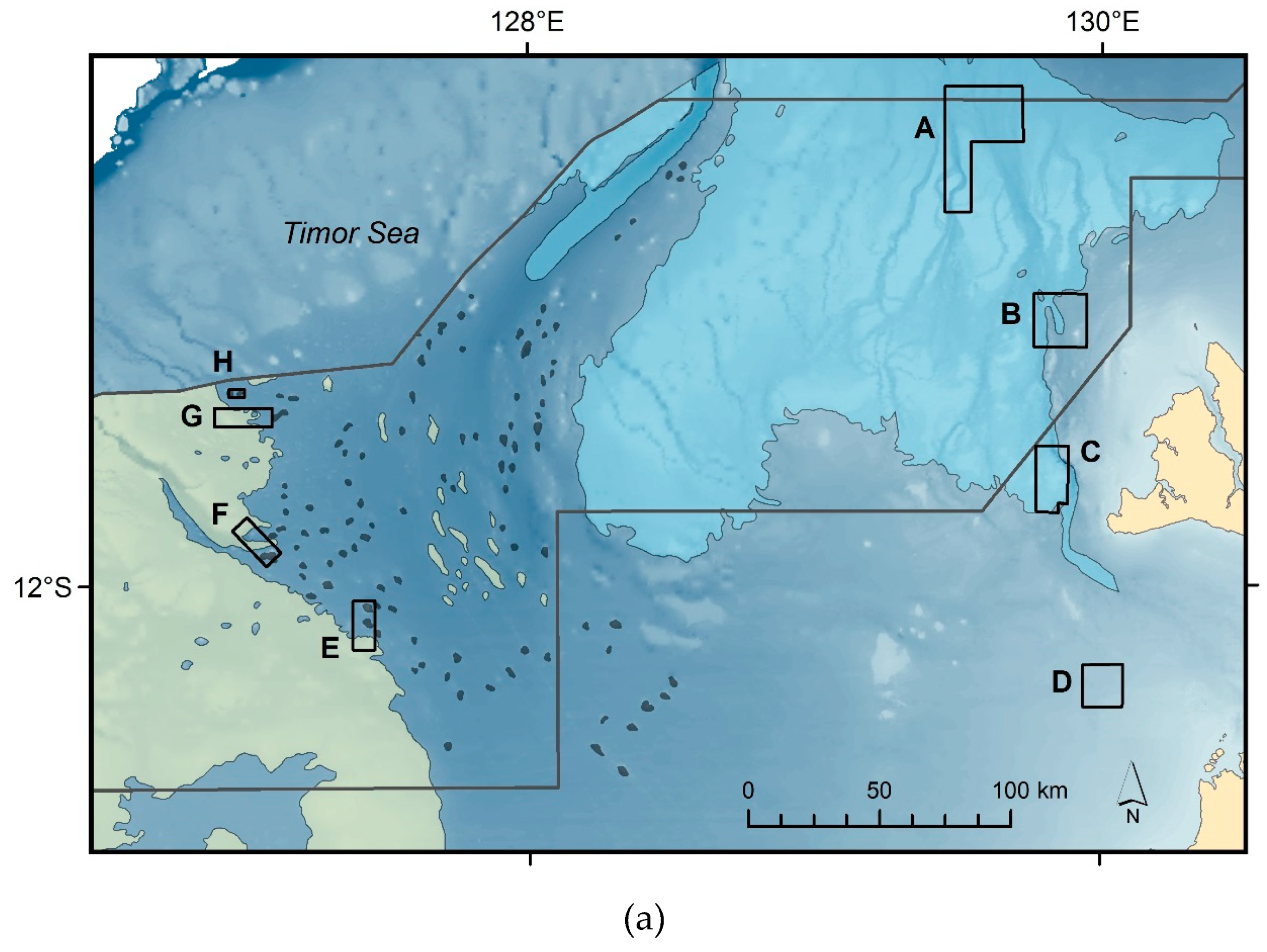
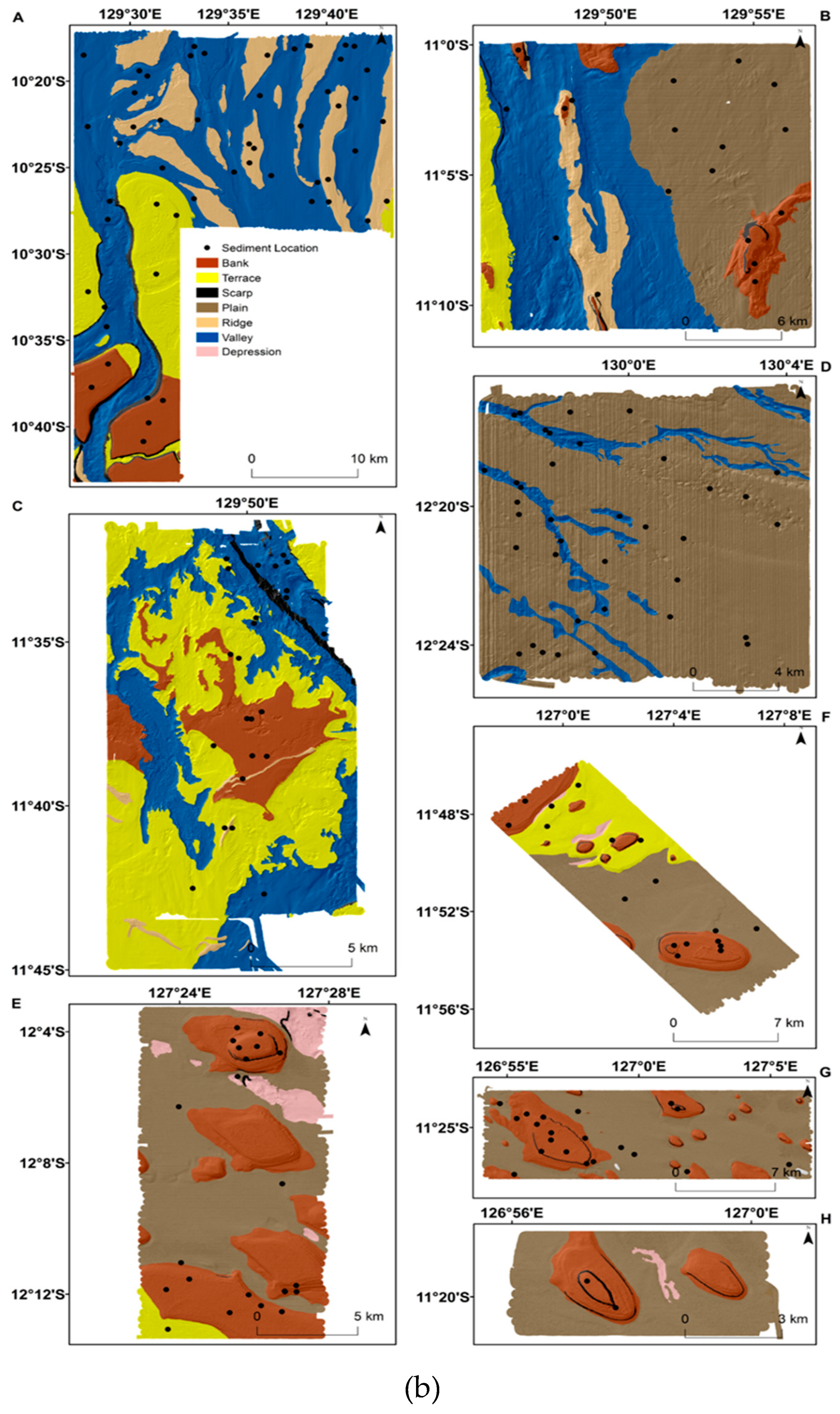
2.1. Study Region and Sediment Samples

The study region was located in the outer Joseph Bonaparte Gulf and Timor Sea offshore northern Australia. Here, the continental shelf is characterized by a spatially complex seabed of shallow carbonate banks and terraces separated by valleys and plains (Figure 1). Within this region, eight areas (A–H) were surveyed between 2009 and 2012 to acquire high-resolution bathymetry, acoustic backscatter data, and seabed samples [15,16]. Bathymetry and backscatter data were collected using a Kongsberg EM3002D 300 kHz multibeam sonar system and sediment samples collected using grab and gravity corer methods. Post-processing of bathymetry and backscatter data is detailed in post-survey reports [15,16,17], with resultant grids reduced to a common 10 m spatial resolution for this study. In survey areas A–D, sediment sampling sites were selected to represent all geomorphic seabed features across the range of mapped water depths. In the survey areas E–H, sampling sites were selected using a spatially-balanced random stratified method [15,16,17] and further detailed in subsequent studies [6,29,43,44]. In total, 195 seabed sediment samples were collected and processed in the laboratory using wet sieve separation to determine percentage gravel, sand, and mud content.
In this study, sand content data were used as a response variable. The sand content data are in percentage and provided in S1.

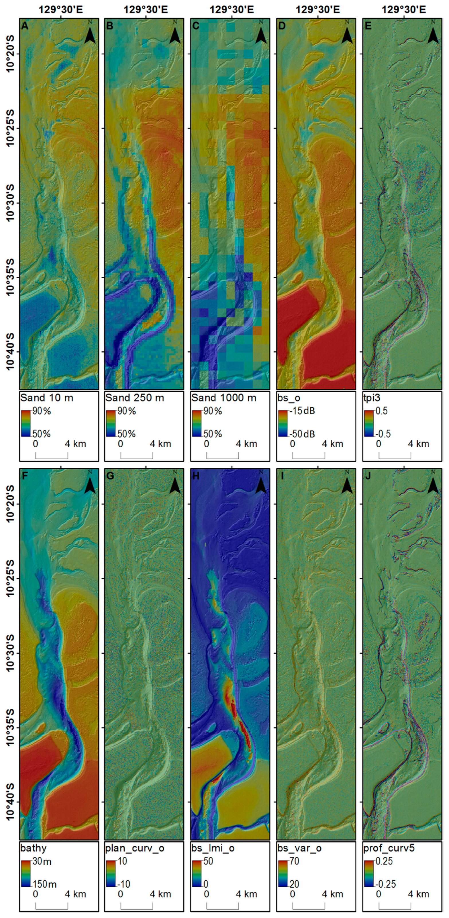
2.2. Predictive Variables

Following a preliminary analysis based on data availability and the relationships with seabed sediments [7,8,9,37,45,46], 77 predictive variables were acquired for this study. They were:
  • Two location variables: latitude (lat) and longitude (long),
  • Bathymetry (bathy),
  • Twenty-seven backscatter (bs) variables (bs10 to bs36): a diffused reflection of acoustic energy due to scattering process back to the direction from which it was generated, measured as the ratio of the acoustic energy sent to a seabed to that returned from the seabed, normalized to incidence angles between 10° and 36°,
  • Seventeen backscatter-derived variables from bs25 based on object and spatial windows (i.e., window size of 30, 50, and 70 m) approach:
    • bs_o,
    • homogeneity (bs_homo_o, bs_homo3, bs_homo5, and bs_homo7),
    • entropy (bs_entro_o, bs_entro3, bs_entro5, and bs_entro7),
    • local Moran I (bs_lmi_o, bs_lmi3, bs_lmi5, and bs_lmi7), and
    • variance (bs_var_o, bs_var3, bs_var5, and bs_var7).
  • Twenty-nine derived variables from bathy using object and spatial windows (i.e., window size of 30, 50, and 70 m) approach:
    • bathy_o,
    • lmi_o, lmi3, lmi5, lmi7,
    • topographic position index (tpi_o, tpi3, tpi5, and tpi7),
    • seabed slope (slope_o, slope3, slope5, and slope7),
    • planar curvature (plan_cur_o, plan_cur3, plan_cur5, and plan_cur7),
    • profile curvature (prof_cur_o, prof_cur3, prof_cur5, and prof_cur7),
    • topographic relief (relief_o, relief3, relief5, and relief7), and
    • seabed rugosity (rugosity_o, rugosity3, rugosity5, and rugosity7).
  • Distance to coast (dist.coast).
Acquisition and processing of multibeam bathymetry, backscatter, and their derived variables have been detailed in S2 and also described in previous studies [29,42,47]. All these variables were numerical and available for each grid cell at 10 m resolution in the eight study areas for generating the spatial predictions of sand content in this study. They were also available at the 195 sample locations for developing models to predict seabed sediments (S1).

2.3. Preliminary Selection of Predictive Variables

There were strong correlations among some predictive variables (e.g., lmio and lmi3, bs12 and bs13) based on Spearman’s rank correlation (ρ). The use of ρ was due to non-linear relationships between some variables. Amongst the highly correlated predictors (i.e., ρ ≥ 0.99), only the variable with the highest ρ with sand content was retained, leading to the overall retention of 49 variables. The inclusion of highly correlated variables (i.e., ρ < 0.99) were because they improved the predictive accuracy in previous studies [8,29,35,36,42]. The bs25 was used as it was the default backscatter predictor in Geoscience Australia (S2). As a result, in total 50 variables were used for this study (Table 1).

2.4. Predictive Methods

We used RF, RFOK, RFIDW, GBM, IDW, and OK (Table 2) to develop an optimal predictive model to predict sand content. For RFOK and RFIDW, firstly RF was applied to the data, then OK or IDW was applied to the residuals of RF. We also used the average of RFOK and RFIDW (RFOKRFIDW) to test if the predictive accuracy could be improved by model averaging.
R functions (i.e., idwcv, okcv, gbmcv, RFcv, rfokcv, rfidwcv, and rfokrfidwcv) that executed the above methods in spm [34] were used to develop models to predict the spatial distribution of seabed sediments. The default values of mtry, ntree, and node size in randomForest were often good options [23,48], which were also observed in studies in marine environmental sciences [8,42]; therefore, the default values were used for these parameters. The default values were used for relevant parameters in gbmcv.
The optimal parameters for IDW, OK, RFOK, and RFIDW were selected using the corresponding cross-validation functions (i.e., idwcv, okcv, rfokcv, and rfidwcv) in spm and summarized in Table 3. Since the sand content was percentage data, arcsine transformation needed to be used to normalize the data to meet the data normality requirement of OK. However, the implementation of arcsine transformation in okcv reduced the predictive accuracy in comparison with the default option (i.e., ‘none’ transformation), so the default option was used in this study. We also used the default parameters in Geostatistical and Spatial Analyst extensions in ArcGIS for IDW and OK as controls for comparison.

2.5. Variable Selection for Random Forest (RF)

Variable selection was based on a procedure developed for RF in previous studies [10,29,36,41,42], where the variables were selected based on variable importance and more importantly, on the accuracy of the resultant predictive model. The final selection of a predictive variable was based on its contribution to predictive accuracy (e.g., Figure 2a). That is, only those predictors that could improve the predictive accuracy were selected.
Five feature selection methods were used to select predictors in this study: (1) averaged variable importance (AVI), (2) Boruta, (3) knowledge-informed AVI (KIAVI) as detailed in previous studies [29,35,42], (4) recursive feature selection (RFE) [49], and (5) variable selection using RF (VSURF) [40]. The selection of these methods was based on previous studies [29,50]. Due to the randomness associated with the variable importance generated by the RF algorithm, the least important variable(s) may change with individual iterations; meanwhile correlated variables may also affect the order of the least important variable(s). To address this issue, a function, avi, in spm that is based on the R package ‘extendedForest’ [51], was used with 100 repetitions to stabilize the variable importance and to generate the average values of variable importance that were used to select the predictors. The process of variable selection using AVI and KIAVI2 are detailed in Table 4, with the resultant predictive model containing the ‘important variable(s) based on the predictive accuracy (IVPA)’ by identifying and excluding ‘unimportant variable based on the predictive accuracy (UVPA)’ [29,41] (Figure 3). This application resulted in a variable selection method that was slightly different from KIAVI [29], and the method was referred to as KIAVI2 in this study.
We used Boruta to search for the important predictors for RF. The default value (i.e., 100) and the values of 2000, 3000, and 5000 were used for the maximal number of importance source runs (maxRuns) in Boruta. The final model developed using Boruta used the default value for maxRuns. The default values for RFE and VSURF were used to select the important predictors for RF.

2.6. Variable Selection for Generalized Boosted Regression Modelling (GBM)

The variable selection for GBM was based on relative variable influence (RVI); and the variable selection procedure was similar to KIAVI by replacing AVI with RVI. This procedure was referred to as knowledge-informed RVI (KIRVI) in this study. Similarly, a further variable selection, RVI, for GBM could be used as in spm (see Table 4). We also tested the performance of RVI for the GBM model, but we found no improvement in predictive accuracy when compared to the full model. Since the predictive accuracy of GBM was not as high as that of RF as detailed below, no further action was taken to apply the hybrid methods of GBM and geostatistics in spm to the dataset.

2.7. Model Validation

To evaluate the performance of the models developed using the above selection methods, a 10-fold cross-validation was used [52,53]. To reduce the influence of randomness associated with the 10-fold cross-validation, it was repeated 100 times [10,36,42]. The choice of this iteration number was based on findings in previous studies [36,42]. Variance explained by predictive models (VEcv) [54] was used to assess the predictive accuracy of all models tested.

2.8. Model Comparison and Generation of Spatial Predictions

The 100 VEcv values generated for each model were either not normally distributed based on the Shapiro–Wilk normality test, with heterogeneous variance based on Fligner-Killeen test of homogeneity of variances, or both. Thus, Mann–Whitney tests were used to compare the difference in accuracy between the predictive models developed: (1) by using various variable selection methods for RF and GBM and (2) for using various predictive methods.
The modelling was implemented in R 3.3.3 [55], using spm package [34]. This package was based on gstat for geostatistical modelling [56], randomForest for RF [48], and gbm for GBM [57]. Finally, the most accurate predictive models were used to predict sand content at each 10 m grid cell in the study areas. Relevant maps were then produced using ArcGIS (ESRI ® ArcMap TM 10.0).

3. Results

3.1. Variable Selection Methods for RF

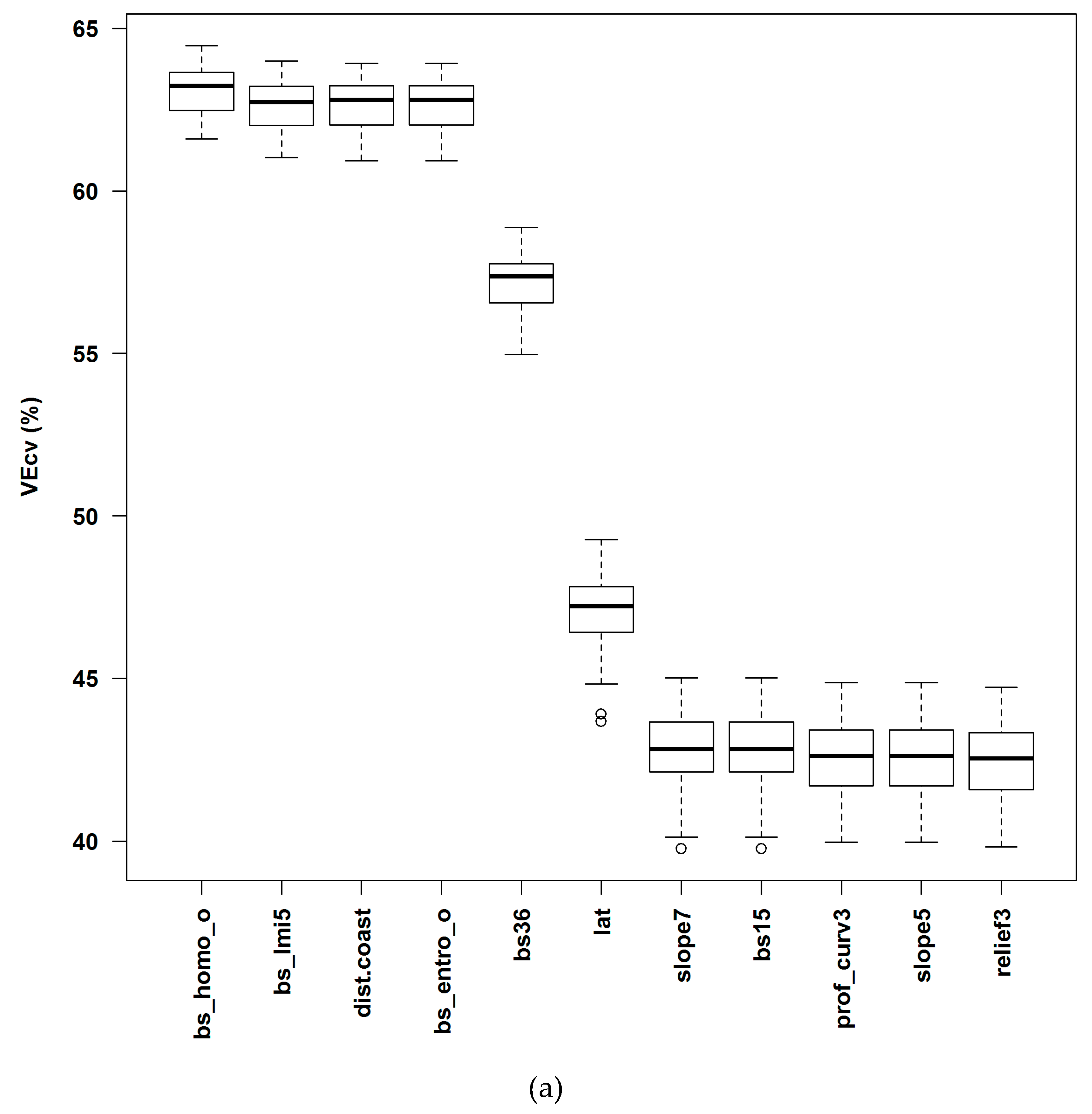
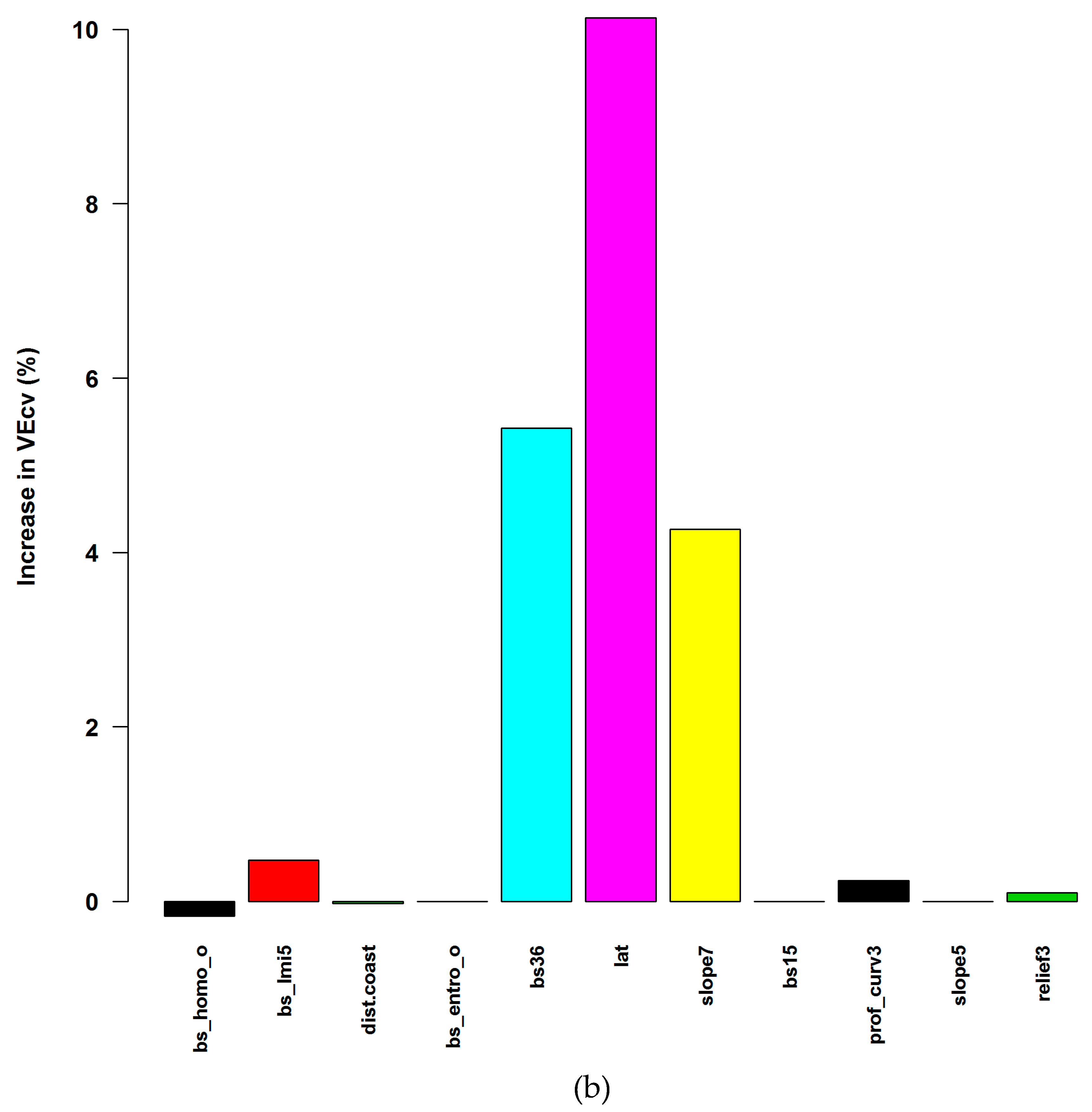
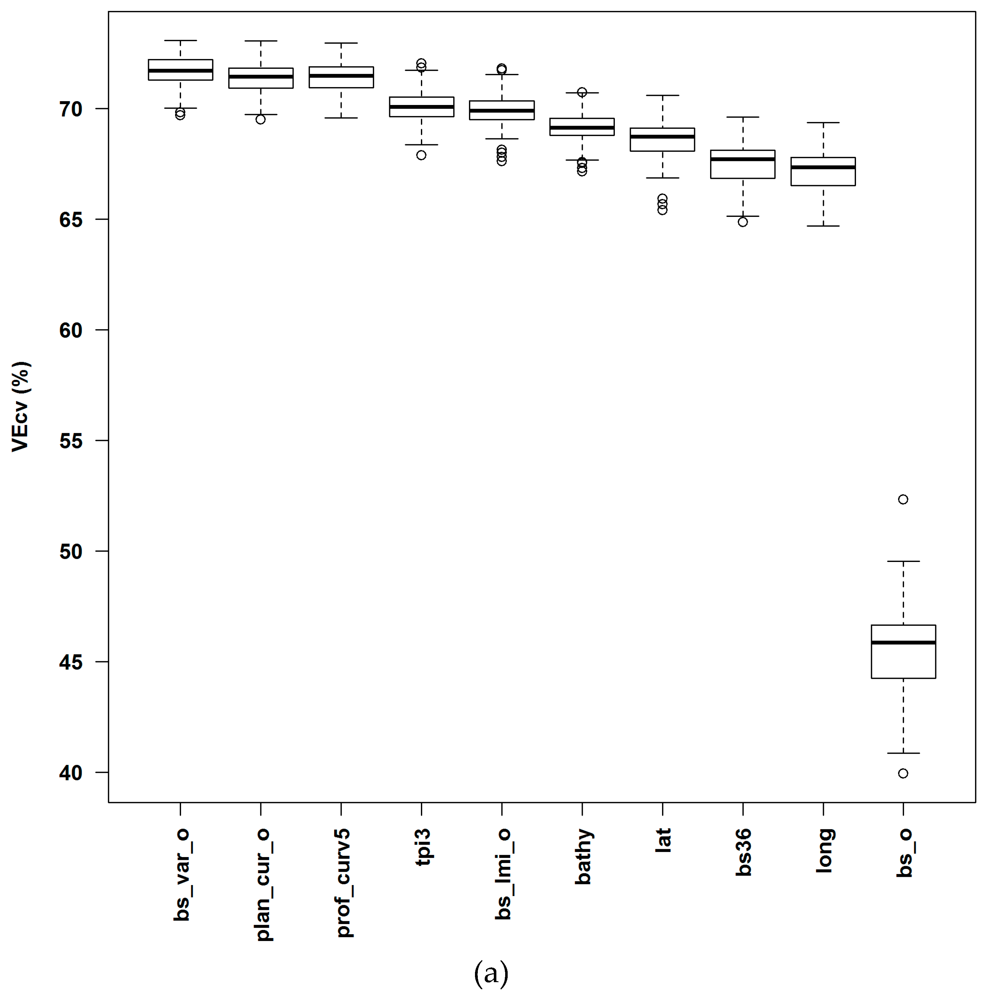
3.1.1. Averaged Variable Importance (AVI)

The predictive accuracy (VEcv) of RF gradually increased from model 1 (i.e., the model corresponding to plan_curv5) to model 34 (i.e., the model corresponding to bs23) in Figure 2a and reached a maximum VEcv for model 34. Sixteen important predictors were identified based on AVI (Table 5). The accuracy contributions of these variables varied from the most to the least in the following order: dist.coast, bs_o, lat, prof_curv5, bs36, bathy, bs_var_o, tpi3, long, bs_lmi_o, tpi_o, bs_entro7, bs25, bs15, bs_var5, and bs_entro5. However, the accuracy contributions of tpi_o, bs_entro7, bs25, bs15, bs_var5, and bs_entro5 were negative (Figure 2b).

3.1.2. Knowledge-Informed AVI (KIAVI2)

The final RF model selected using KIAVI2 for sand content contained 11 predictive variables (Figure 3, Table 5). The accuracy contributions of these variables ranked in the following order: dist.coast > bs_o > tpi3 > bs36 > bathy > lat > long > plan_curv_o > bs_lmi_o > bs_var_o > prof_curv5 (Figure 3b). Of these, one variable (i.e., prof_curv5) had a negligible negative accuracy contribution. However, its exclusion using KIAVI2 would result in a model with less predictive accuracy, so no further variable selection was conducted.
Rank order of AVI derived from RF changed with input predictors. For example, tpi3 was less important than prof_curv5 when all variables were included in the model (Figure 2a), but was more important than prof_curv5 in the final model (Figure 3a); and bs_var_o was more important than prof_curv-o when all variables were included in the model (Figure 2b), but was less important than prof_curv-o in the final model (Figure 3b).
Similarly, the initial input variables affected the accuracy contribution of predictive variables. For example, the accuracy contribution of prof_curv5 was positive when all variables were included in the model (Figure 2b), but was negative in the final model (Figure 3b).
Rank order of AVI of a variable and its accuracy contribution was not necessarily matched. For example, long was the third most important variable and tpi3 was the eighth in terms of AVI (Figure 2b), but the accuracy contribution of tpi was higher than that of long.

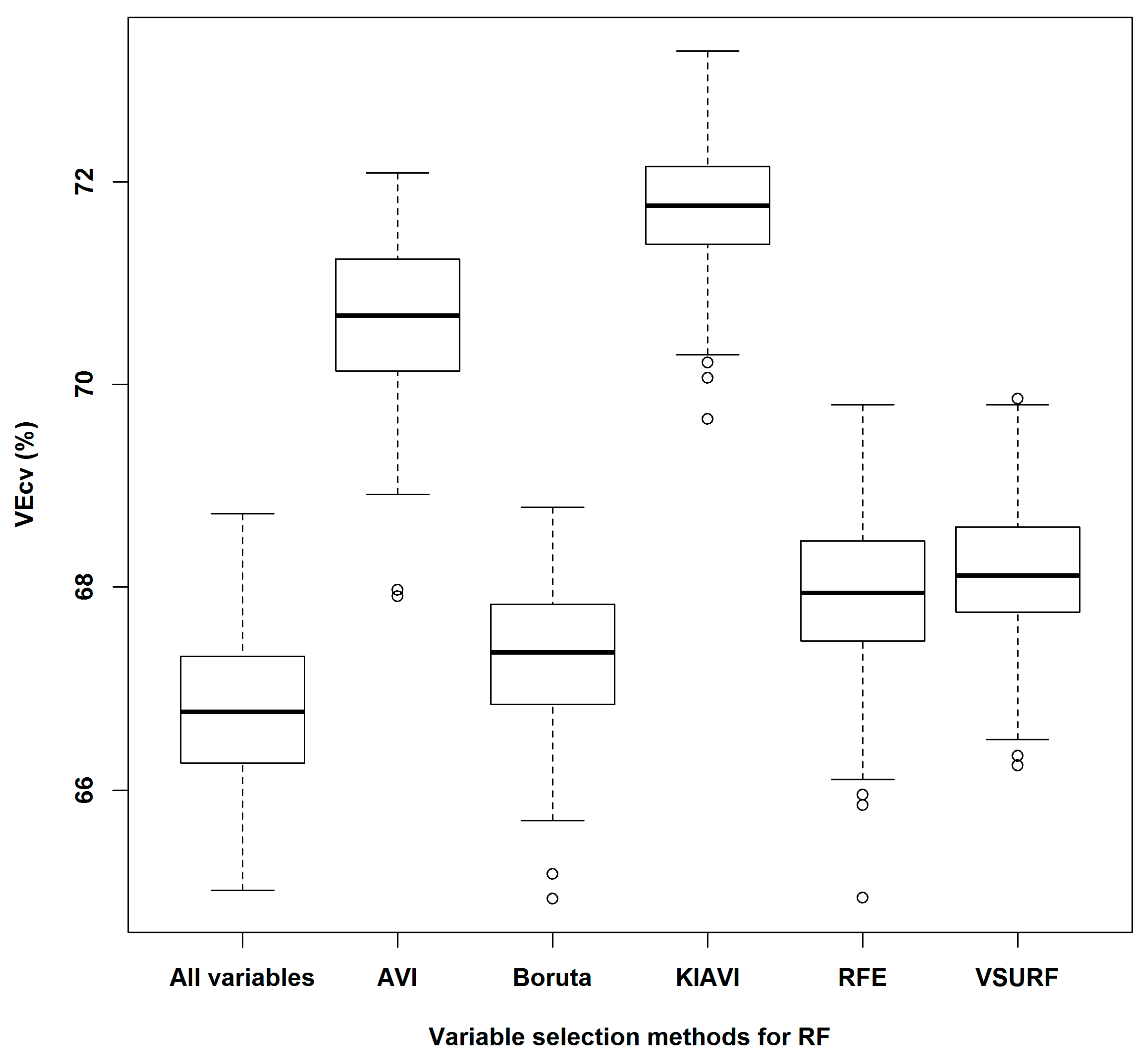
3.1.3. Boruta, Recursive Feature Selection (RFE), and Variable Selection Using RF (VSURF) and their Comparisons with AVI and KIAVI2

Three models were developed for RF based on the variable selection approach of Boruta, RFE, and VSURF. Thirty-one, four, and eleven variables were selected by using Boruta, RFE, and VSURF, respectively (Table 5). The variables selected using various methods were different, with only two variables (i.e., dist.coast and bs_o) selected by all five methods (Table 5). These two variables alone explained 67.19% variance in terms of VEcv (i.e., 45.55% by dist.coast and 21.64% by bs_o) (Figure 3a).
The accuracy of the predictive models developed for RF using various variable selection methods was compared in Figure 4 and Table 6. Among these variable selection methods, in terms of the accuracy of the predictive models identified, KIAVI2 was the best, followed by AVI, VSURF, RFE, Boruta, and the full model. The models developed by KIAVI2 were significantly more accurate than the models by other methods based on the Mann–Whitney tests (with p values < 0.0001), and the differences in terms of predictive accuracy were significant among all variable selection methods, with the exception of the difference between RFE and VSURF that was not significant (with a p value = 0.0959).

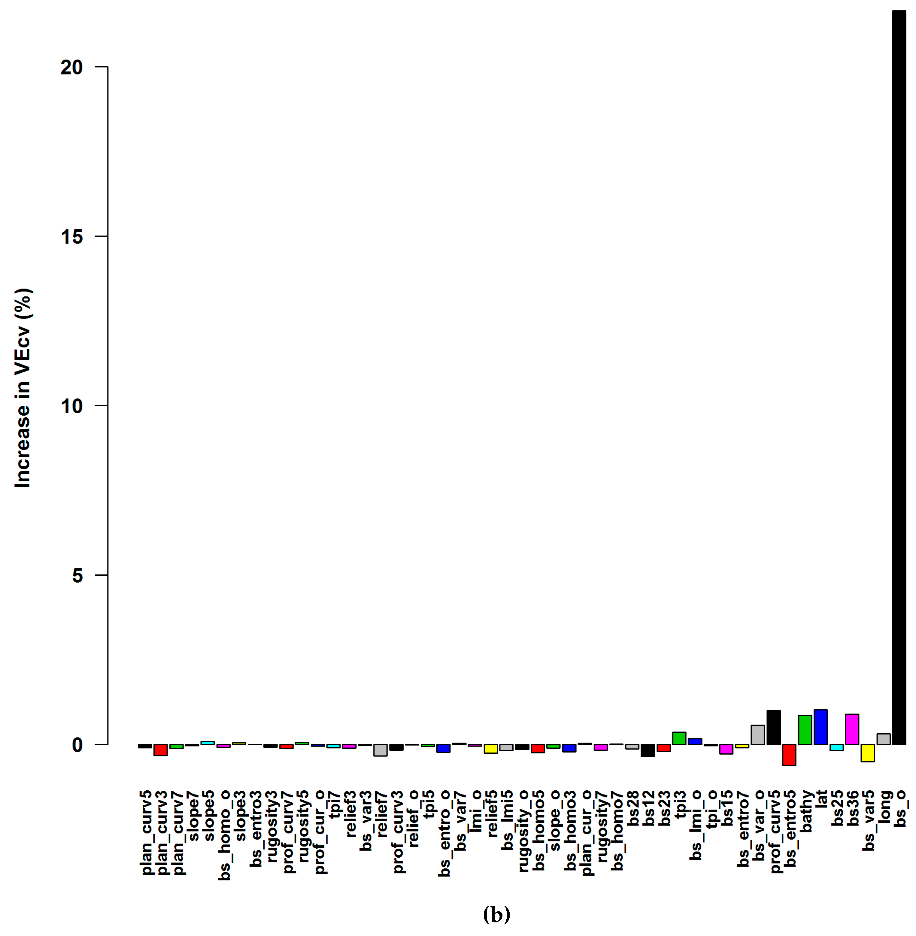
3.2. Variable Selection Methods for GBM

The final GBM model selected using KIRVI contained 13 predictive variables (Table 5, Figure 5). The accuracy contributions of these variables varied from the most to the least in the following order: relief7, prof_curv5, lat, bs36, slope7, bs_lmi5, prof_curv3, relief3, bs15, bs_entro_o, slope5, dist.coast, and bs_homo_o. Of these, the two most important variables (i.e., relief7 and prof_curv5) contributed 42.46% to the accuracy (Figure 5a), two variables (i.e., bs_homo_o and dist.coast) contributed negatively to the accuracy, and three variables (i.e., bs15, bs_entro_o, and slope5) had zero accuracy contribution. The rank order of RVI of a variable (Figure 5a) and the rank order of its accuracy contribution (Figure 5b) were not matched. However, the exclusion of these five variables using KIRVI resulted in a model with less predictive accuracy. The accuracy of the predictive models developed for GBM was compared in Table 7. The models developed by KIRVI were not significantly more accurate than the model using all available predictive variables based on the Mann–Whitney tests (with a p value = 0.1199).

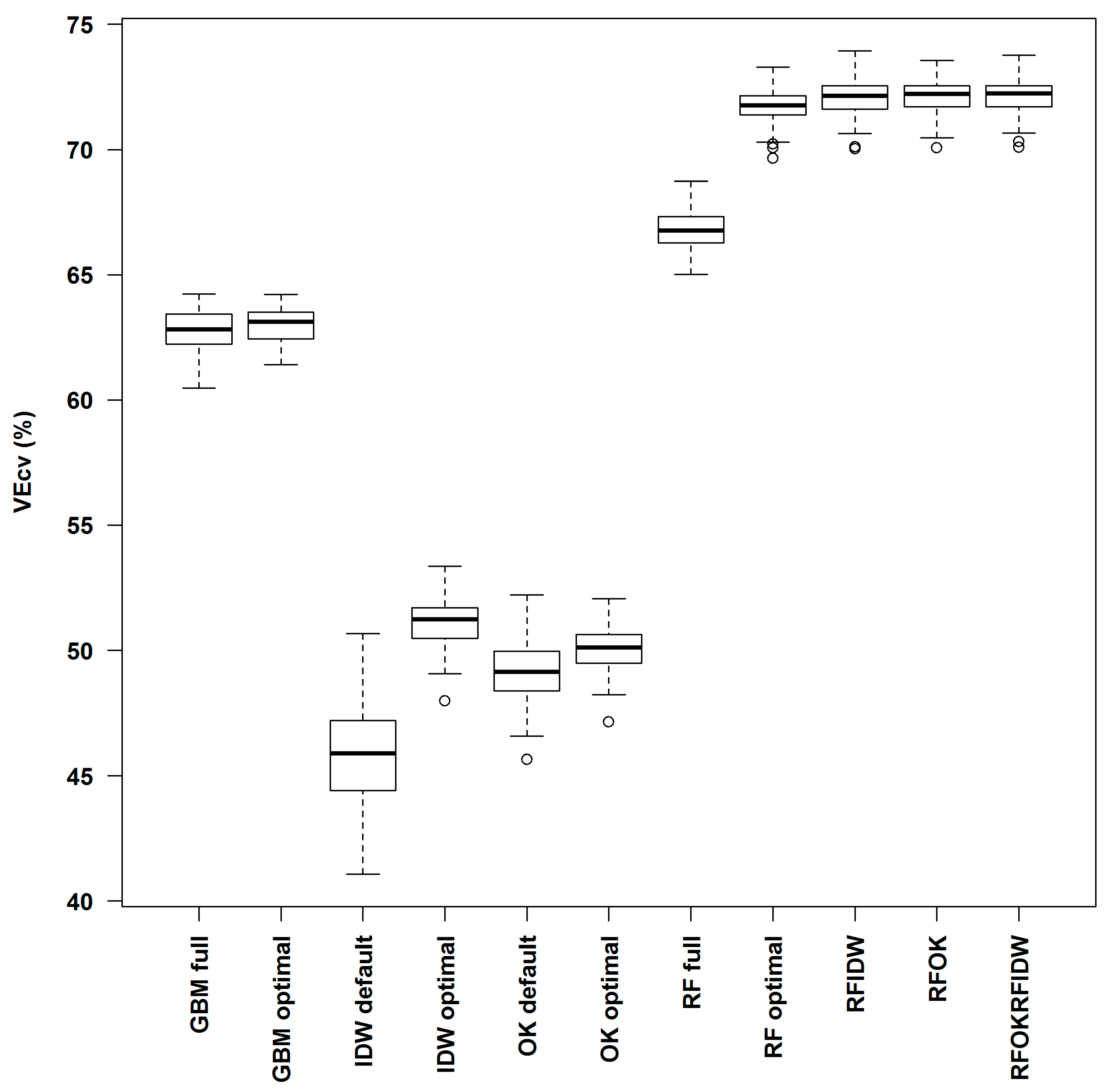
3.3. Comparison of Predictive Methods in Spm

The accuracy of predictive models developed for IDW, OK, GBM, RF, RFIDW, RFOK, and RFOKRFIDW is summarized in Figure 6 and compared in Table 7. The models developed for RFOK, RFIDW, and RFOKRFIDW were significantly more accurate than the models for all other methods based on the Mann–Whitney tests (with p values < 0.001). Among the models for RFOK, RFIDW, and RFOKRFIDW, the differences were not significant in terms of the Mann–Whitney tests. RFOKRFIDW had slightly increased the accuracy, although such improvement was marginal in comparison with RFOK and RFIDW in terms of the Mann–Whitney tests (with p values = 0.9795 and 0.6294). As a result, the predictive model developed using RFOKRFIDW was the most accurate model.

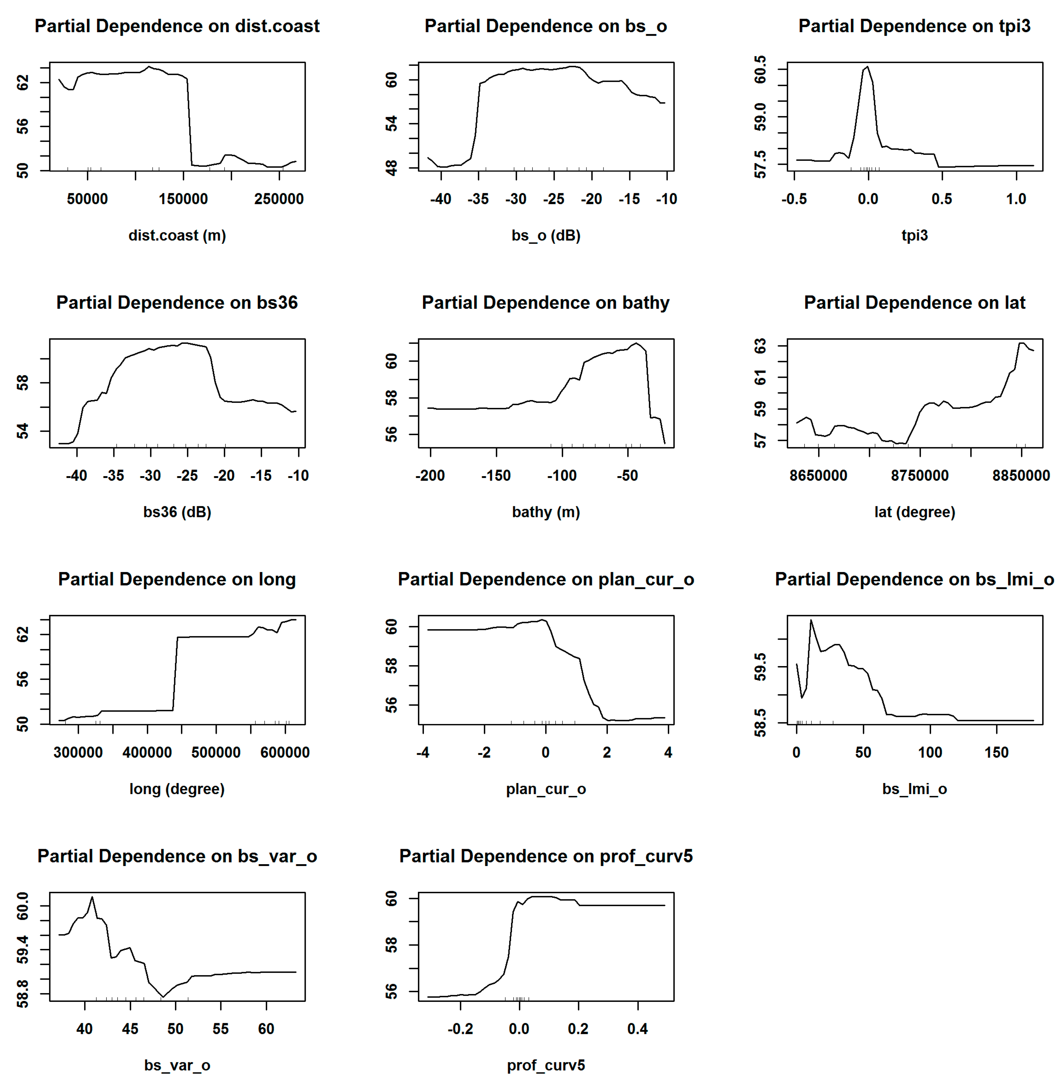
3.4. Predictions of Seabed Sand Content

Predictions of seabed sand content were generated using the most accurate predictive model based on RFOKRFIDW. The relationships of sand content with the selected predictors were non-linear (Figure 7). For example, sand content was relatively high and stable when dist.coast was less than 150 km, and then it sharply declined and remained low when dist.coast exceeded 150 km; an opposite pattern was observed for bs_o at −35 dB.
Sand content predictions are illustrated in Figure 8 for a portion of Area A. This area was chosen as an example because it contained highly contrasting geomorphic features and predictions. The predicted sand content was found to be relatively low on banks and deep valleys but high on the terraces and ridges.

4. Discussion

4.1. Bathymetry-Related Variables vs Backscatter-Related Variables for Predictions of Seabed Sand Content

Among the 11 predictive variables used in the final predictive model for sand content, dist.coast was the most important predictor in terms of its accuracy contribution. Although the underpinning mechanism is unknown and it is likely to be a proxy for water depth, dist.coast has been found to be a useful predictor for seabed sediments in Australia at national and regional scales [8,10,37,58] as well as for biodiversity at national and local scales [29,59].
Bathymetry, backscatter, and their derived variables all contributed to the predictive model. Bathymetry-related variables were bathy, tpi3, plan_curv_o, and prof_curv5, and backscatter-related variables were bs_o, bs36, bs_lmi_o, and bs_var_o) (Figure 3b). Backscatter-related variables contributed more than bathymetry-related variables to the predictive accuracy, and bs_o was identified as the second most important IVPA (Figure 3). In previous studies, backscatter and its derived variables were not used for seabed sediment predictions at national and regional scales because of their unavailability [7,8,10]. This study demonstrated the importance of backscatter-related variables to sediment predictive modelling. A similar finding was also evident in a previous study for predicting sponge species richness in this study region [29]. The importance of backscatter-related variables to sediment predictive modelling at local scales has been documented for other regions [4,14,60,61]. The importance of backscatter-related variables to predicting other environmental variables has also been documented previously in this study area [29,35]. All these findings highlight the importance of backscatter-related variables for improving the quality of sediment predictions.

4.2. Highly Correlated Predictive Variables

The inclusion of highly correlated predictors can improve predictive accuracy for RF (i.e., ρ = 0.96 for bs_o and bs36) (Figure 3b) and for GBM (i.e., ρ = 0.96 for slope5 and slope7) (Figure 5b). This is consistent with previous findings in other studies [8,29,35,36,42]. As discussed previously, correlated variables may be able to compensate for the small number of predictors as well as for the unavailability or unknown of causal variables in environmental sciences [29]. This finding further supports the recommendation that highly correlated variables should not be excluded in the preselecting predictors using correlation methods for machine learning methods such as RF and GBM [29]. The usefulness and selection of highly correlated variables should be determined by using variable selection methods, as discussed in Section 4.5.

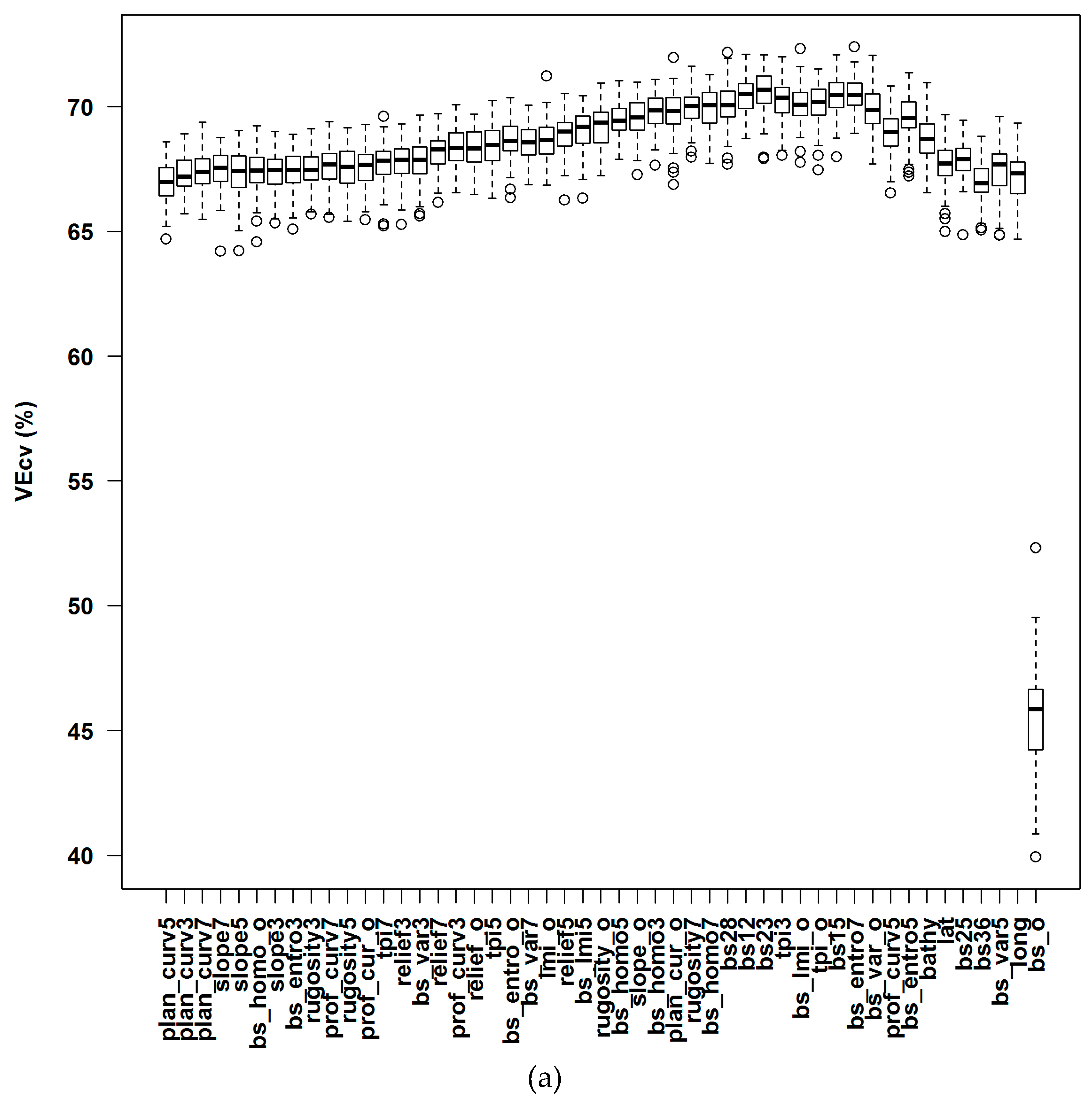
4.3. Variable Importance and Initial Input Predictive Variables for RF

Rank order of AVI derived from RF changes with input predictors in the model for RF in this study, which is consistent with previous findings [10,29,35]. This change suggests that if the least important variable is removed from the model, the relative importance of the remaining variables may change. This may explain why the model developed by using methods like RFE is less accurate than the model by AVI and KIAVI2 (Figure 4, Table 6). This is because in RFE the variable importance of all predictive variables was based on only the full model, and then subsequent variable removal was based on this information, but it failed to consider the above observed fact that the variable importance derived from RF may change with input predictors in the model. The dependence of AVI on the existing variables in the model may alter the order of the variable’s AVI, thus resulting in the exclusion of some variables that may be more important than the remaining ones in terms of their accuracy contribution, as discussed below.

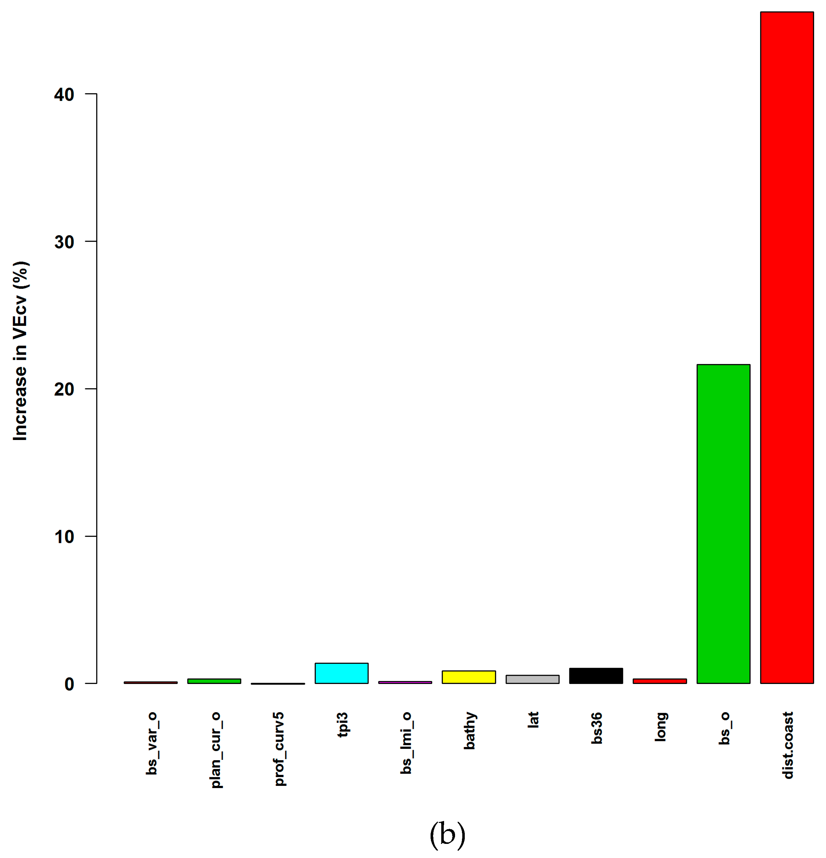
4.4. Accuracy Contribution and Initial Input Predictive Variables for RF

The rank order of accuracy contribution changed with the input predictors for RF in this study. This finding suggests that the status of IVPA changes with the initial input predictors, and unimportant variables can be identified as important variables if certain unimportant variables exist. This indicates that the accuracy contribution of a variable depends on the variable(s) already included in the model. This phenomenon was also found in previous studies [10,29,35]. It was also found that the inclusion of noisy or irrelevant predictors may reduce the possibility of the selection of important variables at each node split for each individual tree and, thus, reduce the predictive accuracy [9,37]. This suggests that preselection of predictors is important for predictive modelling using RF. However, this presents a challenge for preselection because in environmental sciences, the causal predictive variables are often unknown or unavailable, and proxy variables are used instead [29]. Apparently, this is an area worth further investigation in the future.

4.5. Variable Selection Methods for RF

Among several variable selection methods compared for RF in this study, the application of KIAVI2 leads to the most accurate predictive model for sand content. Thus, KIAVI2 is recommended for the future studies. It should be noted that in the process of variable selection, this method removes the variable with the lowest AVI by assuming that a variable with the lowest AVI also has the least accuracy contribution. However, in this study, the rank order of AVI of a variable and its accuracy contribution was found to be unmatched for RF, thus, the assumption does not hold true. This can cause difficulty for selecting predictive variables using KIAVI and KIAVI2 because a variable could be removed, due to its least AVI, despite its accuracy contribution may not be the least, even though the AVI was calculated for each newly formed dataset after removing the variable with the least AVI (see Table 4). This presents a challenge for variable selection for RF, although KIAVI2 was demonstrated to be the most accurate variable selection method in this study. It has been suggested that repeating the selection procedure based on IVPA and UVPA by using KIAVI may help to resolve this issue [29]. However, no further effort was taken to test and confirm this, so we recommend future studies test this or develop more reliable variable selection methods for RF, which is particularly important when the number of predictive variables is large [29,35].

4.6. Issues with Model Valuation and Selection Criteria for GBM

The rank order of RVI of a variable and the rank order of its accuracy contribution are not necessarily matched for GBM. This suggests that RVI of a variable is not consistent with its accuracy contribution. A similar phenomenon was also observed for RF in terms of AVI and accuracy contribution, as discussed in 4.3. The relevant discussion about the implications of such phenomenon for RF is also relevant for GBM. Although GBM is outperformed by RF in this study, it was found that GBM was more accurate than RF previously [32]. This may suggest that the performance of these methods is data-dependent.
The improvement to predictive accuracy by applying KIRVI to GBM model is minimal. This may suggest that for GBM modelling, variable selection may be either redundant or essential, but the improvement in accuracy is data-dependent. However, previous studies suggest that accuracy improvement is data-dependent because a GBM model based on a selected set of predictors [62] is more accurate than a GBM model based on a full dataset [29]. Hence, variable selection methods for GBM are necessary for identifying an optimal predictive model, and they need to be developed in the future. Variable selection methods for RF may provide a useful reference point for such development.

4.7. Predictive Accuracy of Seabed Sand Content

The hybrid methods applied in this study significantly improved predictive accuracy in comparison with other methods including RF and GBM (Table 7). This is consistent with previous findings in other studies [29,30,36,58]. The hybrid methods of machine learning with geostatistical methods were developed and have been applied to marine sediment data since 2008 with proven high predictive accuracy [7,8,9,37], but their applications to other data types or terrestrial data are still rare [30,32,33,63,64]. GBM was outperformed by RF in this study, but it performed similarly to RF for the sponge dataset in spm [62]. RFOKRFIDW only marginally improved the accuracy in comparison with the hybrid methods (i.e., RFOK and RFIDW). The possible reasons for such marginal effects by model averaging have been discussed previously [10]. These hybrid methods and their averaging are recommended for predicting environmental variables in the future.
The prediction accuracy (VEcv) of the most accurate model for RFOKRFIDW is 72.16%, which is higher than the average accuracy of predictive models published in environmental sciences [8,29,54]. The high performance of the hybrid methods can be attributed to features of RF and the ability to deal with both global trends, either spatially and/or environmentally, and local variations [10,29,37,58] as well as the use of backscatter-related predictive variables, despite the fact that the predictors used in this study are proxies instead of causal variables. This may further demonstrate the capability of the hybrid methods and highlights the importance of backscatter-related predictive variables, as discussed in 4.1.

4.8. Predictions of Seabed Sand Content and their Application

Predictions of seabed sand content were generally high (>50%) across study area A (Figure 8a). The contribution of the most important variable in the model (‘distance to coast’) to this result is accounted for by the location of area A within 140 km from the coast, with the RF model predicting that sand content is relatively high when the distance to coast was less than 150 km (Figure 7). However, the influence of this variable was largely unnoticeable spatially within area A, as it only covered a short range of dist.coast (i.e., 103–140 km), and other variables clearly played a more significant (and logical) role in the model (Figure 7 and Figure 8).
Highest sand content was mostly predicted on the terraces and ridges and was mainly due to the intermediate values of backscatter-derived variables bs_o and bs36 (ranging from −35 to −20 dB) (Figure 7 and Figure 8d). In contrast, the relatively low predicted sand content in deep valleys (Figure 1bA and Figure 8a) was mainly due to their associated low backscatter values (<−35 dB). Predicted sand content for shallower banks was also low but associated with higher backscatter values ((approximately 15 dB). This pattern is consistent with this area comprising a complex terrain of carbonate banks and shoals where sand is locally-sourced biogenic material from a range of producers (bivalves, gastropods, calcareous algae, and hard corals) [65] (Figure 7). For the shallow banks of area A, gravel content is known to be high [15,16], which accounts for the lower predicted sand content. The patterns of the predictions may also reflect the local variations associated with the remaining predictors, but their influences were barely noticeable. The non-linear relationships of sand content with the predictors were expected, as they have been also observed in previous studies for other environmental variables in this study area [29].
Although the major patterns were largely captured in the previously released sand predictions at 250 m [12] and 1000 m resolutions [11] (Figure 8b,c), more detailed patterns were revealed by these new predictions at 10 m resolution (Figure 8a). For example, sand content was previously predicted as low for the scarp feature along the flanks of the valley in area A, in comparison to the new model that utilized backscatter data. This suggests that the availability of backscatter-derived data for this study enables the model to generate more accurate predictions of sand content across diverse and complex seabed topography.
These findings provide important baseline information for the management and monitoring of seabed environments in the Timor Sea region, northern Australia. A key application of modelling sediment texture at such high spatial resolution lies in the association with potential seabed habitats, whereby sediment type is considered a surrogate for benthic biodiversity [5]. Thus, in predicting the likely distribution of broad sediment classes and linking this to seabed geomorphology provides greater insight into the potential occurrence of habitats. Examples include soft sediment (infaunal) biota that may concentrate in fine-grained (mud) sediment areas of marine plains and valleys, sessile biota (e.g., sponges) that might colonize coarse (gravel) sediment deposits on shallower banks and terraces, and areas of active sand bedforms where benthic communities may be sparse to absent. On this basis, these fine spatial-scale sediment predictions can support the design of monitoring programs that need to focus on specific biodiversity values of a given area, and they can contribute to more strategic management of Australia’s marine estate.

5. Conclusions

This is the first combined application of RF, its hybrid methods with OK and IDW, and GBM to seabed sediment predictions integrating bathymetry- and backscatter-derived data at fine resolution and a local scale. Backscatter-derived variables proved to be more important than bathymetry-derived variables for the modelling. The inclusion of highly correlated predictors can improve predictive accuracy. KIAVI2 is recommended for future RF modelling. The rank order of AVI of a variable and the rank order of its accuracy contribution are not necessarily matched for RF, which can cause difficulty for selecting predictive variables using KIAVI and KIAVI2 and presents a challenge for variable selection for RF that is worthy of further investigation. Furthermore, variable importance and accuracy contribution are dependent on the initial set of input predictors. Variable selection methods for GBM need to be developed in the future, and variable selection methods for RF may provide useful references for such development. The hybrid methods of RF, geostatistics, and their averaging can significantly improve predictive accuracy in comparison to other methods, including RF and GBM, and are recommended for predicting environmental variables in the future. Moreover, the non-linear relationships revealed and improved sand content predictions provide important baseline information for the management and monitoring of priority marine environments.

Supplementary Materials

The following are available online at https://www.mdpi.com/2076-3263/9/4/180/s1: Sediments_samples_predictors_timor_sea.csv. https://www.mdpi.com/2076-3263/9/4/180/s2: Acquisition and processing of multibeam bathymetry, backscatter and their derived variables.

Author Contributions

Conceptualization, J.L. and S.N.; methodology, J.L., J.S., and Z.H.; software, J.L.; validation, J.L.; formal analysis, J.L.; data curation, J.S., Z.H., S.N., and J.L.; writing—original draft preparation, J.L.; writing—review and editing, S.N., J.S., and J.L.; visualization, J.L., J.S.

Acknowledgments

Datasets used in this study were collected as part of the Australian Government’s Offshore Energy Security Program (2007–2011) and the National Environmental Research Program Marine Biodiversity Hub (2011–2015). We thank Andrew Carroll and Neil Symington at Geoscience Australia for their valuable comments and suggestions on an earlier draft. This paper is published with the permission of the Chief Executive Officer, Geoscience Australia.

Conflicts of Interest

The authors declare no conflict of interest.

References

  1. Verfaillie, E.; Van Lancker, V.; Van Meirvenne, M. Multivariate geostatistics for the predictive modelling of the surficial sand distribution in shelf seas. Cont. Shelf Res. 2006, 26, 2454–2468. [Google Scholar] [CrossRef]
  2. Verfaillie, E.; Du Four, I.; Van Meirvenne, M.; Van Lancker, V. Geostatistical modeling of sedimentological parameters using multi-scale terrain variables: Application along the Belgian Part of the North Sea. Int. J. Geogr. Inf. Sci. 2008. [Google Scholar] [CrossRef]
  3. Stephens, D.; Diesing, M. Towards quantitative spatial models of seabed sediment composition. PLoS ONE 2015, 10, e0142502. [Google Scholar] [CrossRef] [PubMed]
  4. Huang, Z.; Nichol, S.; Siwabessy, P.J.W.; Daniell, J.; Brooke, B.P. Predictive Modelling of Seabed Sediment Parameters Using Multibeam Acoustic Data: A Case Study on the Carnarvon Shelf, Western Australia. Int. J. Geogr. Inf. Sci. 2012, 26, 283–307. [Google Scholar] [CrossRef]
  5. McArthur, M.A.; Brooke, B.P.; Przeslawski, R.; Ryan, D.A.; Lucieer, V.L.; Nichol, S.; McCallum, A.W.; Mellin, C.; Cresswell, I.D.; Radke, L.C. On the use of abiotic surrogates to describe marine benthic biodiversity. Estuar. Coast. Shelf Sci. 2010, 88, 21–32. [Google Scholar] [CrossRef]
  6. Przeslawski, R.; Daniell, J.; Anderson, T.; Vaughn Barrie, J.; Heap, A.; Hughes, M.; Li, J.; Potter, A.; Radke, L.; Siwabessy, J.; et al. Seabed Habitats and Hazards of the Joseph Bonaparte Gulf and Timor Sea, Northern Australia; Geoscience Australia, Record 2008/23; Geoscience Australia: Canberra, ACT, Australia, 2011; 69p.
  7. Li, J.; Potter, A.; Huang, Z.; Daniell, J.J.; Heap, A. Predicting Seabed Mud Content across the Australian Margin: Comparison of Statistical and Mathematical Techniques Using a Simulation Experiment; Geoscience Australia, Record 2010/11; Geoscience Australia: Canberra, ACT, Australia, 2010; 146p.
  8. Li, J.; Potter, A.; Huang, Z.; Heap, A. Predicting Seabed Sand Content across the Australian Margin Using Machine Learning and Geostatistical Methods; Geoscience Australia, Record 2012/48; Geoscience Australia: Canberra, ACT, Australia, 2012; 115p.
  9. Li, J.; Heap, A.; Potter, A.; Daniell, J.J. Predicting Seabed Mud Content across the Australian Margin II: Performance of Machine Learning Methods and Their Combination with Ordinary Kriging and Inverse Distance Squared; Geoscience Australia, Record 2011/07; Geoscience Australia: Canberra, ACT, Australia, 2011; 69p.
  10. Li, J. Predicting the spatial distribution of seabed gravel content using random forest, spatial interpolation methods and their hybrid methods. In Proceedings of the International Congress on Modelling and Simulation (MODSIM) 2013, Adelaide, Australia, 1–6 December 2013; pp. 394–400. [Google Scholar]
  11. Li, J.; Heap, A.; Potter, A.; Huang, Z. Seabed sand content across the Australian continental EEZ 2011. GEOCAT: 71982. Data format: Digital ArcGIS-grid (ArcInfo grid) in 0.01 decimal degree resolution in WGS84 and digital ASCII text in 0.01 decimal degree resolution in WGS84. 2011. Available online: http://pid.geoscience.gov.au/dataset/ga/71982 (accessed on 17 April 2019).
  12. Li, J. Predicted seabed sand content in the north-northwest region of the Australian continental EEZ 2013. GEOCAT: 76999. Data format: Digital ArcGIS-grid (ArcInfo grid) in 0.0025 decimal degree resolution in WGS84. 2013. Available online: http://pid.geoscience.gov.au/dataset/ga/76999 (accessed on 17 April 2019).
  13. Diesing, M.; Mitchell, P.; Stephens, D. Image-based seabed classification: What can we learn from terrestrial remote sensing? ICES J. Mar. Sci. 2016, fsw 118. [Google Scholar] [CrossRef]
  14. Lark, R.M.; Marchant, B.P.; Dove, D.; Green, S.L.; Stewart, H.; Diesing, M. Combining observations with acoustic swath bathymetry and backscatter to map seabed sediment texture classes: The empirical best linear unbiased predi. Sediment. Geol. 2015, 328, 17–32. [Google Scholar] [CrossRef]
  15. Heap, A.D.; Przeslawski, R.; Radke, L.; Trafford, J.; Battershill, C.; Party, S. Seabed Environments of the Eastern Joseph Bonaparte Gulf, Northern Australia. Sol4934—Post-survey Report; Geoscience Australia, Record 2010/09; Geoscience Australia: Canberra, ACT, Australia, 2010; 78p.
  16. Anderson, T.J.; Nichol, S.; Radke, L.; Heap, A.D.; Battershill, C.; Hughes, M.; Siwabessy, P.J.; Barrie, V.; Alvarez de Glasby, B.; Tran, M.; et al. Seabed Environments of the Eastern Joseph Bonaparte Gulf, Northern Australia: GA0325/Sol5117—Post-Survey Report; Geoscience Australia, Record 2011/08; Geoscience Australia: Canberra, ACT, Australia, 2011; 59p.
  17. Nichol, S.; Howard, F.; Kool, J.; Stowar, M.; Bouchet, P.; Radke, L.; Siwabessy, J.; Przeslawski, R.; Picard, K.; Alvarez de Glasby, B.; et al. Oceanic Shoals Commonwealth Marine Reserve (Timor Sea) Biodiveristy Survey: GA0339/SOL5650 Post-Survey Report; Geoscience Australia, Record 2013/38; Geoscience Australia: Canberra, ACT, Australia, 2013.
  18. Li, J.; Heap, A.D. Spatial interpolation methods applied in the environmental sciences: A review. Environ. Model. Softw. 2014, 53, 173–189. [Google Scholar] [CrossRef]
  19. Li, J.; Heap, A. A Review of Spatial Interpolation Methods for Environmental Scientists; Geoscience Australia, Record 2008/23; Geoscience Australia: Canberra, ACT, Australia, 2008; 137p.
  20. Li, J.; Heap, A. A review of comparative studies of spatial interpolation methods in environmental sciences: Performance and impact factors. Ecol. Inform. 2011, 6, 228–241. [Google Scholar] [CrossRef]
  21. Li, J. Predicted seabed gravel content in the north-northwest region of the Australian continental EEZ 2013. GEOCAT: 76997. Data format: Digital ArcGIS-grid (ArcInfo grid) in 0.0025 decimal degree resolution in WGS84. 2013. Available online: http://pid.geoscience.gov.au/dataset/ga/76997 (accessed on 17 April 2019).
  22. Cutler, D.R.; Edwards, T.C.J.; Beard, K.H.; Cutler, A.; Hess, K.T.; Gibson, J.; Lawler, J.J. Random forests for classification in ecology. Ecography 2007, 88, 2783–2792. [Google Scholar] [CrossRef]
  23. Diaz-Uriarte, R.; de Andres, S.A. Gene selection and classification of microarray data using random forest. BMC Bioinform. 2006, 7, 1–13. [Google Scholar] [CrossRef] [PubMed]
  24. Shan, Y.; Paull, D.; McKay, R.I. Machine learning of poorly predictable ecological data. Ecol. Model. 2006, 195, 129–138. [Google Scholar] [CrossRef]
  25. Prasad, A.M.; Iverson, L.R.; Liaw, A. Newer classification and regression tree techniques: Bagging and random forests for ecological prediction. Ecosystems 2006, 9, 181–199. [Google Scholar] [CrossRef]
  26. Drake, J.M.; Randin, C.; Guisan, A. Modelling ecological niches with support vector machines. J. Appl. Ecol. 2006, 43, 424–432. [Google Scholar] [CrossRef]
  27. Elith, J.; Leathwick, J.R.; Hastie, T. A working guide to boosted regression trees. J. Anim. Ecol. 2008, 77, 802–813. [Google Scholar] [CrossRef] [PubMed]
  28. Marmion, M.; Parviainen, M.; Luoto, M.; Heikkinen, R.K.; Thuiller, W. Evaluation of consensus methods in predictive species distribution modelling. Divers. Distrib. 2009, 15, 59–69. [Google Scholar] [CrossRef]
  29. Li, J.; Alvarez, B.; Siwabessy, J.; Tran, M.; Huang, Z.; Przeslawski, R.; Radke, L.; Howard, F.; Nichol, S. Application of random forest, generalised linear model and their hybrid methods with geostatistical techniques to count data: Predicting sponge species richness. Environ. Model. Softw. 2017, 97, 112–129. [Google Scholar] [CrossRef]
  30. Sanabria, L.A.; Qin, X.; Li, J.; Cechet, R.P.; Lucas, C. Spatial interpolation of McArthur’s forest fire danger index across Australia: Observational study. Environ. Model. Softw. 2013, 50, 37–50. [Google Scholar] [CrossRef]
  31. Sanabria, L.A.; Cechet, R.P.; Li, J. Mapping of Australian Fire Weather Potential: Observational and modelling studies. In Proceedings of the 20th International Congress on Modelling and Simulation (MODSIM2013), Adelaide, Australia, 1–6 December 2013; pp. 242–248. [Google Scholar]
  32. Appelhans, T.; Mwangomo, E.; Hardy, D.R.; Hemp, A.; Nauss, T. Evaluating machine learning approaches for the interpolation of monthly air temperature at Mt. Kilimanjaro, Tanzania. Spat. Stat. 2015, 14, 91–113. [Google Scholar] [CrossRef]
  33. Tadić, J.M.; Ilić, V.; Biraud, S. Examination of geostatistical and machine-learning techniques as interpolaters in anisotropic atmospheric environments. Atmos. Environ. 2015, 111, 28–38. [Google Scholar] [CrossRef]
  34. Li, J. A new R package for spatial predictive modelling: spm. In Proceedings of the useR! 2018, Brisbane, Australia, 10–13 July 2018. [Google Scholar]
  35. Li, J.; Tran, M.; Siwabessy, J. Selecting optimal random forest predictive models: A case study on predicting the spatial distribution of seabed hardness. PLoS ONE 2016, 11, e0149089. [Google Scholar] [CrossRef]
  36. Li, J. Predictive Modelling Using Random Forest and Its Hybrid Methods with Geostatistical Techniques in Marine Environmental Geosciences. In Proceedings of the Eleventh Australasian Data Mining Conference (AusDM 2013), Canberra, Australia, 13–15 November 2013. [Google Scholar]
  37. Li, J.; Heap, A.D.; Potter, A.; Daniell, J. Application of machine learning methods to spatial interpolation of environmental variables. Environ. Model. Softw. 2011, 26, 1647–1659. [Google Scholar] [CrossRef]
  38. Li, J.; Potter, A.; Heap, A. Irrelevant Inputs and Parameter Choices: Do They Matter to Random Forest for Predicting Marine Environmental Variables? In Proceedings of the Australian Statistical Conference 2012, Adelaide, Australia, 9–12 July 2012. [Google Scholar]
  39. Kursa, M.B.; Rudnicki, W.R. Feature Selection with the Boruta Package. J. Stat. Softw. 2010, 36, 1–13. [Google Scholar] [CrossRef]
  40. Genuer, R.; Poggi, J.M.; Tuleau-Malot, C. VSURF: Variable Selection Using Random Forests, R Package Version 1.0.2; 2015. Available online: https://CRAN.R-project.org/package=VSURF (accessed on 17 April 2019).
  41. Li, J.; Alvarez, B.; Siwabessy, J.; Tran, M.; Huang, Z.; Przeslawski, R.; Radke, L.; Howard, F.; Nichol, S. Selecting predictors to form the most accurate predictive model for count data. In Proceedings of the International Congress on Modelling and Simulation (MODSIM) 2017, Hobart, Australia, 3–8 December 2017. [Google Scholar]
  42. Li, J.; Siwabessy, J.; Tran, M.; Huang, Z.; Heap, A. Predicting Seabed Hardness Using Random Forest in R. In Data Mining Applications with R; Zhao, Y., Cen, Y., Eds.; Elsevier: Amsterdam, The Netherlands, 2014; pp. 299–329. [Google Scholar]
  43. Radke, L.C.; Li, J.; Douglas, G.; Przeslawski, R.; Nichol, S.; Siwabessy, J.; Huang, Z.; Trafford, J.; Watson, T.; Whiteway, T. Characterising sediments for a tropical sediment-starved shelf using cluster analysis of physical and geochemical variables. Environ. Chem. 2015, 12, 204–226. [Google Scholar] [CrossRef]
  44. Radke, L.; Nicholas, T.; Thompson, P.; Li, J.; Raes, E.; Carey, M.; Atkinson, I.; Huang, Z.; Trafford, J.; Nichol, S. Baseline biogeochemical data from Australia’s continental margin links seabed sediments to water column characteristics. Mar. Freshw. Res. 2017. [Google Scholar] [CrossRef]
  45. De Moustier, C.P.; Alexandrou, D. Angular dependence of 12-kHz seafloor acoustic backscatter. J. Acoust. Soc. Am. 1991, 90, 522–531. [Google Scholar] [CrossRef]
  46. Siwabessy, P.J.W.; Gavrilov, A.N.; Duncan, A.N.; Parnum, I.M. Analysis of statistics of backscatter strength from different seafloor habitats. In Proceedings of the Conference of the Australasian Acoustical Societies, Acoustics 2006, Christchurch, New Zealand, 20–22 November 2006; pp. 507–514. [Google Scholar]
  47. Siwabessy, P.J.W.; Daniell, J.; Li, J.; Huang, Z.; Heap, A.D.; Nichol, S.; Anderson, T.J.; Tran, M. Methodologies for Seabed Substrate Characterisation Using Multibeam Bathymetry, Backscatter and Video Data: A Case Study from the Carbonate Banks of the Timor Sea, Northern Australia; Geoscience Australia, Record 2013/11; Geoscience Australia: Canberra, ACT, Australia, 2013; 82p.
  48. Liaw, A.; Wiener, M. Classification and regression by randomForest. R News 2002, 2, 18–22. [Google Scholar]
  49. Kuhn, M. caret: Classification and Regression Training. R package version 60-30. 2014. Available online: http://CRAN.R-project.org/package=caret (accessed on 17 April 2019).
  50. Li, J.; Alvarez, B.; Siwabessy, J.; Tran, M.; Huang, Z.; Przeslawski, R.; Radke, L.; Howard, F.; Nichol, S. Spatial distribution of sponge species richness: Lessons learned from spatial predictive modelling and pattern predictions. In Proceedings of the Australian Marine Sciences Association (AMSA) Conference, Adelaide, Australia, 1–5 July 2018. [Google Scholar]
  51. Smith, S.J.; Ellis, N.; Pitcher, C.R. Conditional variable importance in R package extendedForest. Available online: http://gradientforest.r-forge.r-project.org/Conditional-importance.pdf (accessed on 17 April 2019).
  52. Hastie, T.; Tibshirani, R.; Friedman, J. The Elements of Statistical Learning: Data Mining, Inference, and Prediction, 2nd ed.; Springer: New York, NY, USA, 2009; p. 763. [Google Scholar]
  53. Kohavi, R. A study of cross-validation and bootstrap for accuracy estimation and model selection. In Proceedings of the International Joint Conference on Artificial Intelligence (IJCAI), Montreal, QC, Canada, 20–25 August 1995; pp. 1137–1143. [Google Scholar]
  54. Li, J. Assessing spatial predictive models in the environmental sciences: Accuracy measures, data variation and variance explained. Environ. Model. Softw. 2016, 80, 1–8. [Google Scholar] [CrossRef]
  55. R Development Core Team. R: A Language and Environment for Statistical Computing; R Foundation for Statistical Computing: Vienna, Austria, 2015. [Google Scholar]
  56. Pebesma, E.J. Multivariable geostatistics in S: The gstat package. Comput. Geosci. 2004, 30, 683–691. [Google Scholar] [CrossRef]
  57. Ridgeway, G. gbm: Generalized Boosted Regression Models, R package version 2.1.3. 2017. Available online: https://CRAN.R-project.org/package=gbm (accessed on 17 April 2019).
  58. Li, J.; Heap, A.D.; Potter, A.; Huang, Z.; Daniell, J. Can we improve the spatial predictions of seabed sediments? A case study of spatial interpolation of mud content across the southwest Australian margin. Cont. Shelf Res. 2011, 31, 1365–1376. [Google Scholar] [CrossRef]
  59. Huang, Z.; Brooke, B.; Li, J. Performance of predictive models in marine benthic environments based on predictions of sponge distribution on the Australian continental shelf. Ecol. Inform. 2011, 6, 205–216. [Google Scholar] [CrossRef]
  60. Stephens, D.; Diesing, M. A Comparison of Supervised Classification Methods for the Prediction of Substrate Type Using Multibeam Acoustic and Legacy Grain-Size Data. PLoS ONE 2014, 9, e93950. [Google Scholar]
  61. Diesing, M.; Green, S.L.; Stephens, D.; Lark, R.M.; Stewart, H.A.; Dove, D. Mapping seabed sediments: Comparison of manual, geostatistical, object-based image analysis and machine learning approaches. Cont. Shelf Res. 2014, 84, 107–109. [Google Scholar] [CrossRef]
  62. Li, J. spm: Spatial Predictive Modelling, R package version 1.1.0. 2018. Available online: https://CRAN.R-project.org/package=spm (accessed on 17 April 2019).
  63. Hengl, T.; Heuvelink, G.B.M.; Kempen, B.; Leenaars, J.G.B.; Walsh, M.G.; Shepherd, K.D.; Sila, A.; MacMillan, R.A.; de Jesus, J.M.; Tamene, L.; et al. Mapping Soil Properties of Africa at 250 m Resolution: Random Forests Significantly Improve Current Predictions. PLoS ONE 2015, 10, e0125814. [Google Scholar] [CrossRef] [PubMed]
  64. Reinhardt, K.; Samimi, C. Comparison of different wind data interpolation methods for a region with complex terrain in Central Asia. Clim. Dyn. 2018, 51, 3635–3652. [Google Scholar] [CrossRef]
  65. Przeslawski, R.; Glasby, C.; Nichol, S. Polychaetes (Annelida) of the Oceanic Shoals region, northern Australia: Considering small macrofauna in marine management. Mar. Freshw. Res. 2019, 70, 307–321. [Google Scholar] [CrossRef]
Figure 1. (a) Location of the study areas (A–H) and associated geomorphic features in the Timor Sea region, northern Australian marine with bathymetry. Also showing the border of Oceanic Shoals Marine Park (grey line) and key ecological features (KEFs) of the region: the carbonate banks and terraces of the Van Diemen Rise (blue), the carbonate banks and terraces of the Sahul Shelf (yellow), and the pinnacles of the Bonaparte Basin (black). (b) Seabed sampling locations (black dots) within each study area overlaid with associated geomorphic features.
Geosciences 09 00180 g001aGeosciences 09 00180 g001b
Figure 2. (a) Accuracy of 49 predictive models with the incremental removal of each corresponding least important predictive variable for sand content based on the averages over 100 iterations of 10-fold cross-validations, with variable elimination based on their averaged variable importance (over 100 simulations, see the avi function in spm for details). The remaining variable in the last model (i.e., the model corresponding to bs_o) is dist.coast. (b) Contribution of each predictive variable to predictive accuracy of RF models. The contribution of dist.coast (i.e., 45.55%) can be obtained from Figure 2a as it is the only remaining predictor in the last model corresponding to bs_o.
Geosciences 09 00180 g002aGeosciences 09 00180 g002b
Figure 3. (a) Accuracy of predictive models with the removal of each least important predictive variable based on the averages over 100 iterations of 10-fold cross-validations for seabed sand content, with variable elimination based on their averaged variable importance (over 100 simulations) using KIAVI2. The remaining variable in the last model (i.e., the model corresponding to bs_o) is dist.coast. (b) Contribution of each predictive variable to predictive accuracy of the final RF model. The contribution of dist.coast (i.e., 45.55%) can be obtained from Figure 2a as it is the only remaining predictor in the last model.
Geosciences 09 00180 g003aGeosciences 09 00180 g003b
Figure 4. The VEcv (%) of the most accurate predictive models based on the averages over 100 iterations of 10-fold cross-validations for seabed sand content developed for RF using various variable selection methods.
Geosciences 09 00180 g004
Figure 5. (a) Accuracy of predictive models with the incremental removal of each least important predictive variable based on the averages over 100 iterations of 10-fold cross-validations for seabed sand content, with variable elimination based on their relative variable influence using KIRVI. The remaining variables in the last model (i.e., the model corresponding to relief3) are relief7 and prof_curv5. (b) Contribution of each predictive variable to predictive accuracy of the final GBM model, with an exception of relief7 and prof_curv5 (their combined accuracy contribution is 42.46%).
Geosciences 09 00180 g005aGeosciences 09 00180 g005b
Figure 6. The VEcv (%) of the predictive models for GBM, IDW, OK, RF, RFIDW, RFOK and RFOKRFIDW based on the averages over 100 iterations of 10-fold cross-validations for seabed sand content.
Geosciences 09 00180 g006
Figure 7. Partial plot of the most accurate RF model based on the order of their contributions in terms of VEcv, indicating the relationships of seabed sand content to the 11 predictive variables in the RF model.
Geosciences 09 00180 g007
Figure 8. Spatial distribution of seabed sand content and relevant predictive variables for a portion of area A in Timor Sea: (a) sand content at 10 m resolution (this study), (b) sand content at 250 m resolution from a previous study [12], (c) sand content at 1000 m resolution from a previous study [11], (d) bs_o (since bs36 showed a similar pattern as bs_o, it is not displayed here), (e) tpi3, (f) bathy, (g) plan_curv_o, (h) bs_lmi_o, (i) bs_var_o, and (j) prof_curv5.
Geosciences 09 00180 g008
Table 1. Predictive variables and their corresponding number for sand content.
No.Predictive VariableUnitNo.Predictive VariableUnit
1longdegree26slope7degree
2latdegree27rugosity3
3bs25dB28rugosity5
4bs_entro_o3 29rugosity7
5bs_entro_o5 30tpi3
6bs_entro_o7 31tpi5
7bs_homo3 32tpi7
8bs_homo5 33bs12
9bs_homo7 34bs15
10bs_var3 35bs23
11bs_var5 36bs28
12bs_var7 37bs36
13bs_lmi5 38dist.coastm
14bathym39bs_odB
15plan_curv3 40bs_homo_o
16plan_curv5 41bs_entro_o
17plan_curv7 42bs_var_o
18prof_curv3 43bs_lmi_o
19prof_curv5 44lmi_o
20prof_curv7 45tpi_o
21relief3m46slope_o
22relief5m47plan_cur_o
23relief7m48prof_cur_o
24slope3degree49relief_om
25slope5degree50rugosity_o
Table 2. Full name for the abbreviations of all modelling methods, feature selection methods, and measures of model performance in this study.
AbbreviationFull NameType
IDWInverse distance weighting Modelling methods
OKOrdinary kriging
GBMGeneralized boosted regression modelling
RFRandom forest
RFIDWThe hybrid of RF with IDW
RFOKThe hybrid of RF with OK
RFOKRFIDWThe average of RFOK and RFIDW
AVIAveraged variable importanceSelection methods
KIAVIKnowledge-informed AVI
RVIRelative variable influence
KIRVIKnowledge-informed RVI (KIRVI)
RFERecursive feature selection
VSURFVariable selection using RF
VEcvVariance explained by predictive models Accuracy measure
Table 3. Parameters used for each predictive model in relevant functions in spm.
Distance Power (idp)Window Size (nmax)Variogram Model (vgm.args)
IDW default212
IDW optimal0.619
OK default 12Sph
OK optimal 19Sph
RFIDW0.111
RFOK 17Lin
Table 4. A procedure for identifying an optimal RF predictive model using RFcv in spm based on variable selection methods AVI and KIAVI2.
StepMethodDescription
1.1AVIApply RFcv to all predictive variables and repeat it 100 times to produce an averaged predictive accuracy (i.e., averaged VEcv).
1.2 Calculate the importance of each variable in the RF model and repeat it 100 times to produce an averaged variable importance (AVI) and find the variable with the lowest AVI.
1.3 Remove the variable with the lowest AVI and repeat step 1.1 by applying RFcv to the remaining predictive variables.
1.4 Repeat step 1.2 and 1.3 until only one predictive variable is retained in the model.
1.5 Calculate the contribution of each predictive variable removed to predictive accuracy by sequentially subtracting the averaged VEcv of the model with and without the variable for each variable.
1.6 Find the model with the highest averaged VEcv.
1.7KIAVI2Remove variables with negative contribution (i.e., unimportant variable based on the predictive accuracy) derived in step 1.5 from all available predictive variables and then repeat steps 1.1 to 1.6 using the remaining variables.
1.8 Repeat step 1.7 if the model with the highest averaged VEcv identified in step 1.7 is more accurate than the model identified in step 1.6 or previous repetition, until no further improvement in accuracy can be achieved. Then select the model with the highest averaged VEcv.
Table 5. Predictive variables selected for sand content using various variable selection methods for RF and GBM.
RFGBM
Predictive variableAVIBorutaKIAVI2RFEVSURFNo. of selectionKIRVI
long 4
lat 4
bs25 4
bs_entro_o3 2
bs_entro_o5 2
bs_entro_o7 2
bs_homo3 1
bs_homo5 1
bs_homo7 1
bs_var3 2
bs_var5 2
bs_var7 1
bs_lmi5 1
bathy 3
plan_curv3 1
prof_curv3 1
prof_curv5 2
relief3 0
relief5 1
relief7 0
rugosity7 1
slope5 0
slope7 0
tpi3 3
tpi5 1
bs12 1
bs15 2
bs23 1
bs28 1
bs36 3
dist.coast5
bs_o5
bs_entro_o 0
bs_homo_o 1
bs_var_o 2
bs_lmi_o 4
lim_o 1
tpi_o 2
slope_o 2
plan_curv_o 1
relief_o 1
rugosity_o 1
No. of variables selected163111411 13
Table 6. Comparison of VEcv (%) of predictive models developed for sand content using various variable selection methods for RF based on the averages over 100 iterations of 10-fold cross-validations. The differences between these comparisons based on the Mann–Whitney tests (n = 100 for each model).
Variable Selection MethodVEcv (%)p-Value
All VariablesAVIBorutaKIAVI2RFE
All variables66.86
AVI70.630.0000
Boruta67.300.00000.0000
KIAVI271.750.00000.00000.0000
RFE67.930.00000.00000.00000.0000
VSURF68.140.00000.00000.00000.00000.0959
Table 7. Comparison of VEcv (%) of predictive models developed for sand content using various spatial predictive methods. The VEcv based on the averages over 100 iterations of 10-fold cross-validations. The differences between these comparisons based on the Mann–Whitney tests (n = 100 for each model).
ModelVEcv (%)p-Value
IDW DefaultIDW OptimalOK DefaultOK OptimalGBM FullGBM OptimalRF FullRF OptimalRFOKRFIDW
IDW default45.89
IDW optimal51.190.0000
OK default49.120.00000.0000
OK optimal50.100.00000.00000.0000
GBM full62.790.00000.00000.00000.0000
GBM optimal62.950.00000.00000.00000.00000.1199
RF full66.860.00000.00000.00000.00000.00000.0000
RF optimal71.750.00000.00000.00000.00000.00000.00000.0000
RFOK72.150.00000.00000.00000.00000.00000.00000.00000.0000
RFIDW72.120.00000.00000.00000.00000.00000.00000.00000.00030.6433
RFOKRFIDW72.160.00000.00000.00000.00000.00000.00000.00000.00000.97950.6294

